Sampling-Based Resolution-Complete Algorithms for Safety Falsification of Linear Systems

Abstract

In this paper, we describe a novel approach for checking safety specifications of a dynamical system with exogenous inputs over infinite time horizon that is guaranteed to terminate in finite time with a conclusive answer. We introduce the notion of resolution completeness for analysis of safety falsification algorithms and propose sampling-based resolution-complete algorithms for safety falsification of linear time-invariant discrete time systems over infinite time horizon. The algorithms are based on deterministic incremental search procedures, exploring the reachable set for feasible counter examples to safety at increasing resolution levels of the input. Given a target resolution of inputs, the algorithms are guaranteed to terminate either with a reachable state that violates the safety specification, or prove that no input exists at the given resolution that violates the specification.

1 Introduction

1.1 Background

Simulation-based techniques for formally verifying properties (called specifications) of discrete, continuous and hybrid systems, have come under great deal of attention recently. The motivation to use such techniques arises from the fact that most of the real-world systems are quite complex and operate in the presence of unknown external disturbances. As a result, verifying that each and every state of a system satisfies a given specification may be impractical, or in general even impossible. The problem of finding the set of all states the system can reach (called as the reachable set), based on its dynamics and initial conditions, is known as the reachability problem in literature. For continuous and hybrid systems, this problem is in general known to be undecidable [1, 2]. An important class of specifications are safety specifications that describe the properties that the state of a system should satisfy, to be considered safe. For analyzing safety specifications of a system, a wide variety of methods have been proposed in [3, 4, 5, 6, 7, 8, 9, 10, 11].

Most of these methods attempt to verify safety of a given system by over approximating the actual reachable set. Hence, they are liable to generate a spurious counter example which violates a specification, but is not a feasible trajectory [12]. Even though refining the abstraction is usually possible, there is in general no guarantee that the process of successive refinements would stop in finite time [12]. As a result, such methods can only verify safety of a system but will be inconclusive with regard to disproving it. Safety of a given system can be disproved only by working with either the actual reachable set, or, by giving a feasible counter example (constructed, e.g., using a simulation-based method).

1.2 Sampling-based algorithms for safety falsification

To answer the complementary question of safety falsification, sampling-based incremental search algorithms have been proposed by us, and others, in [13, 14, 15, 16], that are based on similar algorithms used in robotics [17]. These algorithms try to falsify safety of the system quickly, but they are only probabilistically-complete (see [17]). This means that, the algorithms will find a counter example (if one exists) with probability 1, if they are allowed to run forever. However, if they are terminated before a counter example is found, then they become inconclusive.One such instance is shown in Fig. 1, at the left. The trajectories are generated using Rapidly Exploring Random Tree [17], a probabilistically-complete algorithm, for a point mass moving with bounded velocity in two dimensions starting from a set containing origin. Terminating the search procedure before the unsafe set is reached leads to the wrong conclusion that the system is safe. Note that the samples are points (zero volume sets) and the sampling procedure is randomized.

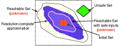
Figure 1: Probabilistic vs resolution completeness

To analyze the completeness properties of search based motion planning algorithms used in robotics, the notion of resolution completeness has been proposed in [18, 19]. A resolution-complete algorithm, is guaranteed to find a solution (if one exists), in finite time, provided that, the resolution of discretization in input space, and state space, is high enough. In [20, 21], we introduced a similar notion for disproving safety of continuous and hybrid systems over infinite time horizon, and, proposed resolution-complete deterministic algorithms applicable to linear time invariant systems (abbreviated as LTI systems). The algorithms work by incrementally building trajectories in state space at increasing levels of resolution, such that, either they fetch a legitimate counter example, or a guarantee that no such counter example exists at given level of resolution (and hence a conclusive answer to the unsafety problem), in finite time. In Fig. 1, at the right, we show an example where we end up with a non-zero volume under-approximation to reachable set (when no counter example was found), when using a sampling-based resolution-complete algorithm for safety falsification of a second order system with exogenous inputs [20].Very recently, an alternate notion of resolution completeness has also been proposed by Cheng and Kumar for continuous-time systems for the case of finite horizon in [22].

1.3 Contributions of the paper and relation to other approaches

In this paper, we propose two new resolution-complete algorithms that use incremental grid-based sampling methods (similar to those proposed in [23]) with good coverage properties for exploring the state space. The first algorithm uses breadth-first-search based scheme with branch and bound strategy to explore the state space for counter examples to given safety specification, at increasing levels of resolution of the input. This algorithm can be applied to discrete-time LTI hybrid systems. Simulation results indicate that this algorithm, is an improvement over the one proposed by us in [21] which is based on depth-first-search based scheme with branch and bound strategy. The second algorithm proposed in this paper can be used to falsify safety of discrete-time LTI continuous systems more efficiently, when the initial set is the equilibrium point. The reachable set for such initial conditions is a convex set. The proposed algorithm uses this fact to explore the state space more efficiently. Since both the algorithms are resolution-complete, they consider the safety falsification problem over infinite time horizon, with guarantees of finite-time termination of the search procedure and a conclusive answer at termination.

An important feature that distinguishes our approach from alternate approaches recently proposed by others (e.g. [24]) for addressing safety over infinite time horizon, is that the requirements on discretization of state space in our case do not depend on time length of trajectories. This is an important advantage by itself, and also helps the algorithms in avoiding the so called wrapping effect [25]. This means that, in case no counter example is found, then the quality of the approximation constructed as a proof for safety of the system is not affected by time horizon. We also do not discretize the space of inputs to obtain completeness guarantees (unlike the approaches presented in [22, 24]).

The paper is organized as follows. We introduce the framework for describing hybrid systems and reachable sets in Section 2 together with a formal definition of the notion of resolution completeness for safety falsification. In Section 3, we explain the main idea used in the proposed algorithms for resolution completeness. Conditions for resolution completeness of the proposed algorithms are discussed in Section 4. In Section 5, we explain the sampling method used by us in the algorithms and in Section 6, we present the algorithms, together with the proof of their completeness. Simulation results are discussed in Section 7, and the paper is concluded in Section 8.

2 Preliminaries

In this section, we introduce notation for describing hybrid systems and reachable sets and define the notion of resolution completeness.

Definition 1 (Hybrid System).

We define a discrete-time LTI hybrid system $H$ as a tuple, $H=(\mathcal{Q},\mathcal{X},\mathcal{U},U,\Phi,\Delta,\mathcal{I},\mathcal{S},\mathcal{T}),$ where:

• $\mathcal{Q}$ is the discrete state space.

• $\mathcal{X}\subseteq\mathbb{R}^{n}$ is the continuous state space.

• $\mathcal{U}$ is the family of allowed control functions equipped with a well defined metric. Each control function $u\in\mathcal{U}$ is a function $u:[0,t_{f}]\rightarrow U$, where $t_{f}\in\mathbb{N}$ is the terminal time of the trajectory. The convex set $U\subset\mathbb{R}^{m}$ is the input space. For simplicity, we assume $U$ to be a unit hypercube.

• $\Phi:\mathcal{Q}\times\mathcal{X}\times\mathcal{U}\rightarrow\mathcal{X}$ is a function describing the evolution of the system on continuous space, governed by a difference equation of the form $x(i+1)=\Phi(x,q,u)=A_{q}x(i)+B_{q}u(i),i\in\mathbb{N}$, and $A_{q},B_{q}$ are real matrices of size $n\times n,n\times m$ respectively.

• $\Delta\subset(\mathcal{Q}\times\mathcal{X})\times(\mathcal{Q}\times\mathcal{X})$, a relation describing discrete transitions in the hybrid states. Discrete transitions can occur on location-specific subsets $\mathcal{G}(q,q^{\prime})\subseteq\mathcal{X}$, called guards, and result in jump relations of the form $(q,x)\mapsto(q^{\prime},x)$.

• $\mathcal{I},\mathcal{S},\mathcal{T}\subseteq\mathcal{Q}\times\mathcal{X}$ are, respectively, the invariant set, the initial set, and the unsafe set.

The semantics of our model are defined as follows. When the discrete state is in location $q$, the continuous state evolves according to the difference equation $x(i+1)=A_{q}x(i)+B_{q}u(i),i\in\mathbb{N}$, for some value of the input $u(i)\in U$, with $(q(0),x(0))\in\mathcal{S}$. In addition, whenever $x(i)\in\mathcal{G}(q(i),q^{\prime})$, for some $q^{\prime}$, the system has the option to perform one of the discrete transitions modeled by the relation $\Delta$, and be instantaneously reset to the new discrete state $q^{\prime}$, while the continuous state remains the same as before the discrete transition. The system is required to respect the invariants by staying within $\mathcal{I}$ at all times. For the cases when the discrete state space is just a single location, we drop the discrete state $q$ from the notation. $\Omega=\{\bar{q},\bar{q}:[0,t_{f}]\rightarrow Q\}$ denotes the set of trajectories on the discrete space. Trajectories of the system starting from $z\in\mathcal{Q}\times\mathcal{X}$ and using $u\in\mathcal{U}$, under the discrete evolution $\bar{q}$, are denoted by $\Psi(z,u,\bar{q})\subset\mathcal{Q}\times\mathcal{X}$. A point on the trajectory $\Psi(z,u,\bar{q})$, reached at time $i\leq t_{f}$, is denoted by $\psi(z,u,\bar{q},i)\in\mathcal{Q}\times\mathcal{X}$. We will denote by $A^{\circ}$ the interior of a set $A$.

Definition 2 (Reachable Set).

The reachable set $\mathcal{R}(\mathcal{U})$ for a system $H$ denotes the set of states that can be reached in the future. It is defined as

$$\mathcal{R}(\mathcal{U})=\bigcup_{z\in\mathcal{S},\;u\in\mathcal{U},\;\bar{q}\in\Omega}\Psi(z,u,\bar{q}).$$

We now formalize the notion of resolution completeness of an algorithm for safety falsification of a discrete-time LTI system with exogenous inputs.

Definition 3 (Resolution completeness).

A given algorithm is resolution-complete for safety falsification of a system $H$, if there exists a sequence of family of control functions, $\{\mathcal{U}_{j}\}_{j=1}^{\infty}$, satisfying $\mathcal{U}_{j}\subset\mathcal{U}_{j+1},\forall j$, and $\lim_{j\to\infty}\mathcal{U}_{j}=\mathcal{U}$ (in the sense of a given metric), such that, for any given $j\geq 1$, the algorithm terminates in finite time, producing, either a counter example $\psi(z_{0},u,\bar{q},t)$, using a control function $u\in\mathcal{U},z_{0}\in\mathcal{S},\bar{q}\in\Omega,t\geq 0$, satisfying, $\psi(z_{0},u,\bar{q},t)\in\mathcal{T}$, or a guarantee that, $\mathcal{R}^{\circ}(\mathcal{U}_{j})\cap\mathcal{T}=\emptyset$.

3 Basic Idea

One way to achieve completeness is to construct an approximation $\mathcal{R}_{j}$ (while searching for a counter example) that satisfies the set inclusion $\mathcal{R}^{\circ}(\mathcal{U}_{j})\subseteq\mathcal{R}_{j}\subseteq\mathcal{R}(\mathcal{U})$ (shown in Fig. 3(a)), thus guaranteeing feasibility of counter examples and safety with respect to control functions belonging to $\mathcal{U}_{j}$. The algorithms that we propose in this paper use this idea. To construct $\mathcal{R}_{j}$, the algorithms discretize the state-space using multi-resolution grids. For a discrete location $q\in\mathcal{Q}$, $G(q)$ denotes the multi-resolution grid for location $q$ that over-approximates $\mathcal{R}\cap\mathcal{I}(q,\cdot)$. The algorithms keep a record of the portion of $G(q)$ that is found to be reachable (denoted as $G_{f}(q)$), either a priori or during an execution of the algorithm. $G_{u}(q)$ denotes the rest of $G(q)$, i.e. $G_{u}(q)=G(q)\setminus G_{f}(q)$. The algorithms progressively sample regions of $G_{u}(q)$ (called cells) at increasing levels of resolution and try to construct trajectories that end in the sampled cell starting from somewhere in $G_{f}(q)$. The conditions for state-space discretization derived in Section 4 guarantee that finding one feasible point $\psi(z_{0},u,\bar{q},t)$ in a cell $\xi(\varepsilon_{j}(q))$ of size $\varepsilon_{j}(q)$, with $z_{0}\in G_{f}(q),u\in\mathcal{U}_{j},\bar{q}\in\Omega$, is enough to claim that $\xi\subset\mathcal{R}(\mathcal{U})$.

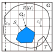
(a) Initialization step

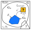
(b) Exploration step

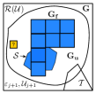
(c) Refinement step

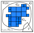
(d) Termination step

Figure 2: Execution of a resolution-complete algorithm for $\operatorname{card}{(\mathcal{Q})}=1$

In Fig. 2, we show an execution of such a resolution-complete safety falsification algorithm (starting at resolution $j$ and stopping at $j+1$) for the case when $\operatorname{card}{\mathcal{Q}}=1$.

We would like to remark here that, if we can find conditions that ensure the set inclusion, $\mathcal{R}^{\circ}(\mathcal{U}_{j})\subseteq\mathcal{R}_{j}\subseteq\mathcal{R}(\mathcal{U})$ for nonlinear systems, then similar algorithms can be used for resolution complete safety falsification of non linear systems as well.

4 Conditions for Resolution-Complete Safety Falsification

In this section, we derive necessary conditions for resolution-complete safety falsification of discrete-time LTI hybrid systems. For all the discussion that follows, $\lVert\cdot\rVert$ denotes the infinity norm. The set of control functions is, $\mathcal{U}=\{u(\cdot):\lVert u(i)\rVert\leq 1,\;\forall i\in\mathbb{N},i\leq t_{f}\}$. $\mathcal{C}_{q}=[B_{q}\;A_{q}B_{q}\ldots A_{q}^{n-1}B_{q}]$ denotes the controllability matrix of the system in location $q\in\mathcal{Q}$.

4.1 Control functions for resolution completeness

For resolution completeness, we need a sequence of control functions $\{\mathcal{U}_{j}\}_{j=1}^{\infty}$ such that $\mathcal{U}_{j}\subset\mathcal{U}_{j+1},\forall j\in\mathbb{N}$ and $\lim_{j\to\infty}\mathcal{U}_{j}=\mathcal{U}$ in some metric defined on the space of control functions. We consider sequence of families of piece-wise constant control functions for our algorithm.

Proposition 1.

For given family of control functions $\mathcal{U}$, the sequence of family of control functions $\{\mathcal{U}_{j}\}_{j=1}^{\infty}$, $\mathcal{U}_{j}=\{u(\cdot):\lVert u(i)\rVert\leq l_{j},\;\forall i\in\mathbb{N},i\leq t_{f},t_{f}\in\mathbb{N}\}$, with $\{l_{j}\}$ a strictly non decreasing sequence of real numbers and $\lim_{j\to\infty}l_{j}=1$ satisfies $\mathcal{U}_{j}\subset\mathcal{U}_{j+1},\forall j$ and $\lim_{j\to\infty}\mathcal{U}_{j}=\mathcal{U}$ in $L_{\infty}$ norm.

Proof.

The proposition is proved by stated requirements on $\{l_{j}\}$. $\blacksquare$

4.2 Assumptions

Assumption 1.

For each discrete location $q\in\mathcal{Q}$, the system $H$ is stable at the origin, $\operatorname{rank}{(B_{q})}=m$, and, $\operatorname{rank}{(\mathcal{C}_{q})}=n$.

Stability (along with Assumption 2) guarantees that $G(q)$ has a finite volume. $\operatorname{rank}{(B_{q})}=m$ and $\operatorname{rank}{(\mathcal{C}_{q})}=n$ is needed to be able to use Propositions 2, 3.

Assumption 2.

For each discrete location $q\in\mathcal{Q}$, $\mathcal{S}(q,\cdot),\mathcal{G}(q,\cdot)$ are specified as convex polytopes and $\mathcal{I}(q,\cdot),\mathcal{T}(q,\cdot)$ are specified as a convex polyhedra.

At each step, the algorithms incrementally build the trajectories and check for unsafety and discrete mode switches by solving linear programs. Hence we need the sets $\mathcal{S}(q\cdot),\mathcal{I}(q,\cdot),\mathcal{G}(q,\cdot),\mathcal{T}(q,\cdot)$ to be convex polyhedra. Boundedness of $\mathcal{S}(q,\cdot),\mathcal{G}(q,\cdot)$ is used to prove finite time termination of the algorithms.

We now consider continuous dynamics in a given discrete location $q\in\mathcal{Q}$, and derive sufficient conditions for discretization of cells in $G(q)$.

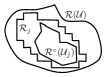
(a) Basic idea

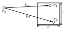
(b) One-step reachability

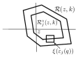
(c) k-step reachability

Figure 3: Set inclusions for resolution completeness

4.3 Sufficient conditions for state space discretization

We first state an important proposition that guarantees that the set of points $\psi(z,u,\bar{q},k)$, that can be searched by the algorithms for feasibility, starting from $z$, with $u\in\mathcal{U}_{j}$ (as in Proposition 1) in $k\in\mathbb{N}$ steps has a non zero volume. This follows from the assumption that $\operatorname{rank}{(B_{q})}=m$, and, $\operatorname{rank}{(\mathcal{C}_{q})}=n$ in each discrete location $q\in\mathcal{Q}$.

Proposition 2.

For a given system $H$ satisfying Assumption 1, and for a given location $q\in\mathcal{Q}$, the set of points reachable by using a control function $u\in\mathcal{U}_{j}$ (as in Proposition 1) over $k$ steps has a non empty interior if $\lceil n/m\rceil\leq k\leq n$ for any $j\geq 1$, where $n$ is the dimension of the continuous state space and $m$ is the dimension of input space.

Proof.

Let $k$ be chosen such that $\lceil n/m\rceil\leq k\leq n$. The continuous dynamics of the system are $x(i+1)=A_{q}x(i)+B_{q}u$, where $u\in\mathcal{U}_{j}$. Applying this over k steps, we get $x(k+i)=A_{q}^{k}x(i)+[B_{q}\;A_{q}B_{q}\ldots A_{q}^{k-1}B_{q}]\tilde{u}$, where $\tilde{u}\in\mathbb{R}^{km}$ is the augmented input over $k$ steps. Let $v=[B_{q}\;A_{q}B_{q}\ldots A_{q}^{k-1}B_{q}]\tilde{u}$. Then the dynamics can be written as $x(k+i)=A_{q}^{k}x(i)+v,v\in\mathbb{R}^{n}$. Since $\operatorname{rank}{(\mathcal{C}_{q})}=n$, $\operatorname{rank}{[B_{q}\;A_{q}B_{q}\ldots A_{q}^{k-1}B_{q}]}=n$. Hence the set of points reachable in $k$ steps is guaranteed to have a non empty interior. $\blacksquare$

We now derive a conservative upper bound on the discretization of $G(q)$, so that for a cell $\xi$, if $\xi\cap\mathcal{R}^{\circ}(\mathcal{U}_{j})\cap\mathcal{I}(q,\cdot)\neq\emptyset$ then $\xi\subset\mathcal{R}(\mathcal{U})\cap\mathcal{I}(q,\cdot)$. To do so, we first prove the result for a simpler case in Lemma 1, and then prove the main result in Propositon 3.

Lemma 1.

Consider a continuous system $H$, with $x(i+1)=Ax(i)+v$ with, $x$, $v\in\mathbb{R}^{n}$. For a given $x_{1}$, and an $\alpha_{1}>0$, with $x_{1}=Ax_{0}+v_{1},x_{0},v_{1}\in\mathbb{R}^{n},and,\lVert v_{1}\rVert\leq\alpha_{1}$, the following holds true: For any $x_{2}\in\mathbb{R}^{n}$, and a given $\alpha_{2}>\alpha_{1}$, if $\lVert x_{1}-x_{2}\rVert\leq\varepsilon$, and $\varepsilon\leq\alpha_{2}-\alpha_{1}$, then $\exists v_{2}\in\mathbb{R}^{n}$, such that, $x_{2}=Ax_{0}+v_{2}$, with, $\lVert v_{2}\rVert\leq\alpha_{2}$.

Proof.

Please refer to Fig. 3(b). $v_{2}=v_{1}+x_{2}-x_{1}$ proves the result. $\blacksquare$

Proposition 3.

Consider a system $H$ satisfying Assumption 1, with sequence of families of control functions $\{\mathcal{U}_{j}\}_{j=1}^{\infty}$, as in Proposition 2. Let $j\in\mathbb{N}$ and $q\in\mathcal{Q}$ be fixed. Then, if the cell size $\varepsilon_{j}(q)$ for a cell $\xi\in G(q)$ satisfies the bound, $\varepsilon_{j}(q)\leq(1-l_{j})/\lVert{\Gamma}^{+}_{q}\rVert$, where ${\Gamma_{q}}=[B_{q}\;A_{q}B_{q}\ldots A_{q}^{k-1}B_{q}]$ and ${\Gamma_{q}}^{+}$ is the pseudo inverse, then $\xi\cap\mathcal{R}^{\circ}(\mathcal{U}_{j})\cap\mathcal{I}(q,\cdot)\neq\emptyset\Rightarrow\xi\subset\mathcal{R}(\mathcal{U})\cap\mathcal{I}(q,\cdot)$.

Proof.

The dynamics of the system over $k$ steps can be written as $x(k+i)=A_{q}^{k}x(i)+v$, with $v=\Gamma_{q}\tilde{u}$. ${\Gamma_{q}}=[B_{q}\;A_{q}B_{q}\ldots A_{q}^{k-1}B_{q}]$ and $\tilde{u}\in\mathbb{R}^{km},\lVert\tilde{u}\rVert\leq l$ is the augmented input over $k$ steps. This implies that $\tilde{u}=\Gamma_{q}^{+}v$, where $\Gamma_{q}^{+}$ is the pseudo inverse of $\Gamma_{q}$. Finding the tightest bounds on $v$ is hard. However a conservative bound on $v$ is $\lVert v\rVert\leq l/\Gamma^{+}$. Now, let $v_{1}=\Gamma_{q}\tilde{u}_{1}$ and $v_{2}=\Gamma_{q}\tilde{u}_{2}$ with $\tilde{u}_{1},\tilde{u}_{2}\in\mathbb{R}^{km}$ and $\lVert\tilde{u}_{1}\rVert\leq l_{j}$ and $\lVert\tilde{u}_{2}\rVert\leq 1$. Let $\mathcal{R}(z,k)$ denote set of points reachable by the system by using $u\in\mathcal{U}$ with $t_{f}=k$, and $\mathcal{R}_{j}^{\circ}(z,k)$ the interior of the set of points reachable by the system by using $u^{\prime}\in\mathcal{U}_{j}$ with $t_{f}=k$, under continuous evolution, starting from $z$. This is shown in Fig. 3(c). The result of Lemma 1 implies that for $\varepsilon_{q}\leq(1-l_{j})/\Gamma_{q}^{+}$, $\xi\cap\mathcal{R}_{j}^{\circ}(z,k)\neq\emptyset\Rightarrow\xi\subset\mathcal{R}(z,k)$. This proves that $\xi\cap\mathcal{R}^{\circ}(\mathcal{U}_{j})\cap\mathcal{I}(q,\cdot)\neq\emptyset\Rightarrow\xi\subset\mathcal{R}(\mathcal{U})\cap\mathcal{I}(q,\cdot)$. $\blacksquare$

5 Incremental Grid Sampling Methods

As we discussed in Section 3, for each location $q\in\mathcal{Q}$, we use a multi-resolution grid. Assume for this section that, $\operatorname{card}{(\mathcal{Q})}=1$, and that, $G$ is a $n$-dimensional unit cube, whose origin is the origin of coordinate axis. Using an iteratively refined multi-resolution grid ensures that for a given $j$, $G_{u}$ with resolution $\varepsilon_{j}$ does not have to be built from scratch. For our work, we will use multi resolution classical grids. A multi-resolution classical grid at resolution level $r$ has $2^{rn}$ points. Moreover, it contains all the points of all the resolution levels $r^{\prime}<r$. Every grid point $P_{i}$, in a multi resolution classical grid at resolution level $r$, can be written as $P_{i}=\{\frac{a_{1}}{2^{r}},\ldots,\frac{a_{n}}{2^{r}}\}$ with $0\leq a_{1},\ldots,a_{n}\leq 2^{r}-1$, $a_{1},\ldots,a_{n}\in\mathbb{N}$, with the corresponding grid region (that we call as cells) $\xi(r,i)=[\frac{a_{1},a_{1}+1}{2^{r}})\times\ldots[\frac{a_{n},a_{n}+1}{2^{r}})$. Here $i$ is the unique identifier for each cell $\xi$, and it denotes its order in the generated samples. For any resolution level $j$, the resolution level $j+1$ satisfies $\varepsilon_{j+1}=\varepsilon_{j}/2$. For any two cells $\xi_{1},\xi_{2}$, at resolution levels $r_{1},r_{2}$ respectively, with $r_{1}<r_{2}$, and, $\xi_{1}\cap\xi_{2}\neq\emptyset$, $\xi_{1}$ will be called as the parent of $\xi_{2}$ at resolution $r_{1}$, and, $\xi_{2}$ as a child of $\xi_{1}$ at resolution $r_{2}$.

Ideally, one would like to use an ordering of samples that minimizes the discrepancy to find a counter-example as soon as possible. But discrepancy-optimal orderings take exponential time to compute, and exponential space to be stored (in $n$; see  [23]). For our work, we use orderings that maximize the mutual distance between sampled grid points (see  [23]). The mutual distance of a set $\mathcal{K}$ is defined as $\rho_{m}(\mathcal{K})=\min_{x,y\in\mathcal{K}}\rho(x,y)$. These orderings can be represented by using generator matrices, that are binary matrices of size $n\times n$ and represent bijective linear transformation over $\mathbb{Z}_{2}$. Any sample with identifier $i$, at resolution $j$, can be generated by using the ordering recursively on the bit representation of $i$. This method can also be used to bias the search towards the unsafe set $\mathcal{T}$, by possibly changing the generator matrix. In Fig. 4, we show the samples for few resolution levels in 2 dimensions. As can be seen, cells whose identifiers are close to each other (e.g. Resolution $=2$ or $3$, $i=0,1$) are spaced quite far apart. This is in sharp contrast to the ordering that one would get by using a naive sampling scheme, like scanning for example.

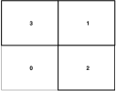
(a) Resolution$=1$

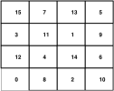
(b) Resolution$=2$

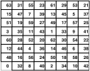
(c) Resolution$=3$

Figure 4: Ordering of samples based on mutual distance

6 Algorithms for Resolution-Complete Safety Falsification

In this section, we first explain the procedure for incremental construction of trajectories used by the algorithms. We then present the algorithms, and in Section 6.4, prove their resolution completeness.

6.1 Incremental construction of trajectories

As stated in Section 4.1, the algorithms use piece-wise constant control functions satisfying Proposition 2. As discussed in the proofs of Propositions 2, 3, for a given discrete state $q\in\mathcal{Q}$, the dynamics can be simulated by using $x(k)=A_{q}^{k}x_{0}+v$, where $x_{0}\in\mathcal{I}(q,\cdot)$, and, the set of feasible inputs is given by $v={\Gamma_{q}}\tilde{u}$, $\tilde{u}\in\mathbb{R}^{km}$, $\lVert\tilde{u}\rVert\leq\tilde{l}_{j}(q)=1-\varepsilon_{j}(q)\lVert{\Gamma_{q}}^{+}\rVert$. Note, that to be less conservative, we are making the input bound $\tilde{l}_{j}(q)$ dependent on $q\in\mathcal{Q}$ and the discretization $\varepsilon_{j}(q)$. Hence, the algorithms use the input bounds based on the space discretization and dynamics to incrementally build trajectories $k$ steps at a time, by formulating the $k$-step reachability problem as a linear program. To solve these linear programs more efficiently, we use ideas from [26] for multi parametric linear programming.

We use the following additional notation in the remaining of this section. $G=\cup_{q\in\mathcal{Q}}G(q)$ denotes the union of all location specific grids in the algorithm. $j_{0}$ represents the smallest $j$, such that $\tilde{l}_{j_{0}}(q)=1-\varepsilon_{j_{0}}(q)\lVert{\Gamma_{q}}^{+}\rVert>0,\forall q\in\mathcal{Q}$. For all $j>j_{0}$, and, $\forall q\in\mathcal{Q}$, $\tilde{l}_{j}(q)=1-\varepsilon_{j}(q)\lVert{\Gamma_{q}}^{+}\rVert$. $\varepsilon_{j}$ is a $Q$-dimensional vector with each element denoting value for a given location $q$. Since $\tilde{l}_{j}(q)$ can be different for each discrete location $q\in\mathcal{Q}$, at termination of the algorithms, completeness will be guaranteed with respect to $l_{j}=\min_{q\in\mathcal{Q}}\tilde{l}_{j}(q)$.

6.2 Breadth First Search with Branch and Bound

The proposed algorithm is shown in Fig. 6. We will refer to this algorithm as the BFS-BB Safety Falsification algorithm. A few iterations of the algorithm for a first order discrete-time LTI system with single discrete mode, are shown in Fig. 5 for a maximum resolution level of $j=3$.

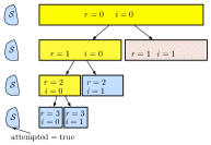
Exploration starting from $\mathcal{S}$

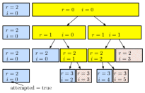
Exploration starting from $\xi(r=2,i=0)$

Figure 5: An execution of BFS-BB Safety Falsification algorithm

Cells marked in yellow are the ones that need to be explored further based on branch and bound strategy. Cells marked in red are conclusively not reachable from $\xi_{f}$ (where $\xi_{f}\in G_{f}$ is $\mathcal{S}$ at the left and $\xi(r=2,i=0)$ at the right). Cells marked in blue are the ones that are found to be reachable.

 BFS-BB Safety Falsification ($H$, $j_{\mathrm{max}}$, $G$)  

1  $\{\mathit{locations},\mathit{Found}\}\leftarrow\{\emptyset,\emptyset\}$

2  $\{j_{0},G_{f},\mathit{locations}\}\leftarrow$ init($H.\mathcal{S}$) //Initialization step

3  $j\leftarrow j_{0}$

4  while ($j\leq j_{\mathrm{max}}\wedge\neg\mathit{Found}$) do

5     for all ($q\in\mathit{locations}$) do

6        update_explorer($q$,$j$) //Update simulation parameters for current $j,q$

7        for all ($\xi_{\mathrm{f}}\in G_{f}(q)\wedge\neg\mathit{Found}$) do

8           for all ($r\in\{1,2,\ldots,j\}$) do

9              for all ($i\in\{0,\ldots,2^{rn}-1\}$) do

10                 if ($\mathit{Found}$) then

11                    return $(G_{f},\mathit{Found},\varepsilon_{j})$ //Terminate if unsafe

12                 $\xi_{t}\leftarrow$generate_sample($i,r,q$) //Sample generation

13                 if (check_feasible($\xi_{t}$)) then

14                    $\mathit{success}\leftarrow$ expand($\xi_{f},\xi_{t}$) //Expansion step

15                    if ($\mathit{success}$) then

16                       add_node($\xi_{f},\xi_{t}$) //Update of $G_{f}(q)$

17                       $\mathit{Found}\leftarrow$ check_unsafety($\xi_{t}$) //Check for unsafety

18           $\xi_{f}.\mathit{attempted}\leftarrow\mathrm{true}$ //Mark as attempted

19        $\mathit{locations}$.erase($q$)

20     $j+1\leftarrow G$.refine(j) //Refinement step

21  return $(G_{f},\mathit{Found},\varepsilon_{j})$

 

Figure 6: BFS-BB Safety Falsification algorithm

Data structure: Each cell $\xi$ has its identifier $i$, resolution level $r$, and boolean variables $\mathit{attempted,filled}$. $\mathit{attempted}$ is true, if, $\xi\in G_{f}(q)$ has been attempted for expansion (and the cell is called attempted). The variable $\mathit{filled}$ is true (and the cell is called as filled) if, the cell $\xi$ has size $\epsilon_{j}(q)$ (for some $j$) and is found to be reachable using $\tilde{l}_{j}(q)$, or, all its children at resolution $j+1$ are filled. $G_{f}$ is implemented as a hash map to enable quick look up for existing cells in $G_{f}$.

Initialization step: In the first step, the algorithm computes the first feasible resolution level $j_{0}$ and initializes $G_{f}(q)$ $\forall q\in\mathcal{Q}$. Next all $q\in\mathcal{Q}$ are added to $\mathit{locations}$ for which $G_{f}\neq\emptyset$. This happens in init($H.\mathcal{S}$) function in the algorithm.

Exploration step: The grid is searched for reachable cells with current bounds on input in a recursive Breadth-First-Search (BFS) fashion along with Branch and Bound (BB) strategy in the algorithm for each location $q\in\mathit{locations}$ (after updating the simulation parameters used by the algorithm for location $q$ in update_explorer($q,j$) function in the algorithm). First, a filled cell $\xi_{f}$ is chosen in $G_{f}(q)$. Next, for all depths $r\in\{1,\ldots,j\}$ samples $\xi_{t}$ are generated in generate_sample($i,r,q$) function (after checking if $\mathit{Found}=\emptyset$). The function check_feasible($\xi_{t}$) checks feasibility of $\xi_{t}$ based on branch and bound condition from coarse resolution levels, and the fact that its parent might have been marked as filled already at some coarser resolution level $r^{\prime}<r$. The expand($\xi_{f},\xi_{t}$) function attempts to solve the $k$-step reachability problem as discussed in Section 6.1. If it is successful then the add($\xi_{f},\xi_{t}$) function adds $\xi_{f}$ to $G_{f}(q)$.

Unsafety check: Each newly added cell $\xi_{t}$ in add($\xi_{f},\xi_{t}$) step is checked for intersection with the unsafe set $\mathcal{T}$, if, it is filled, in check_unsafety($\xi_{t}$) function.

Discrete transition step: For a given location $q$, each cell $\xi\in G(q)$ that is found to be reachable from $G_{f}(q)$ is checked for all the outgoing discrete transitions from $q$. If a guard $\mathcal{G}(q,q^{\prime})$ is found to be enabled, then $\mathcal{G}(q,q^{\prime})\cap\xi$ is added as a filled cell to $G_{f}(q^{\prime})$ using the function add($\xi,\mathcal{G}(q,q^{\prime})\cap\xi$) and $q^{\prime}$ is added to $\mathit{locations}$. This happens internally in add($\xi_{f},\xi_{t}$) function.

Refinement step: When all the cells $\xi_{f}\in G_{f}(q)$ have been explored for expansion $\forall q\in\mathcal{Q}$, and $\mathit{locations}=\emptyset$, then the grid resolution is changed using the relation $\varepsilon_{j+1}(q)=$$\varepsilon_{j}(q)/2$, and the input bounds are changed from $\tilde{l}_{j}(q)$ to $\tilde{l}_{j+1}(q)$. For all the cells $\xi\in G_{f}(q)$, and, $\forall q\in\mathcal{Q}$, the variable $\mathit{attempted}$ is reset to false. This happens in the $G$.refine(j) function in the algorithm.

Termination criteria: To have a finite termination time, the refinement procedure is allowed only till $j\leq j_{\mathrm{max}}$, and, no counter example has been found.

6.3 Resolution-complete Co-RRT

In this section, we discuss a modified version of the Co-RRT algorithm proposed by us in [13] for continuous systems that is resolution-complete. This algorithm can be used for analyzing safety of a continuous system when it starts from equilibrium under the effect of exogenous inputs. We first state an important lemma regarding reachability of points that are convex combinations of two reachable points.

Proposition 4.

For an origin-stable, continuous system $H$, if $\mathcal{S}=\{0\}$, then for any two reachable points $\psi_{1}(0,u_{1},k_{1}),\psi_{2}(0,u_{2},k_{2}),u_{1},u_{2}\in\mathcal{U},k_{1},k_{2}\in\mathbb{N},k_{2}\geq k_{1}$, the convex combination $\psi_{\lambda}=\lambda\psi_{1}+(1-\lambda)\psi_{2},\lambda\in[0,1]$ is also reachable in $k_{2}$ time steps.

Proof.

$\psi_{1}(0,u_{1},k_{1})=[BAB\ldots A^{k_{1}-1}B]u_{1}$, $\psi_{2}(0,u_{1},k_{2})=[BAB\ldots A^{k_{2}-1}B]$$u_{2}$. $u_{1},u_{2}\in\mathbb{R}^{k_{1}m},\mathbb{R}^{k_{2}m}$ respectively. Let $\tilde{B}_{k}=[BAB\ldots A^{k-1}B]$, and, $\theta_{c}\in\mathbb{R}^{c}$, denote the zero vector. This implies that $\psi_{\lambda}=\lambda\tilde{B}_{k_{2}}[u_{1}^{\prime}\theta_{m(k_{2}-k_{1})}^{\prime}]^{\prime}+(1-\lambda)\tilde{B}_{k_{2}}u_{2}$. Since $U$ is convex, $u_{\lambda}=\lambda[u_{1}^{\prime}\theta_{m(k_{2}-k_{1})}^{\prime}]^{\prime}+(1-\lambda),u_{2}\in\mathcal{U}$. $\blacksquare$

Corollary 1.

$\mathcal{R}(\mathcal{U})$ is a convex set for a system $H$ (as in Proposition 4).

The proposed algorithm, called as the Co-RC Safety Falsification algorithm, is shown in Fig. 8. In Fig. 7, we show a few iterations of the algorithm for a second order system.

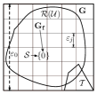
(a) Initialization step

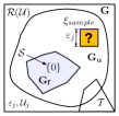
(b) Exploration step

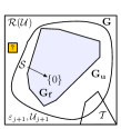
(c) Refinement step

(d) Termination step

Figure 7: An execution of Co-RC Safety Falsification algorithm

 Co-RC Safety Falsification ($H$, $j_{\mathrm{max}}$, $G$)  

1  $\mathit{Found}\leftarrow\emptyset$

2  $\{j_{0},G_{f}.\mathrm{Hull}\}\leftarrow G$.init($H.\mathcal{S}$) //Initialization step

3  $j\leftarrow j_{0}$,$\mathit{change}\leftarrow\mathrm{false}$

4  while ($j\leq j_{\mathrm{max}}\wedge\neg\mathit{Found}$) do

5     update_explorer($j$) //Update the simulation parameters for current j

6     repeat

7        $\mathit{change}\leftarrow\mathrm{false}$

8        for all ($r\in\{1,\ldots,j\}$) do

9           for all ($i\in\{0,\ldots,2^{rn}-1\}$) do

10              if ($\mathit{Found}$) then

11                 return $(G_{f},\mathit{Found},\varepsilon_{j})$ //Terminate if unsafe

12              $\xi_{t}\leftarrow$generate_sample($i,r$) //Sample generation

13              if (check_feasible($\xi_{t}$)) then

14                 $\mathit{success}\leftarrow$ expand($G_{f}.\mathrm{Hull},\xi_{t}$) //Expansion step

15                 if ($\mathit{success}$) then

16                    $\mathit{change}\leftarrow\mathrm{true}$

17                    $G_{f}.\mathrm{Hull}\leftarrow$ Co($G_{f}.\mathrm{Hull},\xi_{t}$) //Update the Hull

18                    $\mathit{Found}\leftarrow$ check_unsafety($G_{f}.\mathrm{Hull}$) // Unsafety check

19     until ($\neg\mathit{change}$)

20     $j+1\leftarrow G$.refine(j) //Refinement step

21  return $(G_{f},\mathit{Found},\varepsilon_{j})$

 

Figure 8: Co-RC Safety Falsification algorithm

Data structure: The data structure is the same as one in previous algorithm except that $G_{f}$ now contains a special node $G_{f}.\mathrm{Hull}$ that contains the information about the convex hull and which is used for actual expansion step, and unsafety checks.

Initialization step: In the first step, the algorithm computes the $j_{0}$, and, $G_{f}.\mathrm{Hull}$ is initialized to $\mathcal{S}$. This is done in init($H.\mathcal{S}$) function in the algorithm.

Exploration step: The sample generation and search strategy are similar to previous algorithm. The function check_feasible($\xi_{t}$) checks feasibility of $\xi_{t}$ based on the fact that $\xi_{t}$ may be contained inside $G_{f}.\mathrm{Hull}$, i.e, $\xi_{t}\subset G_{f}.\mathrm{Hull}$, or, its parent may not be reachable with the current $G_{f}$. In such a case, the function check_feasible($\xi_{t}$) returns false. If it returns true, then the expand($G_{f}.\mathrm{Hull},\xi_{t}$) function attempts to solve the $k$-step reachability problem as discussed in Section 6.1. If it is successful, then the Co($G_{f}.\mathrm{Hull},\xi_{t}$) function updates $G_{f}.\mathrm{Hull}$ in the function Co($G_{f}.\mathrm{Hull},\xi_{f}$). The operator Co updates $G_{f}.\mathrm{Hull}$ to the convex combination of $G_{f}.\mathrm{Hull}$ and vertices of the cell $\xi_{t}$.

Unsafety check: Each time a new cell is added to $G_{f}$, intersection of $G_{f}.\mathrm{Hull}$ and $\mathcal{T}$ is checked in the function check_unsafety($G_{f}.\mathrm{Hull}$).

Refinement step: When all the cells at a given resolution level $j$ have been explored (possibly repeatedly) for reachability from $G_{f}.\mathrm{Hull}$ and no new cell can be reached, the grid resolution is increased according to the relation $\varepsilon_{j+1}=\max(\varepsilon_{j}/2,\varepsilon_{min})$, and the input bounds are changed from $l_{j}$ to $l_{j+1}$.This happens in the $G$.refine(j) function in the algorithm.

Termination criteria: To have a finite termination time, the refinement procedure is allowed only till $j\leq j_{\mathrm{max}}$, and, no counter example has been found.

We next discuss the resolution completeness of the proposed algorithms.

6.4 Resolution completeness

We first prove two important lemmas required to prove the main result in Theorem 1. The first lemma proves that for a given maximum resolution level $j\geq j_{0}$, the algorithms terminate in finite time, and the second lemma proves the required set inclusion for resolution completeness.

Lemma 2.

Consider a LTI discrete-time hybrid system $H$ and a given $j_{\mathrm{max}}\geq j_{0}$. Then the Safety Falsification algorithms terminate in finite time.

Proof.

Consider the CoRC Safety Falsification algorithm first. The algorithm starts with the value $\varepsilon_{j_{0}}$ initially. If at any stage a counter example is found, finite time termination is trivially guaranteed. Otherwise, note that by Assumptions 1, 2, G is guaranteed to have a finite volume. Since there is a given bound $j_{\max}$ on the resolution, it is guaranteed that the algorithm will be able to refine the resolution only a finite number of times. The sum of the number of cells over all the possible refinements of the grid $G$ is given by $N_{\mathrm{cells}}=\frac{2^{n\lceil\varepsilon_{0}/\varepsilon_{j_{\mathrm{max}}}\rceil}-1}{2^{n}-1}$. Hence in the worst case, the algorithm terminates within $N_{\mathrm{cells}}^{2}$ iterations. Now consider the BFS-BB Safety Falsification algorithm. We have $\lvert\mathcal{Q}\rvert$ locations. For each location $q$, let $N_{\mathrm{cells}(q)}$ be the total number of cells over all possible refinements. The number of guards can be no more than $\lvert\mathcal{Q}\rvert^{2}$. Hence, in the worst case, the algorithm terminates within $\lvert\mathcal{Q}\rvert^{2}\max_{q\in\mathcal{Q}}N_{\mathrm{cells}(q)}^{2}$ iterations.

$\blacksquare$

Lemma 3.

Consider a LTI discrete-time hybrid system $H$ and a given $j_{\mathrm{max}}\geq j_{0}$. Then the Safety Falsification algorithms find a feasible counter example or else generate an approximation $\mathcal{R}_{j_{\mathrm{max}}}$ such that $\mathcal{R}^{\circ}(\mathcal{U}_{j_{\mathrm{max}}})\subseteq\mathcal{R}_{j_{\mathrm{max}}}\subseteq\mathcal{R}(\mathcal{U})$.

Proof.

For a given $j_{\mathrm{max}}$, $l_{j_{\mathrm{max}}}$ is fixed. The set inclusion $\mathcal{R}_{j_{\mathrm{max}}}\subseteq\mathcal{R}(\mathcal{U})$ follows from the discussion in Section 3, and Proposition 2,  3. This guarantees feasibility of the counter examples found by the algorithms. For a location $q\in\mathcal{Q}$, if a point is found reachable by the algorithms in a cell $\xi$, then the algorithms mark that cell as reachable based on the relaxation of input bounds from $l_{j}(q)$ to $1$, where $j_{0}\leq j\leq j_{\mathrm{max}}$. As a result we are guaranteed that when the algorithms terminate, the set inclusion $\mathcal{R}^{\circ}(\mathcal{U}_{j_{\mathrm{max}}})\subseteq\mathcal{R}_{j_{\mathrm{max}}}$ also holds true. Taking convex combinations of reachable cells in the CoRC Safety Falsification algorithm does not violate this inclusion. $\blacksquare$

Theorem 1.

Consider a LTI discrete-time hybrid system $H$ as in Lemmas 2, 3. Then the Safety Falsification algorithms are resolution complete for the system $H$.

Proof.

Let $j_{\mathrm{max}}\geq j_{0}$ be given. Proposition 1 guarantees the existence of required sequence of family of control functions. From Lemma 3 we know that if a counter example is found it is feasible. If no counter example is found, then it implies that there doesn’t exist one (using the class of control functions $\mathcal{U}_{j_{\mathrm{max}}}$), from the set inclusion proved in Lemma 3. Moreover,, Lemma 2 guarantees that the algorithms will terminate in a finite time. $\blacksquare$

7 Simulation Results

In this section, we present the simulations results obtained on different discrete time systems.The implementation has been carried out in C++ on a Pentium 4, 2.4 GHz machine, with 512 MB of RAM.We will examine the performance of algorithms presented in Section 6.2 (called as BFS-BB), Section 6.3 (called as CoRC) and the one presented in [21], which is based on Depth-First-Search with Branch and Bound strategy (called as DFS-BB).

7.1 Safety falsification of a discrete-time fifth-order system

The example presented in this section is mainly intended to investigate performance of different algorithms for problems in moderate dimensions. We consider a fifth-order system, with dynamics specified as: $x(i+1)=Ax(i)+Bu(i)$, $A=0.6065$ I, $B=3.935$ I. The initial set is $\mathcal{S}=\{0\}$. The simulation parameters are as follows: $\varepsilon_{0}=27.2,j_{\mathrm{max}}=4$. This corresponds to $\lVert u\rVert\leq 0.5679$. The unsafe set is a hypercube of size 0.90 and is given by $\mathcal{T}=x+[-0.45,0.45]^{5}$. We did 50 test runs each with an unsafe set randomly centered at $x$, where $x\in[-7,7]^{5}$ was chosen using a uniform distribution.

The performance results using different algorithms are shown in Fig. 9. The performance results indicate that when ever a counter example was found, all the algorithms terminated within 5 minutes. The BFS-BB algorithm falsifies safety sooner than other two algorithms. From the results, it is difficult to comment if CoRC performs better than DFS-BB or not. We have also done some profiling of the CoRC algorithm, and have found that almost 70% of the time is spent in removing the redundant vertices of the hull in the Co($G_{f}.\mathrm{Hull},\xi_{f}$) function. In our current implementation, we reconstruct the convex hull from scratch every time the Co($G_{f}.\mathrm{Hull},\xi_{f}$) function is called. We are working on using software libraries that support incremental construction of convex hulls.

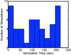
(a) Performance of DFS-BB

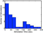
(b) Performance of BFS-BB

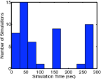
(c) Performance of CoRC

Figure 9: Performance comparison of different algorithms for fifth-order system

7.2 Safety falsification of a discrete-time second-order hybrid system

We now consider a second-order hybrid system with two discrete states. The example is interesting because of the fact that the guards and the invariants are all the same, and hence there is a potential problem of cycles. The dynamics are specified as $x(i+i)=A_{q}x(i)+B_{q}u(i),q\in\{1,2\}$, with, $A_{1}=[0.679\;0.404;-0.674\;0.140]$, $B_{1}=[0.440;-0.213]$, $A_{2}=[0.679\;-0.404;0.674\;0.140]$, $B_{2}=[0.3486;-0.1628]$. $\mathcal{I}(1,\cdot)=\mathcal{I}(2,\cdot)=\mathcal{G}(1,2)=\mathcal{G}(2,1)=[-2,2]^{2}$. The initial set is $\mathcal{S}=0\times[-0.1248,0.1248]^{2}$. The simulation parameters are $\varepsilon_{0}=4,j_{\mathrm{max}}=7$. Corresponding to this $\lVert u\rVert\leq 0.792$ for $q=0$, and $\lVert u\rVert\leq 0.869$ for $q=1$. Hence, for the case when no counter example is found, completeness will be guaranteed for $\lVert u\rVert\leq 0.792$.

The simulations are run for two cases based on the size of the unsafe set. In Case I, the unsafe set is small which makes it more difficult to be found by the explorer. However, quite often the unsafe set is specified as a large set (e.g. a half space representing the separation between two cars or aircrafts). To evaluate the performance of the algorithm for such cases, we present test runs in Case II. We did 200 runs for both the cases.
Case I: Small unsafe sets: For this case, the unsafe set is given by: $\mathcal{T}=q_{r}\times\{x+[-0.1,0.1]^{2}\}$, where $x\in[-1.5,1.5]^{2}$, was chosen using a uniform distribution and $q_{r}\in\{0,1\}$.
Case II: Large unsafe sets: For this case, we chose the unsafe set as a randomly oriented half space, given by: $\mathcal{T}=q_{r}\times\{(x_{1},x_{2}):mx_{1}+ax_{2}\leq c\}$, where, $m\in[-3.73,3.73],c\in[-1.9,0]$,$q_{r}\in\{0,1\}$, and $a=-\operatorname{sgn}(c)$. $c,m$ are chosen from a uniform distribution such that $\mathcal{S}\cap\mathcal{T}=\emptyset$.

Fig. 10 and Fig. 11 show performance results for the two cases along with a run when a counter example was found. Both the DFS-BB and BFS-BB algorithms falsify safety sooner for Case II.The BFS-BB falsifies safety in less than 10 seconds for 68 cases, compared to 54 for DFS-BB in Case I, and 164 times compared to 149 times for Case II.

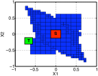
(a) Example for Case 1

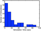
(b) Performance of DFS-BB

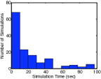
(c) Performance of BFS-BB

Figure 10: Safety falsification example and performance for Case I

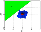
(a) Example for Case II

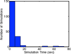
(b) Performance of DFS-BB

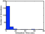
(c) Performance of BFS-BB

Figure 11: Safety falsification example and performance for Case II

8 Conclusions

In this paper, we have presented sampling-based resolution-complete algorithms for safety falsification of linear time invariant discrete-time systems over infinite time horizon. The algorithms attempt to generate a legitimate counter example by incrementally building feasible trajectories in the state space at increasing levels of resolution or provides a guarantee in a finite time that no such example exists, when the input is restricted to a certain class. As an additional result, when no counter example is found, the algorithms provide us with an arbitrarily good under approximation to the reachable set whose quality is independent of length of trajectories. Efforts are currently underway to develop more efficient algorithmsthat combine the nice features of both the depth-first-search and the breadth-first-search strategies to explore the state space.We are also investigating if its possible to develop similar algorithms for nonlinear systems.

9 Acknowledgements

We are grateful to S. LaValle, P. Cheng, S. Lindermann, and M. Branicky for stimulating discussion on the subject of this paper. We would also like to thank R. Majumdar for providing constructive suggestions on issues related to algorithmic complexity and improvements and F. Borrelli for providing useful suggestions on implementation of multi-parametric optimization in our work.We would also like to thank S. Lindermann for providing us with the code used to generate optimal orderings based on mutual distance, and R. Sanfelice for useful suggestions on the presentation of this paper. The research leading to this work was supported by the National Science Foundation (grants number 0715025 and 0325716).

References

- [1] Yonit Kesten, Amir Pnueli, Joseph Sifakis, and Sergio Yovine. Integration graphs: A class of decidable hybrid systems. In Hybrid Systems, pages 179–208. Springer-Verlag, 1993.
- [2] R. Alur, C. Courcoubetis, N. Halbwachs, T.A. Henzinger, P.H. Ho, X. Nicollin, A. Olivero, J. Sifakis, and S. Yovine. The algorithmic analysis of hybrid systems. Theoretical Computer Science, 138:3–34, 1995.
- [3] T.A. Henzinger and P. H. Ho. HyTech: the Cornell Hybrid Technology Tool. In P. J. Antsaklis, W. Kohn, A. Nerode, and S. Sastry, editors, Hybrid Systems II, volume 999 of Lecture Notes in Computer Science. Springer-Verilag, 1995.
- [4] R. Alur, T. Dang, and F. Ivanc̆ić. Reachability analysis of hybrid systems via predicate abstraction. In C. J. Tomlin and M. R. Greenstreet, editors, Hybrid Systems: Computation and Control, Lecture Notes in Computer Sciences, pages 35–48. Springer, 2002.
- [5] Stephen Prajna and Ali Jadbabaie. Safety verification of hybrid systems using barrier certificates. In Rajeev Alur and George J. Pappas, editors, Hybrid Systems: Computation and Control, volume 2993 of Lecture Notes in Computer Science, pages 477–492. Springer, 2004.
- [6] A. Chutinan and B. H. Krogh. Verification of polyhedral-invariant hybrid automata using polygonal flow pipe approximations. In Hybrid Systems: Computation and Control, volume 1569. Springer, 1999.
- [7] Eugene Asarin, Olivier Bournez, Thao Dang, and Oded Maler. The d/dt tool for verification of hybrid systems. In Proceedings of the Conference on Computer-Aided Verification, volume 2404 of Lecture Notes in Computer Science, pages 365–370. Springer, 2002.
- [8] A. B. Kurzhanski and P. Varaiya. Ellipsoidal techniques for reachability analysis. In Hybrid Systems: Control and Computation, volume 1790 of Lecture Notes in Computer Science. Springer-Verlag, 2000.
- [9] I. Mitchell and C. Tomlin. Level set methods for computation in hybrid systems. In Hybrid Systems: Computation and Control, volume 1790. Springer, 2000.
- [10] Antoine Girard. Reachability of uncertain linear systems using zonotopes. In Manfred Morari, Lothar Thiele, and Francesca Rossi, editors, Hybrid Systems: Computation and Control, volume 3414 of Lecture Notes in Computer Science, pages 291–305. Springer-Verilag, 2005.
- [11] Stefan Ratschan and Zhikun She. Safety verification of hybrid systems by constraint propagation-based abstraction refinement. ACM Trans. Embedded Comput. Syst., 6(1), 2007.
- [12] B. I. Silva, O. Stursberg, B. H. Krogh, and S. Engell. An assessment of the current status of algorithmic approaches to the verification of hybrid systems. In Proceedings of the 40th Annual Conference on Decision and Control, volume 3, pages 2867 – 2874, 2001.
- [13] Amit Bhatia and Emilio Frazzoli. Incremental search methods for reachability analysis of continuous and hybrid systems. In Rajeev Alur and George J. Pappas, editors, Hybrid Systems: Computation and Control, volume 2993 of Lecture Notes in Computer Science, pages 142–156. Springer, 2004.
- [14] C. Belta, J. M. Esposito, J. Kim, and R. V. Kumar. Computational techniques for analysis of genetic network dynamics. International Journal of Robotics Research, 24(2-3):219–235, 2005.
- [15] Alexandre Donzé and Oded Maler. Systematic simulation using sensitivity analysis. In Alberto Bemporad, Antonio Bicchi, and Giorgio C. Buttazzo, editors, Hybrid Systems: Control and Computation, volume 4416 of Lecture Notes in Computer Science, pages 174–189. Springer, 2007.
- [16] Tarik Nahhal and Thao Dang. Guided randomized simulation. In Alberto Bemporad, Antonio Bicchi, and Giorgio C. Buttazzo, editors, Hybrid Systems: Control and Computation, volume 4416 of Lecture Notes in Computer Science, pages 731–735. Springer, 2007.
- [17] S. M. LaValle and J. J. Kuffner. Rapidly-exploring random trees: Progress and prospects. In B. R. Donald, K. M. Lynch, and D. Rus, editors, Algorithmic and Computational Robotics: New Directions, pages 293–308. A.K. Peters, Wellesley, MA, 2001.
- [18] P. Cheng and S. M. LaValle. Resolution completeness for sampling-based motion planning with differential constraints. International Journal of Robotics Research, 2004. Submitted.
- [19] K. Goldberg. Completeness in robot motion planning. In Workshop on Algorithmic Foundations of Robotics, pages 419–429, 1994.
- [20] Amit Bhatia and Emilio Frazzoli. Resolution complete safety falsification of continuous time systems. In Conference on Decision and Control, 2006.
- [21] Amit Bhatia and Emilio Frazzoli. Sampling-based resolution-complete safety falsification of linear hybrid systems. In Conference on Decision and Control, 2007.
- [22] P. Cheng and V. Kumar. Sampling-based falsification and verification of controllers for continuous dynamic systems. In Workshop on Algorithmic Foundations of Robotics, 2006.
- [23] S. R. Lindemann, A. Yershova, and S. M. LaValle. Incremental grid sampling strategies in robotics. In Proceedings Workshop on Algorithmic Foundations of Robotics, pages 297–312, 2004.
- [24] Antoine Girard. Approximately bisimilar finite abstractions of stable linear systems. In Alberto Bemporad, Antonio Bicchi, and Giorgio C. Buttazzo, editors, Hybrid Systems: Control and Computation, volume 4416 of Lecture Notes in Computer Science, pages 231–244. Springer, 2007.
- [25] W. Kühn. Rigorously computed orbits of dynamical systems without the wrapping effect. Computing, 61(1):47–67, 1998.
- [26] F. Borrelli, A. Bemporad, and M.Morari. A geometric algorithm for multi-parametric linear programming. Journal of Optimization Theory and Applications, 118:515–540, 2003.