Inhomogeneous backflow transformations in quantum Monte Carlo

Abstract

An inhomogeneous backflow transformation for many-particle wave functions is presented and applied to electrons in atoms, molecules, and solids. We report variational and diffusion quantum Monte Carlo (VMC and DMC) energies for various systems and study the computational cost of using backflow wave functions. We find that inhomogeneous backflow transformations can provide a substantial increase in the amount of correlation energy retrieved within VMC and DMC calculations. The backflow transformations significantly improve the wave functions and their nodal surfaces.

I Introduction

The fermion sign problem continues to preclude the application of in principle exact quantum Monte Carlo (QMC) methods to large systems, and so approximate QMC methods must be used instead. Probably the most widely-used of these is the stable and efficient diffusion quantum Monte Carlo (DMC) algorithm,ceperley_1980 ; foulkes_2001 in which the fermion sign problem is sidestepped through the introduction of the fixed-node approximation.anderson_1975 DMC can provide highly accurate energies for assemblies of quantum particles, but the fixed-node approximation is uncontrolled and its accuracy is often difficult to assess.

The fixed-node approximationanderson_1975 involves constraining the nodal surface of the wave function to equal that of an approximate “trial” or “guiding” wave function. The fixed-node DMC energy is higher than the ground-state energy, becoming equal in the limit that the fixed nodal surface is exact. The dependence of the DMC energy on the quality of the trial wave function is often significant in practice. It would therefore be very useful to be able to construct trial wave functions with better nodal surfaces to reduce the effect of the fixed-node approximation.

Efforts to construct wave functions with accurate nodal surfaces have continued since the introduction of the fixed-node approximation. Single-determinant wave functions often provide good nodal surfaces for closed-shell systems, and multideterminant wave functions can do so for small open-shell systems, although the required number of determinants becomes excessive for large systems. Compact pairing wave functions consisting of an antisymmetrized product of two-electron “geminals”shull_1959 were introduced long agofock_1950 ; hurley_1953 and have recently been used in QMC calculations for atoms and molecules.casula_2003 ; casula_2004 Triplet-pairing Pfaffian wave functions were first used in QMC calculations for liquid ³He by Bouchaud and Lhuillier,bouchaud_1987 and recently this approach has been extended by Bajdich et al.,bajdich_2006 who considered atomic and molecular systems in which both parallel- and antiparallel-spin electrons are paired.

Another approach for improving upon a single determinant of one-electron orbitals is to introduce parameters which allow the orbitals to depend on the positions of the other electrons. Such a route was followed by Wigner and Seitz,wigner_1934 who considered wave functions in which the orbitals of the up-spin electrons depend on the positions of the down-spin electrons, and vice versa. This idea surfaced again much later in connection with the quantum-mechanical description of “backflow.” Classical backflow is related to the flow of a fluid around a large impurity. Its quantum analog was discussed by Feynmanfeynman_1954 and Feynman and Cohenfeynman_1956 in the contexts of excitations in ⁴He and the effective mass of a ³He impurity in liquid ⁴He. They argued that the energy would be lowered if the ⁴He atoms executed a flow pattern around the moving ³He impurity which prevented the atoms overlapping significantly. This effect was shown to correspond to the requirement that the local current of particles is conserved. They recognized that, without backflow, the effective mass of the ³He impurity would equal the bare mass, and incorporating backflow led to a substantial increase in the effective mass. It turns out that the mathematical form obtained by incorporating backflow into a single-determinant wave function is related to the wave functions considered by Wigner and Seitz.wigner_1934

In later studies, wave functions including Jastrow factors and backflow-like correlations were used to study a ³He impurity in liquid ⁴He and liquid ³He within a Fermi-hypernetted chain approximation.pandharipande_1973 ; schmidt_1979 ; manousakis_1983 Backflow was first used in QMC calculations by Lee et al.,lee_1981 who calculated the total energy of liquid ³He. QMC calculations for electrons using Slater-Jastrow wave functions with backflow correlations were first performed by Kwon et al.kwon_1993  for the two-dimensional homogeneous electron gas (HEG), and laterkwon_1998 for the three-dimensional HEG (see also the paper by Zong et al.zong_2002 ). QMC calculations using Slater-Jastrow wave functions with backflow correlations have also been reported for solid and liquid hydrogen,holzmann_2003 ; pierleoni_2004 which were the first such applications to inhomogeneous electron systems.

While Jastrow factors keep electrons away from one another and greatly improve wave functions in general, they do not alter nodal surfaces. Holzmann et al.holzmann_2003  have argued that backflow and three-body Jastrow correlations arise as the next-order improvements to the standard Slater-Jastrow wave function, which consists of a Slater determinant multiplied by a two-body Jastrow factor. The importance of backflow correlations within DMC calculations is that they alter the nodal surface and can therefore be used to reduce the fixed-node error.

In this paper we introduce parameterized inhomogeneous backflow transformations, and apply them to atoms, molecules, and extended systems. The rest of this paper is structured as follows: a general description of the Slater-Jastrow and backflow wave functions is given in Sec. II, an explicit form for the backflow displacement field is developed in Sec. III, an extensive set of results is given in Sec. IV and discussed in Sec. V, and our conclusions are summarized in Sec. VI. Important technical information about the calculations, including the constraints on the backflow parameters, has been gathered in the appendices. Hartree atomic units ($\hbar=|e|=m_{e}=4\pi\epsilon_{0}=1$) are used throughout.

II Slater-Jastrow and Slater-Jastrow-Backflow wave functions

The Slater-Jastrow (SJ) wave function can be written as

$$\Psi_{\rm T}^{\rm SJ}({\bf R})=e^{J({\bf R})}\Psi_{\rm S}({\bf R})\;,$$ (1)

where ${\bf R}$ denotes the set of electron coordinates $\{{\bf r}_{i}\}$, $e^{J({\bf R})}$ is the Jastrow correlation factor, and the Slater part $\Psi_{\rm S}({\bf R})$ consists of a determinant or sum of determinants, defining the nodes of $\Psi_{\rm T}^{\rm SJ}({\bf R})$.

Backflow (BF) correlations are introduced by substituting a set of collective coordinates ${\bf X}$ for the coordinates ${\bf R}$ in the Slater determinants, so that

$$\Psi_{\rm T}^{\rm BF}({\bf R})=e^{J({\bf R})}\Psi_{\rm S}({\bf X})\;,$$ (2)

where each of the new coordinates is given bylee_1981 ; schmidt_1981

$${\bf x}_{i}={\bf r}_{i}+\mbox{\boldmath$\xi$}_{i}({\bf R})\;,$$ (3)

where $\mbox{\boldmath$\xi$}_{i}$ is the backflow displacement of particle $i$, which depends on the configuration of the whole system.

III Inhomogeneous backflow transformations

The form of the backflow displacement $\mbox{\boldmath$\xi$}_{i}$ in homogeneous systems has been taken aslee_1981 ; schmidt_1981 ; kwon_1993

$$\mbox{\boldmath$\xi$}_{i}^{\rm ee}=\sum_{j\neq i}^{N_{e}}\eta_{ij}{\bf r}_{ij}\;,$$ (4)

where $N_{e}$ is the number of electrons and $\eta_{ij}=\eta(r_{ij})$ is a function of the interparticle distance $r_{ij}$. Eq. (4) is the most general isotropic two-electron coordinate transformation for a homogeneous system. A single electron $i$ perceives space to be isotropic, but when another electron $j$ is introduced, the electron-electron (e-e) vector ${\bf r}_{ij}$ becomes an inequivalent direction. The e-e backflow displacement is taken to be along this direction, as there is no reason why a displacement in a specific perpendicular direction should occur.

In a system with nuclei a new set of directions is introduced, the electron-nucleus (e-n) vectors $\{{\bf r}_{iI}\}$, and one is led to introduce an e-n contribution to $\mbox{\boldmath$\xi$}_{i}$, of the form

$$\mbox{\boldmath$\xi$}_{i}^{\rm en}=\sum_{I}^{N_{n}}\mu_{iI}{\bf r}_{iI}\;,$$ (5)

where $\mu_{iI}=\mu(r_{iI})$ and $N_{n}$ is the number of nuclei.

We also introduce an electron-electron-nucleus (e-e-n) term to describe two-electron backflow displacements in the presence of a nearby nucleus,

$$\mbox{\boldmath$\xi$}_{i}^{\rm een}=\sum_{j\neq i}^{N_{e}}\sum_{I}^{N_{n}}{\big{(}}\Phi_{i}^{jI}{\bf r}_{ij}+\Theta_{i}^{jI}{\bf r}_{iI}{\big{)}}\;,$$ (6)

where $\Phi_{i}^{jI}=\Phi^{I}(r_{iI},r_{jI},r_{ij})$ and $\Theta_{i}^{jI}=\Theta^{I}(r_{iI},r_{jI},r_{ij})$. Note that the vector $\Phi_{i}^{jI}{\bf r}_{ij}+\Theta_{i}^{jI}{\bf r}_{iI}$ is capable of spanning the plane defined by ${\bf r}_{i}$, ${\bf r}_{j}$, and ${\bf r}_{I}$, without the need to introduce a component along the direction of ${\bf r}_{jI}$. The total backflow displacement is the sum of these three components, $\mbox{\boldmath$\xi$}_{i}=\mbox{\boldmath$\xi$}_{i}^{\rm ee}+\mbox{\boldmath$\xi$}_{i}^{\rm en}+\mbox{\boldmath$\xi$}_{i}^{\rm een}$.

At large distances $\eta(r_{ij})$ is expected to decay as $r_{ij}^{-3}$ in three dimensionskwon_1998 and $r_{ij}^{-5/2}$ in two dimensions.kwon_1993 However, for computational efficiency and for compatibility with periodic boundary conditions it is better to cut off the $\eta$ function and the other backflow functions smoothly at some radius. We use a simple cutoff function,

$$f(r;L)={\bigg{(}}\frac{L-r}{L}{\bigg{)}}^{C}H(L-r)\;,$$ (7)

where $r$ is to be substituted by an e-e or e-n distance as appropriate, $L$ is the cutoff length, $C$ is the truncation order, and $H$ denotes the Heaviside function. The advantages of this cutoff function are, firstly, that its value can be computed rapidly and, secondly, that it has considerable flexibility because one can choose the value of $C$ and use $L$ as an optimizable parameter.

Rationalkwon_1993 and Gaussianholzmann_2003 forms for homogeneous backflow functions have been used in previous work. However, we have chosen to use natural power expansions because of the excellent results we have obtained with such expansions for our Jastrow factor,drummond_2004 and the lack of a priori knowledge of more specific parameterizations for the inhomogeneous functions. It is estimated that numerical errors in the evaluation of natural polynomials become significant beyond order about $20$ when using double-precision arithmetic and, although one can go to substantially larger orders using Chebyshev polynomials, we have not found this to be an issue in our work.

We have used the following polynomial expansions for $\eta_{ij}$, $\mu_{iI}$, $\Phi_{i}^{jI}$, and $\Theta_{i}^{jI}$,

$$\eta_{ij} = f(r_{ij};L_{\eta})\sum_{k=0}^{N_{\eta}}c_{k}r_{ij}^{k},$$ (8)

$$\mu_{iI} = f(r_{iI};L_{\mu,I})\sum_{k=0}^{N_{\mu,I}}d_{k,I}r_{iI}^{k},$$ (9)

$$\Phi_{i}^{jI} = f(r_{iI};L_{\Phi,I})f(r_{jI};L_{\Phi,I})\sum_{k=0}^{N_{{\rm en},I}}\sum_{l=0}^{N_{{\rm en},I}}\sum_{m=0}^{N_{{\rm ee},I}}\varphi_{klm,I}r_{iI}^{k}r_{jI}^{l}r_{ij}^{m},$$ (10)

$$\Theta_{i}^{jI} = f(r_{iI};L_{\Phi,I})f(r_{jI};L_{\Phi,I})\sum_{k=0}^{N_{{\rm en},I}}\sum_{l=0}^{N_{{\rm en},I}}\sum_{m=0}^{N_{{\rm ee},I}}\theta_{klm,I}r_{iI}^{k}r_{jI}^{l}r_{ij}^{m},$$ (11)

where $N_{\eta}$, $N_{\mu,I}$, $N_{{\rm en},I}$, and $N_{{\rm ee},I}$ are the expansion orders, $L_{\eta}$, $L_{\mu,I}$, and $L_{\Phi,I}$, are cutoff lengths, and $\{c_{k}\}$, $\{d_{k,I}\}$, $\{\varphi_{klm,I}\}$, and $\{\theta_{klm,I}\}$ are the optimizable parameters. We allow the parameters in $\eta$, $\Phi^{I}$, and $\Theta^{I}$ to depend on the spins of the electron pairs, and those in $\mu$ to be spin dependent; for simplicity we have omitted such dependencies in the description of the functional forms above. In periodic systems, we constrain $L_{\eta}$ and $L_{\mu}$ to be smaller than the Wigner-Seitz radius $L_{\rm WS}$ of the simulation cell and $L_{\Phi}$ to be smaller than $L_{\rm WS}/2$, for computational efficiency.

IV Results

In this section we present variational quantum Monte Carlo (VMC) and DMC results obtained with our implementation of backflow transformations. The casino codecasino has been used for all of our QMC calculations. Our DMC algorithm is essentially as described in Ref. umrigar_1993, . All DMC energies reported here have been extrapolated to zero time step. We have optimized the parameters in our wave functions by minimizing the unreweighted variance of the energy,umrigar_1988 using a scheme which facilitates the optimization of parameters that modify the nodal surface.kent_1999 ; drummond_2005

We have used the Jastrow correlation factor of Drummond et al.drummond_2004 In our all-electron (AE) calculations, with the exception of those for the HEG, the orbitals were obtained from Hartree-Fock (HF) calculations using large Gaussian basis sets and the crystal98 code,crystal98 and the cusp-correction algorithm of Ref. ma_2005, was applied to each orbital at each nucleus. In our pseudopotential (PP) calculations we used the Dirac-Fock Average Relativistic Effective pseudopotentials of Refs. trail_ppots1, and trail_ppots2, , the nonlocal energies being calculated within the locality approximation.mitas_1991 The one-electron orbitals were obtained from the plane-wave PP castep codesegall_2002 using the Perdew-Burke-Ernzerhof (PBE) generalized-gradient-approximationperdew_1996 exchange-correlation functional. The orbitals were re-expanded in terms of “blip” functions,alfe_2004 making the QMC calculations much more efficient.

We have reported the variance of the total local energy for our VMC calculations, $\sigma^{2}=\langle\hat{H}^{2}\rangle-\langle\hat{H}\rangle^{2}$, while the reported mean energies are either total, per electron, or per primitive cell, as we have found appropriate in each case. We have estimated the amount of correlation energy retrieved in our calculations by comparing our energies with “exact” reference data, where available. In the case of the PP carbon atom and PP carbon dimer we have used the estimates of the PP valence correlation energy of Ref. dolg_1996, assuming an error bar of $0.004$ a.u. as suggested by the author. In the HEG we have used our BF-DMC energies as if they were “exact”, and in PP carbon diamond we have not estimated the amount of correlation energy retrieved.

IV.1 Homogeneous electron gas

We studied three-dimensional, unpolarized HEGs consisting of 54 electrons in a simple cubic simulation cell subject to periodic boundary conditions. As well as the densities of $r_{s}=1$, 5, 10, and 20 studied by Kwon et al.kwon_1998  and Holzmann et al.holzmann_2003  using backflow wave functions, for completeness we studied two additional densities, $r_{s}=0.5$ and $2$. Holzmann et al. used an analytical backflow form containing no variable parameters in addition to a Gaussian form with variable parameters. In each case we compare our result with the corresponding lowest-energy backflow result from table II of Ref. holzmann_2003, .

We included a plane-wave term in our Jastrow factor [Eq. (28) of Ref. drummond_2004, ], which we found to improve the variational energies at all densities. We also studied the effect of including a symmetric three-electron Jastrow term, $W$, of the type used in Ref. kwon_1993, , with

$$W=\sum_{i}^{N_{e}}\sum_{j(\neq i)}^{N_{e}}\sum_{k(\neq i,j)}^{N_{e}}\left(w_{ij}{\bf r}_{ij}\right)\cdot\left(w_{ik}{\bf r}_{ik}\right)\;,$$ (12)

where $w_{ij}$ is a function of the distance between electrons $i$ and $j$, which we parameterized as

$$w_{ij}=f(r_{ij};L_{w})\sum_{l=0}^{N_{w}}e_{l}r_{ij}^{l}\;,$$ (13)

where $N_{w}$ is the order of the expansion, the $\{e_{l}\}$ are expansion parameters, and $f$ is the cutoff function of Eq. (7). We decided to include a $W$ term for all densities at the Slater-Jastrow level, while we used it in conjuction with backflow only for the three lowest densities, where its effect on the SJ energy was found to be statistically significant. We refer to the SJ and BF wave functions with a three-electron Jastrow term as SJ3 and BF3, respectively. The backflow parameters were allowed to depend on the spins of the electron pairs, while the parameters in the three-electron Jastrow factors were constrained to be independent of spin, as this gave slightly better results. The expansion orders $N_{\eta}$ and $N_{w}$ were set to $8$ for all densities. The cutoff lengths $L_{\eta}$ and $L_{w}$ were optimized, but at all densities they adjusted themselves to the maximum allowed value (the Wigner-Seitz radius). The energies and variances obtained are given in Table 1, and the energies are illustrated in Fig. 1, which gives the percentage of the correlation energy retrieved at different levels as well as the SJ and BF energies of Ref. holzmann_2003, . The introduction of backflow increases the kinetic energy, but decreases the potential energy by a larger amount. Our SJ-DMC energies are in good agreement with those of Holzmann et al., which of course they should be, because the SJ trial wave functions have identical nodal surfaces. Our SJ-VMC calculations retrieve a higher percentage of the correlation energy than those of Holzmann et al., and we believe this is mainly due to the plane-wave term in our Jastrow factor. Our BF-VMC calculations consistently retrieve $99.5\%$ of the correlation energy throughout the density range considered, while those of Holzmann et al. drop below $99\%$ for $r_{s}>5$. Our BF-DMC energies are within error bars of those of Holzmann et al. In agreement with the work of Refs. holzmann_2003, and kwon_1998, , we found that backflow gives a larger energy reduction at the VMC level than the three-body Jastrow term $W$ at all densities, although $W$ becomes more important at large $r_{s}$.

The variances of the VMC energies reported in Table 1 are illustrated in Fig. 2. The lines on the log-log plot corresponding to our SJ and BF variances are almost parallel, indicating an almost constant ratio of the SJ to BF variances of about $4$. The variances of Holzmann et al.  are systematically higher than ours for comparable calculations, and at $r_{s}=20$ our SJ variance is lower than their BF variance.

$r_{s}$		Wfn.	$E_{\rm V}$ (a.u./elec)		$\sigma_{\rm V}^{2}$ (a.u.)		${\rm CE}_{\rm V}$ (%)		$E_{\rm D}$ (a.u./elec)		${\rm CE}_{\rm D}$ (%)
$0$.	$5$	HF	$3$.	$2659(7)$	$76$	$(1)$	$0$	$(3)$	-		-
		SJ	$3$.	$2236(2)$	$3$	$.34(3)$	$94$	$.5(5)$	$3$.	$22245(9)$	$97$.	$0(3)$
		SJ3	$3$.	$2233(2)$	$3$	$.4(2)$	$95$	$.1(5)$	-		-
		BF	$3$.	$22132(7)$	$0$	$.76(1)$	$99$	$.5(2)$	$3$.	$22112(4)$	$100$.	$0(2)$
$1$.	$0$	HF	$0$.	$5689(4)$	$19$	$.1(4)$	$0$	$(2)$	-		-
		SJ	$0$.	$53211(7)$	$0$	$.719(7)$	$94$	$.3(3)$	$0$.	$53089(9)$	$97$.	$5(4)$
		SJ3	$0$.	$53175(7)$	$0$	$.80(6)$	$95$	$.3(3)$	-		-
		BF	$0$.	$53009(3)$	$0$	$.163(2)$	$99$	$.5(2)$	$0$.	$52989(4)$	$100$.	$0(2)$
$2$.	$0$	HF	$0$.	$0186(2)$	$4$	$.9(1)$	$0$	$(1)$	-		-
		SJ	$-0$.	$01246(3)$	$0$	$.147(2)$	$95$	$.4(1)$	$-0$.	$01311(2)$	$97$.	$4(1)$
		SJ3	$-0$.	$01252(3)$	$0$	$.138(2)$	$95$	$.6(1)$	-		-
		BF	$-0$.	$01382(2)$	$0$	$.0342(6)$	$99$	$.56(7)$	$-0$.	$013966(9)$	$100$.	$00(6)$
$5$.	$0$	HF	$-0$.	$05625(7)$	$0$	$.76(1)$	$0$	$.0(6)$	-		-
		SJ	$-0$.	$07815(1)$	$0$	$.0149(2)$	$96$	$.09(7)$	-		-
		SJ3	$-0$.	$078284(9)$	$0$	$.0129(3)$	$96$	$.70(6)$	$-0$.	$078649(7)$	$98$.	$30(5)$
		BF3	$-0$.	$078961(5)$	$0$	$.00317(6)$	$99$	$.67(3)$	$-0$.	$079036(3)$	$100$.	$00(3)$
$10$.	$0$	HF	$-0$.	$03884(4)$	$0$	$.194(4)$	$0$	$.0(5)$	-		-
		SJ	$-0$.	$053927(4)$	$0$	$.00236(2)$	$96$	$.69(4)$	-		-
		SJ3	$-0$.	$054042(4)$	$0$	$.00179(3)$	$97$	$.43(4)$	$-0$.	$054255(3)$	$98$.	$80(4)$
		BF3	$-0$.	$054389(2)$	$0$	$.00055(1)$	$99$	$.65(2)$	$-0$.	$054443(2)$	$100$.	$00(2)$
$20$.	$0$	HF	$-0$.	$02205(2)$	$0$	$.0477(9)$	$0$	$.0(4)$	-		-
		SJ	$-0$.	$031767(2)$	$0$	$.000377(4)$	$97$	$.20(4)$	-		-
		SJ3	$-0$.	$031858(1)$	$0$	$.000237(2)$	$98$	$.11(3)$	$-0$.	$031973(3)$	$99$.	$26(5)$
		BF3	$-0$.	$0319984(8)$	$0$	$.000091(1)$	$99$	$.51(3)$	$-0$.	$032047(2)$	$100$.	$00(3)$

Table 1: Energies and variances for three-dimensional, unpolarized HEGs consisting of 54 electrons in a simple cubic simulation cell. $E_{\rm V}$ and $E_{\rm D}$ refer to VMC and DMC energies, respectively; ${\rm CE}_{\rm V}$ and ${\rm CE}_{\rm D}$ are the percentages of the correlation energies retrieved at the VMC and DMC levels, respectively, and $\sigma_{\rm V}^{2}$ is the VMC variance.

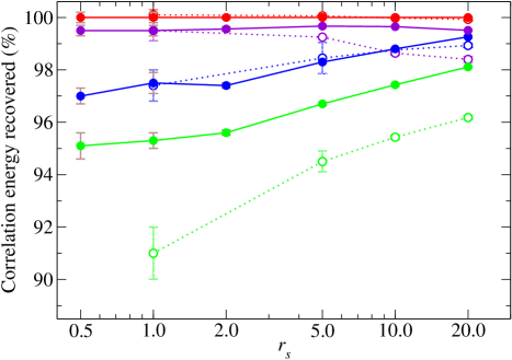
Figure 1: (Color online) Percentages of the correlation energy recovered at the (solid circles from top to bottom) BF-DMC, BF-VMC, SJ-DMC, and SJ-VMC levels as a function of the density parameter $r_{s}$ (see Table 1). Zero correlation energy corresponds to HF-VMC and 100% to BF-DMC. The hollow circles are the best BF-DMC, BF-VMC, SJ-DMC, and SJ-VMC energies of Holzmann et al.,holzmann_2003 in the same order. The statistical error bars on the QMC data are smaller than the symbols except where error bars are shown.

Figure 2: (Color online) VMC variances achieved at the SJ level (top solid line) and BF level (bottom solid line) as a function of the density parameter $r_{s}$ (see Table 1). The hollow circles are the best SJ-VMC and BF-VMC variances of Holzmann et al.,holzmann_2003 in the same order. The statistical error bars on the QMC data are smaller than the symbols except where error bars are shown.

The optimized homogeneous backflow displacement $\eta(r_{ij})r_{ij}$ is plotted in Figs. 3 and 4, and the optimized three-body function $w_{ij}$ is shown in Fig. 5. Holzmann et al.holzmann_2003  and Kwon et al.kwon_1998  used identical $\eta$ functions for parallel and antiparallel spin pairs, whereas we have allowed them to differ. At each density, the maximum value of $\eta(r_{ij})r_{ij}$ for antiparallel spins is over twice as large as that for parallel spins, and occurs at smaller electron separations. The backflow displacements for antiparallel spins are generally larger than for parallel spins, and hence antiparallel-spin backflow is much more important than parallel-spin backflow. Our antiparallel-spin $\eta$ function is similar to the spin-independent $\eta$ function of Kwon et al.,kwon_1998 except that we do not find an attractive tail at $r_{s}=20$. Note that, to obey the cusp conditions, we constrain the parallel-spin $\eta(r_{ij})$ function to have zero derivative at $r_{ij}=0$, while the antiparallel-spin $\eta$ function may have a nonzero derivative: see Appendix A.1. This accounts for the differences in the behavior of the parallel- and antiparallel-spin $\eta$ functions at small $r_{ij}$ which are visible in Figs. 3 and 4.

The magnitude of our optimized three-electron Jastrow factor, represented in Fig. 5, increases monotonically with $r_{s}$, and the maximum of $6(r_{ij}w_{ij})^{2}$ is at about $r_{ij}/r_{s}=0.4$ for all densities. This is in contrast with the behavior of the three-electron Jastrow factor of Kwon et al. (see Fig. 1 of Ref. kwon_1998, ), which changes sign at $r_{s}=1$ (our parametrization is not allowed to do so) and breaks its monotonicity with $r_{s}$ at $r_{s}=20$. Kwon et al. find that the maximum of the plotted function is located at about $r_{ij}/r_{s}=1$.

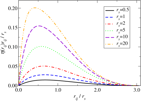
Figure 3: (Color online) Antiparallel-spin homogeneous backflow displacement $\eta(r_{ij})r_{ij}$ for the HEG at the different densities studied. For the three highest densities, the curves correspond to BF wave functions, while the others are for BF3 wave functions.

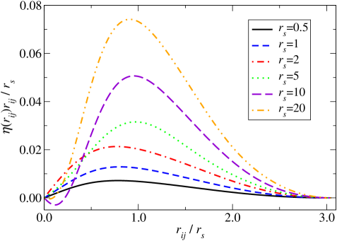
Figure 4: (Color online) Parallel-spin homogeneous backflow displacement $\eta(r_{ij})r_{ij}$ for the HEG at the different densities studied. For the three highest densities, the curves correspond to BF wave functions, while the others are for the BF3 wave function.

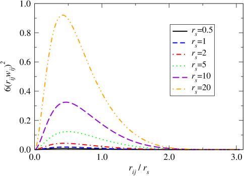
Figure 5: (Color online) Three-body contribution to the Jastrow function for the HEG due to three electrons at the vertices of an equilateral triangle of side $r_{ij}$, at the different densities studied. For the three highest densities, the curves correspond to SJ3 wave functions, while the other three are for BF3 wave functions.

IV.2 Lithium atom and dimer

IV.2.1 AE lithium atom

Our results for the ¹S ground state of the AE lithium atom are given in Table 2. The SJ wave function gives a reasonably good VMC energy. Our backflow function consists of a spin-pair-dependent e-e-n term with $N_{en}=N_{ee}=3$; this produces a BF-VMC energy that is within statistical error bars of the exact value. Note that the BF-VMC, SJ-DMC, and BF-DMC energies are within statistical error bars of each other and are very close to the exact value. The excellent performance of the BF-VMC calculation is particularly noteworthy. The single-determinant nodal surface of the ¹S ground state of lithium is certainly extremely accurate and may even be exact, although some contrary evidence has been cited.bressanini_2002 It is therefore unlikely that backflow could improve upon the SJ-DMC energy, and indeed it leaves it essentially unchanged.

Method	Wfn.	$N_{p}$	$E$ (a.u.)		$\sigma^{2}$ (a.u.)		% corr. en.
HF	-	-	$-7$.	$43273$	-		$0$.	$0$
Exact	-	-	$-7$.	$47806$	-		$100$.	$0$
VMC	SJ	0	$-7$.	$47648(3)$	$0$.	$00385(2)$	$96$.	$52(8)$
	BF	114	$-7$.	$47801(3)$	$0$.	$00241(1)$	$99$.	$89(6)$
DMC	SJ	0	$-7$.	$47803(8)$	-		$99$.	$9(2)$
	BF	114	$-7$.	$47802(6)$	-		$99$.	$9(1)$

Table 2: Slater-Jastrow and backflow results for the AE lithium atom. The number of free backflow parameters, excluding cutoff lengths, is $N_{p}$. The Hartree-Fock (HF) and exact energies were taken from Refs. davidson_1991, and chakravorty_1993, .

IV.2.2 AE lithium dimer

We studied the ground state of the AE ${\rm Li}_{2}$ dimer at the experimental bond length of $5.051$ a.u.cade_1974 We tested several different backflow functions, obtaining the results given in Table 3. The use of homogeneous backflow retrieves only an additional 0.7% of the correlation energy. A plot of the VMC energy as a function of the number of parameters is displayed in Fig. 6, which shows that the reduction in VMC energy is very small beyond about 150 parameters. Whereas backflow gave 99.89(6)% of the correlation energy at the VMC level for the lithium atom, for the dimer our best backflow transformation retrieves only 87.79(8)%. At the DMC level the improvement is small: using a SJ wave function we obtain 96.2(3)% of the correlation energy while with the backflow wave function this improves slightly [to 97.1(3)%]. Considerably better DMC results for ${\rm Li}_{2}$ have been obtained using multideterminant (MD) wave functions. Bressanini et al.bressanini_2005b  obtained a DMC energy of $-14.9923(2)$ with one configuration state function (CSF), while their best result was $-14.9952(1)$ with 4 CSFs.

Method	Wfn.	$N_{\eta}$	$N_{\mu}$	$N_{\rm en}$	$N_{\rm ee}$	$N_{p}$	$E$ (a.u.)		$\sigma^{2}$ (a.u.)		% corr. en.
HF	-	-	-	-	-	-	$-14$.	$871545$	-		$0$.	$0$
Exact	-	-	-	-	-	-	$-14$.	$9954$	-		$100$.	$0$
VMC	SJ	-	-	-	-	0	$-14$.	$9751(1)$	$0$.	$0165(1)$	$83$.	$6(1)$
	BF	0	6	0	0	14	$-14$.	$9755(1)$	$0$.	$01607(9)$	$83$.	$9(1)$
	BF	8	0	0	0	17	$-14$.	$9760(1)$	$0$.	$01590(7)$	$84$.	$3(1)$
	BF	0	0	2	2	16	$-14$.	$9768(1)$	$0$.	$01424(7)$	$84$.	$9(1)$
	BF	0	0	2	4	44	$-14$.	$9782(1)$	$0$.	$01273(7)$	$86$.	$15(9)$
	BF	0	0	2	6	72	$-14$.	$9789(1)$	$0$.	$0125(1)$	$86$.	$65(9)$
	BF	0	0	3	4	156	$-14$.	$9797(1)$	$0$.	$01102(5)$	$87$.	$33(8)$
	BF	0	0	4	4	308	$-14$.	$9802(1)$	$0$.	$01030(6)$	$87$.	$71(8)$
	BF	0	0	4	3	230	$-14$.	$9803(1)$	$0$.	$01038(4)$	$87$.	$79(8)$
DMC	SJ	-	-	-	-	0	$-14$.	$9907(4)$	-		$96$.	$2(3)$
	BF	0	0	4	3	230	$-14$.	$9918(4)$	-		$97$.	$1(3)$

Table 3: Slater-Jastrow and backflow results for the AE ${\rm Li}_{2}$ molecule. The different backflow forms have been put in order of decreasing energy. The number of free backflow parameters, excluding cutoff lengths, is $N_{p}$. The Hartree-Fock (HF) and exact energies were taken from Ref. filippi_1996, .

Figure 6: The VMC energy of AE ${\rm Li}_{2}$ versus the total number of parameters in the backflow functions.

The computed binding energies of ${\rm Li}_{2}$ are presented in Table 4. The BF-VMC, SJ-DMC, and BF-DMC energies of the AE lithium atom are within error bars of the exact energy, and therefore the error in the binding energy arises solely from the ${\rm Li}_{2}$ energy. Backflow improves the VMC and DMC binding energies of ${\rm Li}_{2}$ a little, but it is still somewhat short of the exact value. The single-determinant nodal surface of ${\rm Li}_{2}$ is quite poor, and backflow is not very effective at improving it. Combining MD wave functions with backflow might yield significant improvements in this case.

Method	Wfn.	$E_{b}$ (a.u.)
HF	-	$0$.	$0061$
Exact	-	$0$.	$0393$
VMC	SJ	$0$.	$0221(1)$
	BF	$0$.	$0243(1)$
DMC	SJ	$0$.	$0346(4)$
	BF	$0$.	$0358(4)$

Table 4: Slater-Jastrow and backflow binding energies for the AE ${\rm Li}_{2}$ molecule, computed using the best results from Tables 2 and 3. The Hartree-Fock (HF) and exact energies were taken from Refs. davidson_1991, , chakravorty_1993, , and filippi_1996, , and references therein.

IV.3 Carbon atom, carbon dimer, and diamond

IV.3.1 AE carbon atom

The ³P ground state of the AE carbon atom is a good example of a system where single-determinant wave functions result in large fixed-node errors: see Table 5. In this case, we have tested several combinations of terms, expansion orders, and constraints to explore the possibilities of backflow transformations. The VMC data in Table 5, and additional data, are plotted in Fig. 7, where the performance of the different backflow functions used can be compared conveniently. Using only homogeneous backflow (first BF-VMC results in Table 5) gives a very small reduction in energy. It seems that inhomogeneous systems require inhomogeneous backflow to produce good wave functions, and the e-e-n term is particularly successful in providing this. To evaluate the relative importance of the two e-e-n functions $\Phi_{i}^{jI}$ and $\Theta_{i}^{jI}$, we performed calculations constraining the parameters in one of them to be zero. The results are also given in Table 5. In this case $\Theta_{i}^{jI}$, which contributes to the backflow displacement in the direction of ${\bf r}_{iI}$, is slightly more important than $\Phi_{i}^{jI}$. Applying both terms gives better results than using only one of them, as we expected. We also tested the effect of constraining the backflow displacement to be irrotational, which was suggested in Ref. holzmann_2003, . The application of this constraint, which is explained in Appendix A.2, approximately halves the number of parameters in the backflow functions, but it gives very poor results for the carbon atom.

Method	Wfn.	$N_{\eta}$	$N_{\mu}$	$N_{\Phi}$	S	I	$N_{p}$	$E$ (a.u.)		$\sigma^{2}$ (a.u.)		% corr. en.
HF	-	-	-	-	-	-	-	$-37$.	$688619$	-		$0$.	$0$
Exact	-	-	-	-	-	-	-	$-37$.	$8450$	-		$100$.	$0$
VMC	SJ	-	-	-	-	-	0	$-37$.	$8064(3)$	$0$.	$193(2)$	$75$.	$3(2)$
	BF	8	0	0	T	-	17	$-37$.	$8089(3)$	$0$.	$194(2)$	$76$.	$9(2)$
	BF	0	6	0	T	-	10	$-37$.	$8089(3)$	$0$.	$184(1)$	$76$.	$9(2)$
	BF	0	0	2	F	F	10	$-37$.	$8119(3)$	$0$.	$1685(8)$	$78$.	$8(2)$
	BF	8	6	0	T	-	27	$-37$.	$8126(3)$	$0$.	$178(2)$	$79$.	$3(2)$
	BF	0	0	4	T	T	35	$-37$.	$8140(3)$	$0$.	$171(2)$	$80$.	$2(2)$
	BF†	0	0	3	T	F	56	$-37$.	$8155(3)$	$0$.	$1578(9)$	$81$.	$1(2)$
	BF	0	0	5	T	T	121	$-37$.	$8177(3)$	$0$.	$153(2)$	$82$.	$5(2)$
	BF	0	0	2	T	F	16	$-37$.	$8180(3)$	$0$.	$159(4)$	$82$.	$7(2)$
	BF‡	0	0	3	T	F	58	$-37$.	$8198(3)$	$0$.	$144(2)$	$83$.	$7(2)$
	BF	0	0	3	F	F	60	$-37$.	$8225(3)$	$0$.	$135(2)$	$85$.	$5(2)$
	BF	0	0	4	F	F	158	$-37$.	$8239(3)$	$0$.	$119(6)$	$86$.	$5(2)$
	BF	0	0	3	T	F	114	$-37$.	$8246(3)$	$0$.	$127(2)$	$87$.	$0(2)$
	BF	0	6	3	T	F	124	$-37$.	$8252(3)$	$0$.	$122(1)$	$87$.	$3(2)$
	BF	0	0	4	T	F	308	$-37$.	$8259(3)$	$0$.	$109(1)$	$87$.	$8(2)$
DMC	SJ	-	-	-	-	-	0	$-37$.	$8297(2)$	-		$90$.	$2(1)$
	BF	0	6	3	T	F	124	$-37$.	$8324(1)$	-		$92$.	$0(1)$

Table 5: Slater-Jastrow and backflow results for the AE carbon atom. The different backflow forms have been put in order of decreasing energy. Key: $N_{\Phi}\equiv N_{\rm en}=N_{\rm ee}$; S indicates whether the parameters are spin and spin-pair dependent (T) or not (F); I indicates whether the constraints for irrotational backflow have been applied (T) or not (F); $N_{p}$ is the number of free backflow parameters, excluding cutoff lengths. Where the † symbol is used, we constrained $\theta_{klm,I}=0$; where the ‡ symbol appears, we constrained $\varphi_{klm,I}=0$. The Hartree-Fock (HF) and exact energies were taken from Refs. davidson_1991, and chakravorty_1993, .

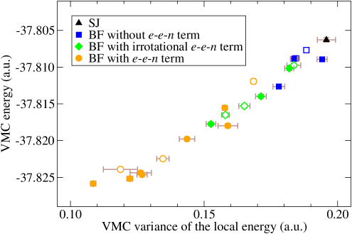
Figure 7: (Color online) The VMC energy versus its variance for AE carbon (see Table 5). The open symbols denote that the backflow parameters are independent of spin, while the filled symbols denoted spin-dependent parameters. The exact nonrelativistic energy is $-37.8450$ a.u.davidson_1991 ; chakravorty_1993

The most satisfactory backflow forms reduce the difference between the VMC and exact energies by a factor of about 2. The further energy reduction from using DMC is quite small, and our BF-DMC calculation gave an energy of $-37.8324(1)$ a.u., which corresponds to 92.0(1)% of the total correlation energy. This suggests that, although backflow improves significantly upon the single-determinant nodal surface of the carbon atom, it misses some important features of the exact nodal surface. It is well-known that the single-determinant nodal surface of the carbon atom can be substantially improved by using MD trial wave functions. Barnett et al.barnett_2000  used an MD trial wave function consisting of 14 CSFs, and obtained a DMC energy of $-37.8420(3)$ a.u., which corresponds to 98.1(2)% of the correlation energy. Glauser et al.glauser_1992  showed that the configuration space of a single-determinant of HF orbitals for the ³P ground state carbon atom is divided into four nodal pockets, but more accurate wave functions indicate that the exact wave function has two nodal pockets. It appears that backflow transformations are unable to correct this defect in the single-determinant nodal surface.

IV.3.2 PP carbon atom

We have also studied how backflow performs in systems where PPs are used. Our results for a PP carbon atom are given in Table 6. The reduction in the VMC energy obtained with backflow is much smaller than for the AE carbon atom, but the corresponding energy reduction within DMC of $0.0039(1)$ a.u. is somewhat larger than the AE one of $0.0027(2)$ a.u. A peculiarity of this case is that the reduction in the DMC energy resulting from the use of backflow is $71\%$ of the reduction in the VMC energy, which is the largest such percentage amongst the calculations described here.

Method	Wfn.	$N_{p}$	$E$ (a.u.)		$\sigma^{2}$ (a.u.)		% corr. en.
HF	-	-	$-5$.	$31663$	-		$0$	$.0$
Exact	-	-	$-5$.	$420(4)$	-		$100$	$(8)$
VMC	SJ	0	$-5$.	$4007(1)$	$0$.	$0582(4)$	$81$	$(3)$
	BF	218	$-5$.	$4061(1)$	$0$.	$0502(6)$	$87$	$(3)$
DMC	SJ	0	$-5$.	$40886(7)$	-		$89$	$(4)$
	BF	218	$-5$.	$41273(9)$	-		$93$	$(4)$

Table 6: Slater-Jastrow and backflow results for the PP carbon atom. The number of free backflow parameters, excluding cutoff lengths, is $N_{p}$. The exact energy was taken from Ref. dolg_1996, .

IV.3.3 PP carbon dimer

For the PP carbon dimer we used the experimental bond length of $2.3622$ a.u.,cade_1974 obtaining the results given in Table 7. The carbon dimer is another example of a system in which MD effects are known to be substantial. Backflow results in larger energy reductions per atom than for the isolated atom at both the VMC and DMC levels. The computed binding energies of ${\rm C}_{2}$ are presented in Table 8. The use of backflow slightly improves the binding energy of the dimer.

Method	Wfn.	$N_{p}$	$E$ (a.u.)		$\sigma^{2}$ (a.u.)		% corr. en.
HF	-	-	$-10$.	$652399$	-		$0$	$.0$
Exact	-	-	$-11$.	$055(4)$	-		$100$	$(2)$
VMC	SJ	0	$-10$.	$9870(3)$	$0$.	$168(1)$	$83$	$.1(9)$
	BF	214	$-11$.	$0173(2)$	$0$.	$156(2)$	$91$	$(1)$
DMC	SJ	0	$-11$.	$0237(4)$	-		$92$	$(1)$
	BF	214	$-11$.	$0348(6)$	-		$95$	$(1)$

Table 7: Slater-Jastrow and backflow results for the PP ${\rm C}_{2}$ molecule. The number of free backflow parameters, excluding cutoff lengths, is $N_{p}$. The exact energy was taken from Ref. dolg_1996, .

Method	Wfn.	$E_{b}$ (a.u.)
HF	-	$0$.	$02896$
Exact	-	$0$.	$233(5)$
VMC	SJ	$0$.	$1856(3)$
	BF	$0$.	$2051(2)$
DMC	SJ	$0$.	$2060(4)$
	BF	$0$.	$2093(6)$

Table 8: Slater-Jastrow and backflow binding energies for the PP ${\rm C}_{2}$ molecule, computed using the results from Tables 6 and 7. The Hartree-Fock (HF) and exact energies were taken from Refs. davidson_1991, , chakravorty_1993, , and filippi_1996, , and the references therein. The data in Ref. dolg_1996, can be used to estimate an approximate binding energy of $0.215(6)$ a.u..

IV.3.4 PP diamond

We have also studied PP carbon diamond with the experimental cubic lattice constant of $6.741$ a.u.,sato_2002 representing the solid by a $2\times 2\times 2$ supercell containing 16 atoms subject to periodic boundary conditions. Diamond is an insulator with a large band gap, and therefore we expect the single-determinant nodal surface to be quite accurate. We parametrized our backflow function using $N_{\eta}=8$, $N_{\mu}=8$, and $N_{\rm ee}=N_{\rm en}=2$, allowing all parameters to be spin and spin-pair dependent. The cutoff lengths were optimized, and they went to the maximum allowed values. The results in Table 9 show that backflow gives a substantial reduction in the VMC energy of $0.0131(2)$ a.u. per atom [$0.356(5)$ eV per atom], which is accompanied by a reduction in the variance by a factor of nearly two. The reduction in the VMC energy of diamond from using backflow is somewhat smaller than that obtained in the dimer [$0.411(5)$ eV per atom], and substantially larger than that in the atom [$0.147(3)$ eV per atom]. This may arise from the fact that the backflow functions in diamond are quite long ranged and cover several atoms. Backflow reduces the DMC energy of diamond by $0.0035(2)$ a.u. [$0.095(5)$ eV per atom] per atom, which is a little less than in the dimer [$0.15(1)$ eV per atom] and atom [$0.106(3)$ eV per atom].

Method	Wfn.	$N_{p}$	$E$ (a.u./prim. cell)		$\sigma^{2}$ (a.u.)
DFT-PBE	-	-	$-11$.	$368208$	-
VMC	SJ	0	$-11$.	$3708(2)$	$1$.	$51(8)$
	BF	96	$-11$.	$3970(3)$	$0$.	$897(8)$
DMC	SJ	0	$-11$.	$40717(8)$	-
	BF	96	$-11$.	$4141(3)$	-

Table 9: Slater-Jastrow and backflow energies per primitive cell for PP carbon diamond using a face-centered cubic cell containing 16 atoms. The number of free backflow parameters, excluding cutoff lengths, is $N_{p}$.

We do not discuss the cohesive energy of the diamond crystal, as we would need to account for finite-size effects to be able to compare with experimental data. Within VMC, the energy gain per atom from using backflow is larger in the solid than in the atom, and hence the cohesive energy is substantially reduced. Within DMC, both the solid and the atom present a similar energy gain per atom, and the cohesive energy is not changed significantly.

V Discussion

V.1 Electron-by-electron and configuration-by-configuration algorithms

The additional complexity of BF wave functions compared with SJ ones leads to greater computational expense in QMC calculations. One of the most costly operations in QMC calculations is the evaluation of the orbitals and their first two derivatives at points in the configuration space. The evaluation of the collective coordinates involves some extra cost. Furthermore, while QMC calculations with SJ wave functions require only the value, gradient, and Laplacian of each orbital $\phi$, calculations with BF wave functions also require cross derivatives such as $\partial^{2}\phi/\partial x\partial y$, as explained in Ref. kwon_1993, . However, the most important complicating factor arising from backflow transformations is that they make each orbital in the Slater determinants depend on the coordinates of every particle. In standard QMC algorithms with SJ wave functions one moves the electrons sequentially in what we call the electron-by-electron algorithm (EBEA). Fast update algorithms are used in the EBEA to replace altered rows in the Slater determinants efficiently and the accept/reject step is performed on each particle separately. However, in BF calculations each collective coordinate depends on every electron position and therefore the fast update algorithms used in the EBEA are no longer appropriate, so that one must recalculate the determinants at each step using LU decomposition. Nevertheless, the implementation of the EBEA for backflow wave functions can take advantage of other optimizations to make the algorithm more efficient, such as buffering the separate contributions to the collective coordinates, which we have exploited as far as possible.

In previous fermion backflow calculationskwon_1993 ; kwon_1998 ; holzmann_2003 the electrons have all been moved together and a single accept/reject step has been performed, in what we call the configuration-by-configuration algorithm (CBCA). We have compared the efficiency of the EBEA and CBCA. The relative efficiency of the EBEA and CBCA depends on the computational costs of moving the electrons and the correlation time of the local energies, which is proportional to the number of moves of all the electrons required before the local energies are uncorrelated. Let A and B be two calculations for the same system, identical except for the use of different sampling algorithms. We define the relative efficiency $\gamma$ of A and B as

$$\gamma({\rm A},{\rm B})=\frac{t_{\rm A}\sigma_{\rm A}^{2}}{t_{\rm B}\sigma_{\rm B}^{2}}\;,$$ (14)

where $t$ is the CPU time and $\sigma$ is the standard error in the mean energy.flyvbjerg_1989 $\gamma$ represents the ratio of the time required to achieve a fixed error in the mean energy in calculation A to that required in calculation B, and is hence appropriate for comparing the efficiency of the two algorithms.

In Table 10 we report results for the systems studied in this paper. For each system, the EBEA and CBCA time steps were chosen so that the same proportion of proposed moves were accepted: in VMC the target acceptance ratio was 50%, which corresponds to fairly efficient sampling, and in DMC it was around 99.5%. The correlation times for the CBCA are considerably longer than for the EBEA. The ratio of the correlation time of the CBCA to that of the EBEA (the “correlation time ratio” or CTR) appears to increase roughly linearly with the number of atoms (for example, compare the AE Li atom and ${\rm Li}_{2}$ molecule, and the PP C atom, ${\rm C}_{2}$ molecule, and diamond), or with the number of electrons. $\gamma({\rm CBCA},{\rm EBEA})$ is larger than unity in all cases except the BF-VMC calculation of lithium atom, so the EBEA is generally found to be more efficient than the CBCA. $\gamma({\rm CBCA},{\rm EBEA})$ is larger for SJ wave functions than for BF ones because for SJ wave functions and the EBEA one uses fast update algorithms.

System	$N_{e}$	Wfn	CTR.	$\gamma_{\rm VMC}$		$\gamma_{\rm DMC}$
HEG ($r_{s}=1.0$)	54	SJ	70	44.	0	7.	5
		BF		34.	0	1.	2
AE Li atom	3	SJ	9	4.	6	1.	8
		BF	1	0.	43	1.	9
AE ${\rm Li}_{2}$ molecule	6	SJ	15	15.	4	5.	0
		BF		9.	9	3.	8
AE C atom	6	SJ	9	5.	1	7.	9
		BF	3	2.	4	3.	7
PP C atom	4	SJ	3	3.	3	3.	7
		BF	2	2.	3	1.	3
PP ${\rm C}_{2}$ molecule	8	SJ	10	6.	9	3.	5
		BF		6.	9	1.	5
PP C diamond	64	SJ	80	99.	0	-
($2\times 2\times 2$)		BF		39.	0	-

Table 10: Comparison of the EBEA and CBCA for SJ and BF wave functions. Key: $N_{e}$ is the number of electrons; “CTR” is the ratio of the correlation time in the CBCA to that in the EBEA; $\gamma$ is $\gamma$(CBCA,EBEA), as defined in Eq. (14). Where a separate “CTR” for the BF wave function has not been reported, it is because it was found to equal that of the SJ wave function.

Apart from the tests reported in this section, all the VMC and DMC results reported in this paper have been obtained using the EBEA.

V.2 Computational expense of backflow calculations

We now investigate the relative cost of BF and SJ calculations. The additional computational expense of each step in a BF calculation is offset by the fact that BF wave functions are generally more accurate than SJ ones, so that the variance of the energy is smaller, and consequently the number of statistically independent local energies required to achieve a given error bar in the mean energy is also smaller.

Let A and B be two calculations for the same system, identical except for the use of different wave functions. We define the time ratio as $\tau({\rm A},{\rm B})=t_{\rm A}/t_{\rm B}$, the squared-error ratio as $\epsilon({\rm A},{\rm B})=\sigma_{\rm A}^{2}/\sigma_{\rm B}^{2}$, and the relative efficiency as $\gamma({\rm A},{\rm B})=\tau({\rm A},{\rm B})\epsilon({\rm A},{\rm B})$, where $t$ is the CPU time and $\sigma$ is the standard error in the mean energy. $\tau({\rm A},{\rm B})$ represents the relative expense per move of calculation A with respect to calculation B or, equivalently, the relative expense of generating a fixed number of configurations. The latter is relevant to the wave-function optimization procedure, as the number of configurations used should, if anything, increase with the number of parameters in the wave function. $\gamma({\rm A},{\rm B})$ measures the relative ability of calculation A to produce a total energy to a desired degree of certainty with respect to B.

In Table 11 we compile the BF-to-SJ ratios $\tau$, $\epsilon$, and $\gamma$ for each calculation. For the HEG at $r_{s}=20$ we report BF3-to-SJ3 ratios instead. The performance of backflow in the HEG is impressive: backflow not only improves the energies but also makes the calculations less costly!

The lithium atom is another example of improved efficiency. According to Table 2, the SJ-DMC and BF-DMC energies are equal, so it does not seem advantageous to use backflow at all in this system. However, due to the BF-VMC energy being so close to the BF-DMC value, the variance of the BF-DMC run is enormously lowered and the CPU time is reduced to $25\%$ of the time taken by the SJ-DMC run.

In all cases except PP diamond, $\gamma$ is less than $3$ in VMC, and $6$ in DMC. However, the crystalline PP calculations become significantly more expensive when backflow is used. A great part of this increase is due to the computation of the nonlocal PP energy, which involves several evaluations of the wave function ($12$, in this case) for each electron and each ion, every time the local energy is computed.

System	$N_{e}$	Method	$\tau$		$\epsilon$		$\gamma$
HEG ($r_{s}=1.0$)	54	VMC	2.	9	0.	18	0.	52
		DMC	4.	9	0.	15	0.	75
HEG ($r_{s}=20.0$)	54	VMC	1.	4	0.	48	0.	67
		DMC	2.	0	0.	15	0.	28
AE Li atom	3	VMC	2.	3	0.	52	1.	2
		DMC	4.	3	0.	06	0.	25
AE ${\rm Li}_{2}$ molecule	6	VMC	3.	9	0.	71	2.	8
		DMC	8.	3	0.	71	5.	9
AE C atom	6	VMC	3.	5	0.	69	2.	4
		DMC	5.	9	0.	41	2.	4
PP C atom	4	VMC	3.	1	0.	79	2.	4
		DMC	2.	8	0.	73	2.	1
PP ${\rm C}_{2}$ molecule	8	VMC	3.	9	0.	65	2.	5
		DMC	3.	3	0.	47	1.	6
PP C diamond	64	VMC	27.	0	0.	31	8.	3
($2\times 2\times 2$)		DMC	-		-		-

Table 11: Data from the timing tests performed on different systems. Key: $N_{e}$ is the number of electrons; $\tau$, $\epsilon$, and $\gamma$ are $\tau$(BF,SJ), $\epsilon$(BF,SJ), and $\gamma$(BF,SJ), as defined in the text.

V.3 Backflow and nodes

HF nodes have been compared with either exact or very accurate nodes in a number of studies.glauser_1992 ; bressanini_2002 ; bressanini_2005a ; bressanini_2005b ; bajdich_2005 It has been found that the HF wave function often has too many nodal pockets for the ground states of atoms with four or more electrons. It is conceivable that coordinate transformations could modify the number of nodal pockets of a wave function. However, we believe this to be unlikely for the backflow transformation presented in this paper, because this would require the backflow displacement field to be discontinuous at very specific configurations, or exhibit other unusual features. The development of a general backflow transformation with the appropriate discontinuities to correct HF nodes, which we have not attempted, seems likely to be a tremendously difficult task.

We now illustrate graphically how our backflow transformations changes nodal surfaces. Note that the figures described below are single projections of high-dimensional nodal surfaces, from which almost no useful conclusions regarding the full topology of the nodes can be extracted. Two-dimensional projections of the HF and BF nodes for a two-dimensional HEG are depicted in Fig. 8 at two different densities. The effect of backflow on the nodes is much more pronounced for the low-density HEG. For an unpolarized system, the nodal changes should be larger than those seen in Fig. 8 at all densities. Some regions of these plots suggest that the displacement of the nodes due to backflow is largest at points where the curvature of the nodal surface is large, away from electron-electron coalescences. There are a number of avoided crossings in Fig. 8 (3 at $r_{s}=0.5$, and 6 at $r_{s}=10$) whose connectivity (in the projection) is modified by backflow.

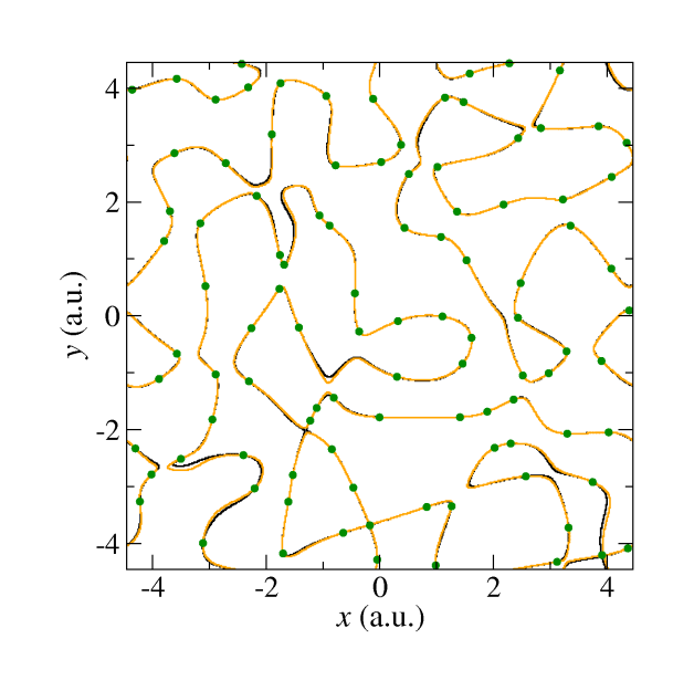
(a)  Nodes in a 2D HEG at $r_{s}=0.5$.

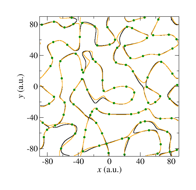
(b)  Nodes in a 2D HEG at $r_{s}=10$.

Figure 8: (Color online) Nodes encountered when moving one of the electrons of a two-dimensional HEG of 101 like-spin electrons at two different densities. The HF and BF nodes are in black and orange, respectively. The green circles indicate the positions of the remaining 100 electrons, at which the nodes are required to remain fixed. The backflow wave functions were obtained by variance minimization; the energy reductions from SJ-VMC to BF-VMC at $r_{s}=0.5$ and $10$ were $0.0007(1)$ a.u./electron and $0.00005(1)$ a.u./electron, respectively.

Three-dimensional projections of the HF and BF nodes of the AE carbon atom are compared in Fig. 9. The nodes are substantially modified by the introduction of backflow. New nodal regions appear in this projection because the electron being moved “pushes” the other electrons (via the backflow transformation) through the nodal surface of the HF wave function.

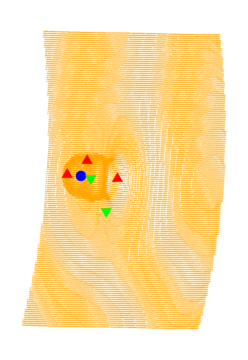
(a)  HF nodes of a carbon atom.

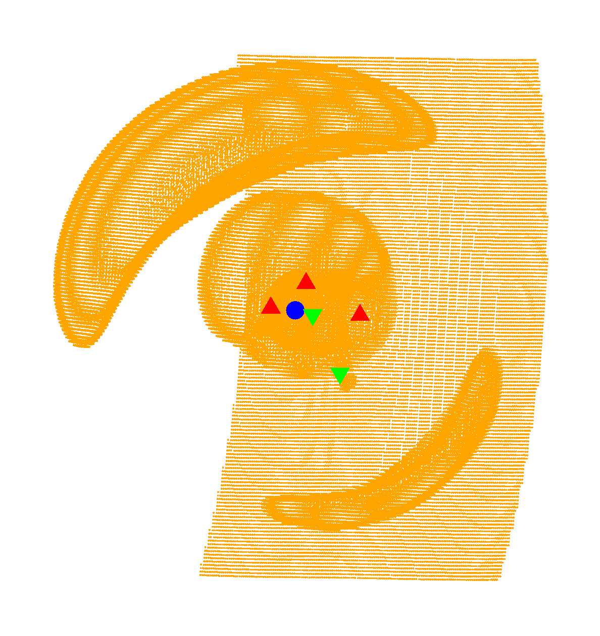
(b)  BF nodes of a carbon atom.

Figure 9: (Color online) HF and BF nodes encountered when moving one of the (majority spin) up-spin electrons of an AE carbon atom. The blue circle corresponds to the position of the nucleus, the red upward-pointing triangles indicate the positions of the remaining up-spin electrons and the green downward-pointing triangles indicate the positions of the down-spin ones. The HF node consists of a (seemingly) infinite sheet with a bubble attached to it, which contains the nucleus. Backflow slightly modifies this node, and adds three large lobes (detached from one another; all intersect the HF node) and a small bubble next to a down-spin electron.

VI Conclusions

We have devised an inhomogeneous backflow transformation for systems consisting of electrons and either nuclei or ions represented by pseudopotentials. We have applied our backflow transformation to single-determinant Slater-Jastrow wave functions for the HEG and for atomic, molecular, and solid systems. In each case backflow gives a substantial reduction in the VMC energy, and a smaller reduction in the DMC energy.

The homogeneous backflow transformation reduces the variance of the VMC energy of the HEG by a factor of about 4, which is the largest such factor we have encountered, and we believe that our backflow wave functions for the HEG are very accurate. VMC retrieves more than 99.5% of the DMC correlation energy in the density range studied ($r_{s}=0.5$–20). The effects of backflow on the nodes increase with $r_{s}$, even though the additional percentage of the correlation energy retrieved in VMC decreases with $r_{s}$, implying that the energies of dilute HEGs are less sensitive to the nodal structure of the trial wave function than those of denser systems.

Although backflow works very well in the HEG, as previous studies have already concluded, we find that purely homogeneous backflow transformations give poor results when atoms are present, as we demonstrated for the AE lithium dimer and the AE carbon atom. However, in these cases inhomogeneous backflow transformations can improve the wave functions substantially.

For the AE lithium atom the HF nodal surface of the SJ wave function is essentially exact. Although in this case backflow cannot improve the DMC energy, it gives a very accurate VMC energy. This shows that backflow transformations can improve the wave function away from the nodes as well as improving the nodal surface itself. The quality of the SJ and BF wave functions for the AE lithium dimer are much lower than for the atom, and consequently the binding energy of the dimer is underestimated. The wave function and nodal surface of the AE lithium dimer can be substantially improved by using several determinants,bressanini_2005b but it appears that only modest improvements can be obtained using backflow.

Backflow reduces the VMC energy of the AE carbon atom by about 49% of the correlation energy missing at the SJ-VMC level, but at the DMC level the improvement is smaller; the BF-DMC energy is only 18% closer to the exact value than SJ-DMC. Backflow makes a more significant improvement to the DMC energy of a PP carbon atom than the AE carbon atom. The PP and AE carbon atoms are also cases where substantial improvements to the wave functions can be obtained by using several determinants. This indicates that the SJ nodal surfaces of these two systems need a more drastic correction than backflow transformations can provide.

When the initial nodal surface is reasonably accurate, backflow does an excellent job in improving the VMC energy and correcting the remaining errors in the nodal surface, as was seen in our study of the HEG and AE lithium. However, when the initial nodal surface is intrinsically poor, as is the case, for example, with the HF nodal surfaces of the carbon atom and dimer, backflow is apparently incapable of making the gross changes to the nodal surface required to correct the flaws, although it normally lowers the VMC and DMC energies somewhat. We do not believe that our backflow transformation is capable of changing the number of nodal pockets of the starting wave function.

The cost of using BF wave functions can be substantial, but we have given evidence that the expense relative to that of using SJ wave functions increases smoothly with the number of atoms in the system. Backflow transformations, like Jastrow factors and unlike multideterminant expansions, are compact parametrizations, meaning that the number of parameters required to retrieve a given fraction of the correlation energy increases only slowly with system size. This can be seen by comparing the number of backflow parameters that we have used and the energies we have obtained for PP carbon atom, dimer, and diamond. We have found that it is much more efficient to move electrons one at a time (the EBEA) than to move all the electrons at once (the CBCA), as has been done in previous backflow calculations. The reason for this is that the correlation time of the energy is considerably shorter with the EBEA. It is important to use the EBEA for large systems, as the CBCA-to-EBEA ratio of correlation times seems to increase linearly with the number of electrons.

BF-VMC energies are normally significantly lower than SJ-VMC ones, and therefore BF-VMC might be a useful alternative to a (normally more expensive) SJ-DMC calculation. The use of more accurate trial wave functions improves the statistical efficiency of VMC and DMC calculations. The variance of the local energies encountered in a DMC calculation is approximately proportional to the error in the VMC energy, and when backflow leads to a significant reduction in the VMC energy it also improves the statistical efficiency of DMC calculations, even when backflow improves the DMC energy only slightly. The improved trial wave functions could also be useful in DMC calculations of quantities other than the energy, which are normally more difficult to obtain accurately than the energy.

Backflow would appear to give significant improvements in trial wave functions for a wide variety of systems, including various different atoms, and small and large systems. In the present work, we have applied the inhomogeneous backflow transformation to single-determinant Slater-Jastrow wave functions only, but it can be combined with multideterminant wave functions, and we will report on such calculations elsewhere.trail_2006 It can also be combined with pairing wave functions.lopez_rios_2006 We believe that inhomogeneous backflow transformations will play an important role in improving trial wave functions for use in VMC and DMC calculations.

VII Acknowledgments

Financial support has been provided by the Engineering and Physical Sciences Research Council of the United Kingdom. P.L.R. acknowledges the financial support provided through the European Community’s Human Potential Programme under contract HPRN-CT-2002-00298, RTN “Photon-Mediated Phenomena in Semiconductor Nanostructures.” N.D.D. acknowledges financial support from Jesus College, Cambridge. M.D.T. acknowledges financial support from the Royal Society. Computer resources have been provided by the Cambridge-Cranfield High Performance Computing Facility.

Appendix A Constraints on the backflow parameters

A.1 Cusp conditions

The Kato cusp conditionskato ; pack (KCC) are enforced so that the local energy is finite when two electrons or an electron and a nucleus are coincident. For SJ wave functions it is common practice to impose the electron-electron KCC (EKCC) by constraining the parameters in the Jastrow function, and the electron-nucleus KCC (NKCC) by constraining the orbitals in the Slater determinant. The backflow transformation can alter the nature of the cusps, but we have chosen to constrain the backflow parameters so that they do not modify the KCC as applied to the Slater-Jastrow wave function.

Let $i$ and $j$ be two different electrons in the system. To satisfy the EKCC, we require that the total backflow displacement $\mbox{\boldmath$\xi$}_{i}$, has a well-defined gradient (i.e. it should be cuspless) when $r_{ij}\rightarrow 0$ if $i$ and $j$ are distinguishable particles, and have zero gradient when $r_{ij}\rightarrow 0$ if $i$ and $j$ are indistinguishable. Thus, the e-e term is affected by these constraints only if $i$ and $j$ are like-spin electrons, in which case the EKCC are satisfied if $L_{\eta}c_{1}=Cc_{0}$.

Let $I$ be a nucleus in the system. To satisfy the NKCC, we require that the total backflow displacement, $\mbox{\boldmath$\xi$}_{i}$, has a well-defined gradient when $r_{iI}\rightarrow 0$, and that it is zero when $r_{iI}\rightarrow 0$ if $I$ is an AE atom. The NKCC are satisfied if $L_{\mu,I}d_{1,I}=Cd_{0,I}$ for all $I$, and in addition, $d_{0,I}=0$, if $I$ is an AE atom.

The constraints on the e-e-n functions, some of which only apply to those functions centered on AE atoms, are as follows. (We omit the $I$ index in the parameters for clarity.)

• There are $3\left(N_{\rm ee}+N_{\rm en}+1\right)$ constraints from the NKCC,

  $$\sum_{l,m}^{(l+m=\alpha)}\left(C\varphi_{0lm}-L_{\Phi}\varphi_{1lm}\right)=\sum_{k,m}^{(k+m=\alpha)}\left(C\varphi_{k0m}-L_{\Phi}\varphi_{k1m}\right)=\sum_{k,m}^{(k+m=\alpha)}\left(C\theta_{k0m}-L_{\Phi}\theta_{k1m}\right)=0\;\;\;\;\forall~{}\alpha\;.$$ (15)

• There are $2N_{\rm en}+1$ constraints from the EKCC,

  $$\sum_{k,l}^{(k+l=\alpha)}\theta_{kl1}=0\;\;\;\;\forall~{}\alpha\;,$$ (16)

  and $2N_{\rm en}+1$ extra constraints for like-spin electron pairs,

  $$\sum_{k,l}^{(k+l=\alpha)}\varphi_{kl1}=0\;\;\;\;\forall~{}\alpha\;.$$ (17)

• [AE only] There are $4\left(N_{\rm ee}+N_{\rm en}\right)+2$ constraints on $\varphi_{klm}$,

  $$\sum_{l,m}^{(l+m=\alpha)}\varphi_{0lm}=\sum_{l,m}^{(l+m=\alpha)}m\varphi_{0lm}=\sum_{k,m}^{(k+m=\alpha)}\varphi_{k0m}=\sum_{k,m}^{(k+m=\alpha)}m\varphi_{k0m}=0\;\;\;\;\forall~{}\alpha\;.$$ (18)

• [AE only] There are $3\left(N_{\rm ee}+N_{\rm en}\right)+2$ constraints on $\theta_{klm}$,

  $$\sum_{l,m}^{(l+m=\alpha)}\theta_{0lm}=\sum_{l,m}^{(l+m=\alpha)}m\theta_{0lm}=\sum_{k,m}^{(k+m=\alpha)}m\theta_{k0m}=0\;\;\;\;\forall~{}\alpha\;.$$ (19)

These constraints form an indeterminate system of homogeneous algebraic linear equations for the e-e-n parameters. Hence, a subset of the parameters can be put in terms of the rest. This subset can be determined from the “free” parameters by putting the constraints in matrix form and using Gaussian elimination. This procedure is the one described in Ref. drummond_2004, , where it is applied to the parameters in the e-e-n term of the Jastrow factor.

A.2 Constraints for irrotational backflow

In the derivation of homogeneous backflow in Ref. holzmann_2003, it was suggested that the backflow displacement should satisfy $\mbox{\boldmath$\xi$}_{i}=\nabla_{i}Y$, where $Y=Y({\bf R})$ is an object called the backflow potential. This equation is already satisfied by both the e-e and e-n terms, by definition, and it can be imposed on the e-e-n functions by using an appropriate set of constraints. From $\nabla_{i}\times\mbox{\boldmath$\xi$}_{i}={\bf 0}$, it follows that

$$r_{ij}\frac{\partial}{\partial r_{iI}}\left[\Phi_{i}^{jI}f(r_{iI};L_{\Phi,I})\right]=r_{iI}\frac{\partial}{\partial r_{ij}}\left[\Theta_{i}^{jI}f(r_{iI};L_{\Phi,I})\right]\;,$$ (20)

for all $i$, $j$, and $I$, and all $r_{ij}$, $r_{iI}$, and $r_{jI}$. For $C>0$, this results in the equation

$$\left(C+k\right)\varphi_{k,l,m-1}-L_{\Phi}\left(k+1\right)\varphi_{k+1,l,m-1}-\left(m+1\right)\theta_{k-2,l,m+1}+L_{\Phi}\left(m+1\right)\theta_{k-1,l,m+1}=0\;,$$ (21)

while for $C=0$,

$$\left(k+1\right)\varphi_{k+1,l,m-1}-\left(m+1\right)\theta_{k-1,l,m+1}=0\;.$$ (22)

In both cases, $0\leq k\leq N_{\rm en}+2$, $0\leq l\leq N_{\rm en}$, and $0\leq m\leq N_{\rm ee}+1$, and parameters with indices out of the allowed range are to be taken as equal to zero. The $I$ index has been omitted for clarity.

The application of these constraints results in a reduction in the number of free parameters by more than one half, as one would expect, because an equivalent backflow displacement would be obtained by parameterizing the scalar field $Y$ and computing its gradient, whereas we use two scalar fields in the full e-e-n term.

Appendix B Zeroing the backflow displacement at AE atoms

When AE atoms are present, the NKCC cannot be fulfilled unless the backflow displacement at the nuclear position is zero. This can be obtained by applying smooth cutoffs around such atoms. In this scheme, an artificial multiplicative cutoff function $g(r_{iI})$ is applied to all contributions to the backflow displacement of particle $i$ that do not depend on the distance $r_{iI}$ to the AE atom $I$. This includes the homogeneous backflow displacement and the inhomogeneous contributions centered on each atom $J\neq I$.

The $g(r_{iI})$ function must go to zero at $r_{iI}\rightarrow 0$ and become unity when $r_{iI}$ is equal to or greater than a threshold $L_{g,I}$. For the local energy to be well-defined, we require that $g(r_{iI})$ and its first two derivatives be continuous at $r_{iI}=L_{g,I}$, and to fulfill the NKCC correctly, $g(r_{iI})$ and its first derivative must go to zero at $r_{iI}=0$. The simplest $g(r_{iI})$ obeying these conditions is the fourth-order polynomial,

$$g(r_{iI})=\left(\frac{r_{iI}}{L_{g,I}}\right)^{2}\left[6-8\left(\frac{r_{iI}}{L_{g,I}}\right)+3\left(\frac{r_{iI}}{L_{g,I}}\right)^{2}\right]\;,$$ (23)

which we have used in our calculations. Although it is perfectly possible to optimize the $L_{g,I}$, we have used fixed values for simplicity: $1$ a.u. in the AE atoms and about half the interatomic distance in the AE ${\rm Li}_{2}$ molecule.

References

- (1) D. M. Ceperley and B. J. Alder, Phys. Rev. Lett. 45, 566 (1980).
- (2) W. M. C. Foulkes, L. Mitás, R. J. Needs, and G. Rajagopal, Rev. Mod. Phys. 73, 33 (2001).
- (3) J. B. Anderson, J. Chem. Phys. 63, 1499 (1975).
- (4) Two-electron pairing functions were named “geminals” by H. Shull, J. Chem. Phys. 30, 1405 (1959), to distinguish them from one-electron orbitals.
- (5) V. A. Fock, Dokl. Akad. Nauk. SSSR 73, 735 (1950).
- (6) A. C. Hurley, J. Lennard-Jones, and J. A. Pople, Proc. Roy. Soc. (London) A220, 446 (1953).
- (7) M. Casula and S. Sorella, J. Chem. Phys. 119, 6500 (2003).
- (8) M. Casula, C. Attaccalite, and S. Sorella, J. Chem. Phys. 121, 7110 (2004).
- (9) J. P. Bouchaud and C. Lhuillier, Europhys. Lett. 3, 1273 (1987).
- (10) M. Bajdich, L. Mitas, G. Drobny, L. K. Wagner, and K. E. Schmidt, Phys. Rev. Lett. 96, 130201 (2006).
- (11) E. Wigner and F. Seitz, Phys. Rev. 46, 509 (1934).
- (12) R. P. Feynman, Phys. Rev. 94, 262 (1954).
- (13) R. P. Feynman and M. Cohen, Phys. Rev. 102, 1189 (1956).
- (14) V. R. Pandharipande and N. Itoh, Phys. Rev. A 8, 2564 (1973).
- (15) K. E. Schmidt and V. R. Pandharipande, Phys. Rev. B 19, 2504 (1979).
- (16) E. Manousakis, S. Fantoni, V. R. Pandharipande, and Q. N. Usmani, Phys. Rev. B 28, 3770 (1983).
- (17) M. A. Lee, K. E. Schmidt, M. H. Kalos, and G. V. Chester, Phys. Rev. Lett. 46, 728 (1981).
- (18) Y. Kwon, D. M. Ceperley, and R. M. Martin, Phys. Rev. B 48, 12037 (1993).
- (19) Y. Kwon, D. M. Ceperley, and R. M. Martin, Phys. Rev. B 58, 6800 (1998).
- (20) F. H. Zong, C. Lin, and D. M. Ceperley, Phys. Rev. E 66, 036703 (2002).
- (21) M. Holzmann, D. M. Ceperley, C. Pierleoni, and K. Esler, Phys. Rev. E 68, 046707 (2003).
- (22) C. Pierleoni, D. M. Ceperley, and M. Holzmann, Phys. Rev. Lett. 93, 146402 (2004).
- (23) K. E. Schmidt, M. A. Lee, M. H. Kalos, and G. V. Chester, Phys. Rev. Lett. 47, 807 (1981).
- (24) N. D. Drummond, M. D. Towler, and R. J. Needs, Phys. Rev. B 70, 235119 (2004).
- (25) R. J. Needs, M. D. Towler, N. D. Drummond, and P. López Ríos, casino User’s guide Version 2.0.0 (2006).
- (26) C. J. Umrigar, M. P. Nightingale, and K. J. Runge, J. Chem. Phys. 99, 2865 (1993).
- (27) C. J. Umrigar, K. G. Wilson, and J. W. Wilkins, Phys. Rev. Lett. 60, 1719 (1988).
- (28) P. R. C. Kent, R. J. Needs, and G. Rajagopal, Phys. Rev. B 59, 12344 (1999).
- (29) N. D. Drummond and R. J. Needs, Phys. Rev. B 72, 085124 (2005).
- (30) V. R. Saunders, R. Dovesi, C. Roetti, M. Causà, N. M. Harrison, R. Orlando, and C. M. Zicovich-Wilson, crystal98 User’s Manual, Università di Torino, Torino (1998).
- (31) A. Ma, N. D. Drummond, M. D. Towler, and R. J. Needs, J. Chem. Phys. 122, 224322 (2005).
- (32) J. R. Trail and R. J. Needs, J. Chem. Phys. 122, 014112 (2005).
- (33) J. R. Trail and R. J. Needs, J. Chem. Phys. 122, 174109 (2005).
- (34) L. Mitas, E. L. Shirley, and D. M. Ceperley, J. Chem. Phys. 95, 3467 (1991).
- (35) M. D. Segall, P. J. D. Lindan, M. I. J. Probert, C. J. Pickard, P. J. Hasnip, S. J. Clark, and M. C. Payne, J. Phys. Condens. Matt. 14, 2717 (2002).
- (36) J. P. Perdew, K. Burke, and M. Ernzerhof, Phys. Rev. Lett. 77, 3865 (1996).
- (37) D. Alfè and M. J. Gillan, Phys. Rev. B 70, 161101(R) (2004).
- (38) M. Dolg, Chem. Phys. Lett. 250, 75 (1996).
- (39) D. Bressanini, D. M. Ceperley, and P. J. Reynolds, in Recent Advances in Quantum Monte Carlo Methods, edited by W. A. Lester, Jr., S. M. Rothstein, and S. Tanaka (World Scientific, Singapore, 2002), 2nd ed.
- (40) E. R. Davidson, S. A. Hagstrom, S. J. Chakravorty, V. M. Umar, and C. F. Fischer, Phys. Rev. A 44, 7071 (1991).
- (41) S. J. Chakravorty, S. R. Gwaltney, E. R. Davidson, F. A. Parpia, and C. F. Fischer, Phys. Rev. A 47, 3649 (1993).
- (42) P. E. Cade and A. C. Wahl, At. Data Nucl. Data Tables 13, 340 (1974).
- (43) D. Bressanini, G. Morosi, and S. Tarasco, J. Chem. Phys. 123, 204109 (2005).
- (44) C. Filippi and C. J. Umrigar, J. Chem. Phys. 105, 213 (1996).
- (45) R. N. Barnett, Z. Sun, and W. A. Lester, Jr., J. Chem. Phys. 114, 2013 (2000).
- (46) W. A. Glauser, W. R. Brown, W. A. Lester, Jr., D. Bressanini, B. L. Hammond, and M. L. Koszykowski, J. Chem. Phys. 97, 9200 (1992).
- (47) T. Sato, K. Ohashi, T. Sudoh, K. Haruna, and H. Maeta, Phys. Rev. B 65, 092102 (2002).
- (48) H. Flyvbjerg and H. G. Petersen, J. Chem. Phys. 91, 461 (1989).
- (49) D. M. Ceperley, J. Stat. Phys. 43, 815 (1986).
- (50) A. Ma, N. D. Drummond, M. D. Towler, and R. J. Needs, Phys. Rev. E 71, 066704 (2005).
- (51) D. Bressanini and P. J. Reynolds, Phys. Rev. Lett. 95, 110201 (2005).
- (52) M. Bajdich, L. Mitas, G. Drobny, and L. K. Wagner, Phys. Rev. B 72, 075131 (2005).
- (53) J. R. Trail et al., unpublished.
- (54) P. López Ríos et al., unpublished.
- (55) T. Kato, Commun. Pure Appl. Math. 10, 151 (1957).
- (56) R. T. Pack and W. B. Brown, J. Chem. Phys. 45, 556 (1966).