${\cal PT}-$symmetric knotting of coordinates: a new, topological mechanism of quantum confinement.

Miloslav Znojil

Ústav jaderné fyziky AV ČR, 250 68 Řež, Czech Republic

Abstract

In Quantum Mechanics, the so called ${\cal PT}-$symmetric bound states $\psi(r)$ can live on certain nontrivial contours ${\cal C}$ of complex coordinates $r$. We construct an exactly solvable example of this type where Sturmian bound states exist in the absence of any confining potential. Their origin is purely topological: our “quantum knot” model uses certain specific, spiral-shaped contours ${\cal C}^{(N)}$ which $N-$times encircle a logarithmic branch point of $\psi(r)$ at $r=0$.

PACS 03.65.Ge, 11.10.Kk, 11.30.Na, 12.90.+b

1 Introduction

For any spherically symmetric single-particle Hamiltonian $H=-\triangle+V(|\vec{x}|^{2})$ acting in ${\it I\!\!\!L}^{2}({\it I\!\!\!R}^{D})$ let us recollect the related radial Schrödinger equation

$$-\frac{d^{2}}{dr^{2}}\,\psi(r)+\frac{\ell(\ell+1)}{r^{2}}\,\psi(r)+V(r^{2})\,\psi(r)=E\,\psi(r)\,,\ \ \ \ \ \ r\in{I\!\!\!R}^{+}\,$$ (1)

with $\ell=(D-3)/2+m$ in the $m-$th partial wave. At $D=1$ one only needs $m=0$ (for the even parity states) and $m=1$ (for the odd parity states) while at all the higher dimensions $D\geq 2$, the sequence of the angular-momentum indices $m$ in eq. (1) is infinite, $m=0,1,\ldots$.

At any dimension $D\geq 1$ one can shift the coordinate $r\ \longrightarrow\ r_{\epsilon}=s-{\rm i}\,\epsilon$ using a constant $\epsilon>0$ and a new real variable $s\in{I\!\!\!R}$ in eq. (1). As far as we know, the resulting change of the Hamiltonian $H^{(radial)}\ \longrightarrow\ H^{(shifted)}$ has been first proposed by Buslaev and Grecchi [1] who choose their parity-symmetric real potential $V(r^{2})$ in a very specific anharmonic-oscillator form. They proved that their manifestly non-Hermitian new Hamiltonian $H^{(shifted)}\neq\left(H^{(shifted)}\right)^{\dagger}$ can be perceived as physical since it is strictly isospectral to a one-dimensional double-well oscillator model with manifestly Hermitian and safely confining Hamiltonian $Q=Q^{\dagger}$. Marginally, they also noticed (cf. their Remark 4, loc. cit.) that $H^{(shifted)}$ is ${\cal PT}-$symmetric, with ${\cal T}$ denoting the complex conjugation operator and with ${\cal P}$ representing the standard operator of parity. Unfortunately, the latter Remark passed virtually unnoticed [2]. Only five years later, Bender with coauthors [3, 4, 5] proved much more successful in re-attracting attention to the ${\cal PT}-$symmetric family of the bound-state models where, as they conjectured, the spectrum of the energies has a very good chance of remaining real and observable.

In the latter context let us recollect our recent studies [6, 7, 8] and, in their spirit, replace the Buslaev’s and Grecchi’s complex integration contour

$${\cal C}={\cal C}^{(BG)}=\{r=s-{\rm i}\epsilon\,|\,\epsilon>0\,,\,s\in I\!\!R\}\,$$

by an element ${\cal C}^{(N)}$ of a family of its generalizations which will be specified below (cf. section 2). In order to simplify the construction (cf. section 3) and the discussion (cf. sections 4), we shall only consider the simplified, dynamically trivial model with vanishing $V(r^{2})$,

$$-\frac{d^{2}}{dr^{2}}\,\psi(r)+\frac{\ell(\ell+1)}{r^{2}}\,\psi(r)=E\,\psi(r)\,,\ \ \ \ \ \ r\in{\cal C}^{(N)}\,.$$ (2)

In order to extend the scope of such a model slightly beyond its purely kinematical version (cf. also the summary in section 5), it is easy to add an interaction term $V(r)=\gamma/r^{2}$. Then, the implicit definition of the effective $\ell$ in (2),

$$\ell(\ell+1)=\gamma+\left(m+\frac{D-3}{2}\right)\,\left(m+\frac{D-1}{2}\right)\,,\ \ \ \ \ \ \ m=0,1,\ldots$$ (3)

enables us to treat our $\gamma$ or $\ell=\ell(\gamma)$ as a continuous real parameter. Under this assumption we intend to show that in spite of absence of any confining force, our Schrödinger eq. (2) defined along topologically nontrivial integration paths generates Sturmian bound states $\psi(r)\in{\it I\!\!\!L}^{2}\left({\cal C}^{(N)}\right)$ at certain discrete sets of $\gamma$ and/or $\ell=\ell(\gamma)$.

Figure 1: Sample of the curve ${\cal C}^{(N)}$ with $N=1$.

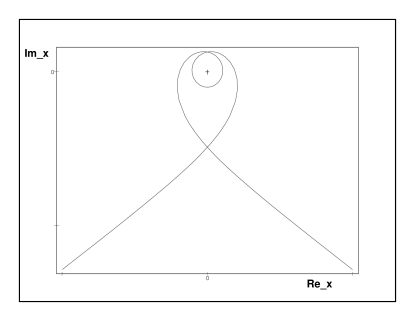
Figure 2: Sample of the curve ${\cal C}^{(N)}$ with $N=2$.

2 Integration paths ${\cal C}^{(N)}$

In certain complex domains of $r$, the general solution of any ordinary linear differential equation of the second order can be expressed as a superposition of some of its two linearly independent solutions,

$$\psi(r)=c_{1}\,\psi^{(1)}(r)+c_{2}\,\psi^{(2)}(r)\,.$$ (4)

In our present class of models (2) let us distinguish between the subdomains of the very small, intermediate and very large $|r|$. In the former case we can choose

$$\psi^{(1)}(r)=r^{\ell+1}+corrections\,,\ \ \ \ \psi^{(2)}(r)=r^{-\ell}+corrections\,,\ \ \ \ \ \ \ \ \ \ |r|\ll 1\,,$$ (5)

while we would prefer another option in the latter extreme, with $\kappa=\sqrt{E}$ in

$$\psi^{(1,2)}(r)=\exp\left({\pm{\rm i}\,\kappa\,r}\right)+corrections\,,\ \ \ \ \ \ \ |r|\gg 1\,.$$ (6)

In between these two regimes, our differential eq. (2) is smooth and analytic so that we may expect that all its solutions (4) are also locally analytic.

In the vicinity of the origin $r=0$ our differential equation has a pole. For the time being let us assume that our real parameter $\ell$ in eq. (2) is irrational. In such a case, both the components of our wave functions (4) (as well as their arbitrary superpositions) would behave, globally, as multivalued analytic functions defined on a certain multisheeted Riemann surface ${\cal R}$. In the other words, our wave functions possess a logarithmic branch point in the origin, i.e. a branch point with an infinite number of Riemann sheets connected at this point [9].

Separately, one might also study the simplified models with the rational $\ell$s which correspond to the presence of an algebraic branch point at $r=0$ which would connect a finite number of sheets [9]. Let us briefly mention here just the simplest possible scenario of such a type where $\ell(\ell+1)=0$ to that either $\ell=-1$ or $\ell=0$. In such a setting, eq. (4) just separates $\psi(r)$ into its even and odd parts so that the Riemann surface itself remains trivial, ${\cal R}\,\equiv\,l\!\!\!C$.

In the generic case of a multisheeted ${\cal R}$ we intend to show that the asymptotically free form of our differential eq. (2) with the independent solutions (6) can generate bound states. One must exclude, of course, the contours running, asymptotically, along the real line of $r$ since, in such a case, both our independent solutions $\psi^{(1,2)}(r)$ remain oscillatory and non-localizable. The same exclusion applies to the parallel, horizontal lines ${\cal C}^{(BG)}$ in the complex plane of $r$. In the search for bound states, both the “initial” and “final” asymptotic branches of our integration paths ${\cal C}^{(N)}$ must have the specific straight-line form $r=\pm|s|\,e^{{\rm i}\varphi}$ with a non-integer ratio $\varphi/\pi$. Thus, we may divide the asymptotic part of the complex Riemann surface of $r\in{\cal R}$ into the sequence of asymptotic sectors

$${\cal S}_{0}=\{r=-{\rm i}\,\varrho\,e^{{\rm i}\,\varphi}\,|\,\varrho\gg 1\,,\ \varphi\in(-\pi/2,\pi/2)\}\,.$$ (7)

$${\cal S}_{\pm k}=\{r=-{\rm i}\,e^{\pm{\rm i}\,k\,\pi}\,\varrho\,e^{{\rm i}\,\varphi}\,|\,\varrho\gg 1\,,\ \varphi\in(-\pi/2,\pi/2)\},\ \ \ \ k=1,2,\ldots\,.$$ (8)

We are now prepared to define the integration contours ${\cal C}^{(N)}$. For the sake of convenience, we shall set all their “left” asymptotic branches ${\cal C}^{(left)}$ in the same sector ${\cal S}_{0}$ and specify $r=\left(s+s_{0}\right)\,(1+{\rm i}\varepsilon)$ where $s\in(-\infty,-s_{0})$, $\varepsilon>0$ and $s_{0}>0$. The subsequent middle part of ${\cal C}^{(N)}$ must make $N$ counterclockwise rotations around the origin inside ${\cal R}$ while $s\in(-s_{0},s_{0})$. Finally, the “outcoming” or “right” asymptotic branch of our integration contour ${\cal C}^{(N)}$ with $s\in(s_{0},\infty)$ must lie in another sector ${\cal S}_{2N}$ of ${\cal R}$, i.e., in the Riemann sheet where the requirement of ${\cal PT}-$symmetry [7] forces us to set $r=\left(s-s_{0}\right)\,(1-{\rm i}\varepsilon)$. In this spirit, our illustrative Figures 1 – 3 sample the choice of $N=1$, $N=2$ and $N=3$, respectively.

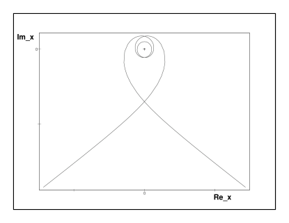
Figure 3: Sample of the curve ${\cal C}^{(N)}$ with $N=3$.

3 Bound states along nontrivial paths

It remains for us to impose the asymptotic boundary conditions requiring that our wave functions vanish at $s\to\pm\infty$. As long as our integration path ${\cal C}^{(N)}$ performs $N$ counterclockwise rotations around the origin, this form of the asymptotic boundary conditions will already guarantee the normalizability of our bound-state wave functions $\psi(r)\in{\it I\!\!\!L}^{2}\left({\cal C}^{(N)}\right)$ (cf. the similar situation encountered in the models with confining potentials [1, 6, 10]).

In the subsequent step we may set $z=\kappa r$ and $\psi(r)=\sqrt{z}\,\varphi(z)$ in our bound-state problem (2) with the (by assumption, real) $E=\kappa^{2}$. This reduces eq. (2) to the Bessel differential equation with the pair of the two well known independent special-function (say, Hankel-function [11]) solutions which may be inserted in our ansatz (9),

$$\psi(r)=c_{1}\,\sqrt{r}\,H^{(1)}_{\nu}(\kappa\,r)+c_{2}\,\sqrt{r}\,H^{(2)}_{\nu}(\kappa\,r)\,,\ \ \ \ \nu=\ell+1/2\,.$$ (9)

At $|{\rm arg}\,z|<\pi$ and ${\rm Re}\,\nu>-1/2$, the asymptotics of its components are given by the respective formulae 8.451.3 and 8.451.4 of ref. [11],

$$\sqrt{\frac{\pi z}{2}}\,H^{(1)}_{\nu}(z)=\exp\left[{\rm i}\left(z-\frac{\pi(2\nu+1)}{4}\right)\right]\,\left(1-\frac{\nu^{2}-1/4}{2{\rm i}z}+\ldots\right)\,,$$

$$\sqrt{\frac{\pi z}{2}}\,H^{(2)}_{\nu}(z)=\exp\left[-{\rm i}\left(z-\frac{\pi(2\nu+1)}{4}\right)\right]\,\left(1+\frac{\nu^{2}-1/4}{2{\rm i}z}+\ldots\right)\,.$$

This implies that inside the even-subscripted sectors ${\cal S}_{2k}$ our ansatz (9) combines the asymptotically growing (and, hence, unphysical) component $H^{(1)}_{\nu}(z)$ with the asymptotically vanishing and normalizable, physical component $H^{(2)}_{\nu}(z)$. Vice versa, in all the odd-subscripted sectors ${\cal S}_{2k+1}$ we would have to eliminate, in principle, the asymptotically growing $H^{(2)}_{\nu}(z)$ and to keep the asymptotically vanishing $H^{(1)}_{\nu}(z)$.

We may start our discussion of the existence of the localized bound states from the straight-line contour ${\cal C}={\cal C}^{(BG)}={\cal C}^{(0)}$ which is all contained in the zeroth sector ${\cal S}_{0}$. This immediately implies that with ${\rm Im}\,r\ll-1$, the asymptotically vanishing solution

$$\psi^{(1)}(r)=\sqrt{r}\,H^{(2)}_{\nu}(\kappa\,r)=const\,\cdot\,\exp(-{\rm i}\,\kappa\,r)+corrections\,$$

remains unconstrained at all the real $\kappa$. Obviously, the spectrum remains non-empty and bounded from below. This means that the low-lying states remain stable with respect to a random perturbation. A less usual feature of such a model is that its energies densely cover all the real half-line $I\!\!R^{+}$. This feature is fairly interesting per se, although a more detailed analysis of its possible physical consequences lies already beyond the scope of our present brief note.

Our eigenvalue problem becomes not too much more complicated when we turn attention to the spiral- or knot-shaped integration contours ${\cal C}^{(N)}$ with $N>0$. In such a case, fortunately, the exact solvability of our differential equation enables us to re-write ansatz (4) in its fully explicit form which remains analytic on all our Riemann surface ${\cal R}$. Once we choose our “left” asymptotic sector as ${\cal S}_{0}$, the “left” physical boundary condition fixes and determines the acceptable solution on the initial sheet,

$$\psi(r)=c\,\sqrt{r}\,H^{(2)}_{\nu}(\kappa r)\,,\ \ \ \ \ r\in{\cal S}_{0}\,.$$ (10)

After the $N$ counterclockwise turns of our integration path ${\cal C}^{(N)}$ around the origin this solution gets transformed in accordance with formula 8.476.7 of ref. [11] which plays a key role also in some other solvable models [12],

$$H^{(2)}_{\nu}\left(ze^{{\rm i}m\pi}\right)=\frac{\sin(1+m)\pi\nu}{\sin\pi\nu}\,H^{(2)}_{\nu}(z)+e^{{\rm i}\pi\nu}\,\frac{\sin m\pi\nu}{\sin\pi\nu}\,H^{(1)}_{\nu}(z)\,.$$ (11)

Here we have to set $m=2N$. This means that the existence of a bound state will be guaranteed whenever we satisfy the “right” physical boundary condition, i.e., whenever we satisfy the elementary requirement of the absence of the unphysical component $H^{(1)}_{\nu}(z)$ in the right-hand side of eq. (11).

The latter requirement is equivalent to the doublet of conditions

$$2N\nu=integer\,,\ \ \ \ \ \nu\neq integer\,.$$ (12)

This means that at any fixed and positive value of the energy $E=\kappa^{2}$ and at any fixed winding number $N=1,2,\ldots$, our present quantum-knot model generates the series of the bound states at certain irregular sequence of angular momenta avoiding some “forbidden” values,

$$\ell=\frac{M-N}{2N}\,,\ \ \ \ \ M=1,2,3,\ldots\,,\ \ \ \ \ M\neq 2N,4N,6N,\ldots\,.$$ (13)

These bound states exist and have the analytically continued Hankel-function form (10) if and only if the kinematical input represented by the angular momenta $\ell$ is restricted to the subset represented by formula (13).

Our construction is completed. Once we restrict our attention to the purely kinematic model with $\gamma=0$, we can summarize that at the odd dimensions $D=2p+1$ giving $\ell=n+p-3/2$ we may choose any index $n$ and verify that formula (13) can be read as a definition of the integer quantity $M=(2n+2p-1)\,N$ which is not forbidden. At the even dimensions $D=2p$ we equally easily verify that the resulting $M$ is always forbidden so that our quantum-knot bound states do not exist at $V(r)=0$ at all.

The latter dichotomy appears reminiscent of its well-known non-quantum real-space analogue, but the parallel is misleading because in quantum case the freedom of employing an additional coupling constant $\gamma$ enables us to circumvent the restrictions. Indeed, once we select any dimension $D$, angular-momentum index $m$, winding number $N$ and any “allowed” integer $M$, our spectral recipe (13) may simply be re-read as an explicit definition of the knot-supporting value of the coupling constant

$$\gamma=\left(\frac{M}{2N}\right)^{2}-\left(m+\frac{D-2}{2}\right)^{2}\,.$$

This implies that at non-vanishing $\gamma$s, the quantum knots can and do exist at all dimensions.

4 Discussion

4.1 Complexified coordinates

In the language of physics, our present construction and solution of a new and fairly unusual exactly solvable quantum model of bound states is based on the freedom of choosing the knot-shaped, complex contours of integration ${\cal C}$. This trick is not new [1, 4] and may be perceived as just a consequence of the admitted loss of the observability of the coordinates in PT-symmetric Quantum Mechanics [13].

From an experimentalist’s point of view, the omission of the standard assumption that the coordinate “should be” an observable quantity, $x\in I\!\!R$, is not entirely unacceptable since the current use of the concept of quasi-particles paved the way for similar constructions. Related Hamiltonians could be called, in certain sense, manifestly non-Hermitian. Still, they are currently finding applications in nuclear physics (where they are called quasi-Hermitian [14]). The loss of the reality of the coordinates is also quite common in field theory where the similar unusual Hamiltonians are being rather called CPT-symmetric [15] or crypto-Hermitian [16].

In a pragmatic phenomenological setting, the fairly unusual nature of the new structures of spectra seems promising. At the same time, the formalism itself is now considered fully consistent with the standard postulates of quantum theory. In the language of mathematics, the emergence of its innovative features may be understood as related to the non-locality in $x$, i.e., to the replacement of the standard scalar product

$$\langle\psi\,|\,\phi\rangle=\int\psi^{*}(x)\phi(x)dx$$

by its generalized, nonlocal modifications [13, 17]

$$\langle\psi\,|\,\phi\rangle=\int\psi^{*}(x)\,\Theta(x,y)\,\phi(y)dx\,dy\,.$$

Although this leaves an overall mathematical consistency and physical theoretical framework of Quantum Theory virtually unchanged [13], a new space is being open, inter alii, to the topology-based innovations. In principle, they might inspire new developments of some of the older successful applications of the formalism ranging from innovative supersymmetric constructions [18] to cosmology [19], occasionally even leaving the domain of quantum physics [20].

4.2 Towards a simplification of mathematics

The very existence of the present knot-type model is certainly based on nontrivial, non-Dirac scalar-product Hilbert-space kernels $\Theta\neq I$ (which is our present symbol for the quantity denoted as $T$ in ref. [14] or as $\eta_{+}$ in refs. [21] or as a factorized symbol ${\cal CP}$ in ref. [15] or ${\cal PQ}$ in [22] etc). This being said, a part of the price for an enhancement of the scope of the theory lies in the necessity of the explicit study of the equivalence transformations between the simple quantum model (which is non-Hermitian and ${\cal PT}-$symmetric) and its “physical”, Hermitian alternative representation(s) $H^{(Hermitian)}$. This transformation is not only non-local and complicated but also strongly Hamiltonian-dependent.

One could try to re-establish some parallels with the exceptional Buslaev’s and Grecchi’s oscillators [1] where $H^{(Hermitian)}$ happened to be, incidentally, still of a local, differential-equation nature. In the similar fortunate cases (cf. also ref. [23] for another illustration), the construction of $H^{(Hermitian)}$ remained reducible to the construction of a certain effective interaction $V^{(eff)}(r)\in I\!\!R$.

Partially, a similar technique of simplification can be also applied to our present model with $V=0$. Indeed, although it seems that all the variations of the spectrum must be attributed to the mere kinematical aspects of the model in question, one could employ the philosophy of ref. [6] to imagine that the nonequivalent effective interactions $V^{(eff)}(r)$ could be also attributed to the nonequivalent knot-shaped integration contours ${\cal C}^{(N)}$. An implementation of such a perspective would rely upon the conformal mapping

$$r=-{\rm i}\,e^{{\rm i}\,x/2}\,.$$ (14)

It simply maps each Riemann sheet in $r$ on a stripe in complex $x-$plane where $\Re e\ x$ plays the role of the angular coordinate while $\Im m\ x$ simulates the radial coordinate. In the other words, the polar-coordinates-resembling mapping (14) can be used to compress several sheets of a multisheeted Riemann surface ${\cal R}$ onto the single reference complex plane of the auxiliary complex variable $x$. In this manner an effective potential would emerge quite naturally (cf. also ref. [12] in this respect).

5 Outlook

We can summarize that our present example belongs to such a type of quantum theory where

• “coordinates” $r$ may complexify and lose their immediate observability,

• the topological structure of paths ${\cal C}$ can often be simplified via suitable conformal changes of variables [6, 7, 8],

• a “suitable” [14, 15, 21, 24] redefinition of the inner product in the Hilbert space is needed,

• complex potentials $V(r)\in l\!\!\!C$ are allowed.

Let us add, finally, a few remarks on the latter, nontrivial and appealing point. Firstly, one must imagine that our present, exactly solvable $N>1$ quantum-knot bound-state problem would become purely numerical after its immersion in virtually any external confining potential. Secondly, the survival of the reality of the new bound-state spectra (i.e., of the measurability of the energies) would have to be individually secured or proved as the necessary condition of the physical acceptability of the models with $V(r)\neq 0$.

The latter point has already been properly emphasized by Bender and Boettcher [4] who choose the one-parametric family of the one-dimensional power-law forces $V^{(BB)}(x)=x^{2}({\rm i}\,x)^{\delta}\,$ and supported the conjecture $E\in I\!\!R$ by the persuasive numerical and semiclassical arguments. The more rigorous (and unexpectedly difficult) proof only followed several years later [25]. It is worth noticing that the latter proof found also its most natural formulation in the general $D-$dimensional setting with $D>1$ and/or with the variable real $\ell$.

One of the merits of working with the power-law-dominated confining potentials was that the asymptotic behavior of the related wave functions can be analyzed easily (cf. also refs. [1, 4] and [10] where such an analysis has been performed and discussed in detail). One of the less expected results of these studies (revealed, tested and verified also by several other groups of authors [5, 12, 26] during 1998 - 1999) has been the observation of the explicit contour-dependence of the spectra. In fact, this discovery, so important in our present context, is even older since its first indications can even be traced back to the pioneering 1993 letter by Bender and Turbiner [27]. In our papers [6, 7] we emphasized and extended this observation by contemplating the “usual” potentials in combination with the “unusual”, topologically nontrivial, spiral-shaped contours ${\cal C}={\cal C}^{(N)}$ of complex coordinates.

On this background, the exact solvability of the present, force-free example came as a surprise. It could be perceived as an important new illustration of the changes of the energy spectra mediated by the use of the non-equivalent integration contours. Still, in the nearest future, a more numerically-oriented return to the more realistic problem of the contour-shape-dependence of the spectra generated by some nontrivial ${\cal PT}-$symmetric potentials in eq. (2) seems unavoidable.

Figure captions

Figure 1. Sample of the curve ${\cal C}^{(N)}$ with $N=1$.

Figure 2. Sample of the curve ${\cal C}^{(N)}$ with $N=2$.

Figure 3. Sample of the curve ${\cal C}^{(N)}$ with $N=3$.

References

- [1] V. Buslaev and V. Grecchi, J. Phys. A: Math. Gen. 26 (1993) 5541.
- [2] V. Grecchi, private communication
- [3] C. M. Bender and K. Milton, Phys. Rev. D 55 (1997) R3255.
- [4] C. M. Bender and S. Boettcher, Phys. Rev. Lett. 80 (1998) 5243
- [5] C. M. Bender, S. Boettcher and P. N. Meisinger, J. Math. Phys. 40 (1999) 2201.
- [6] M. Znojil, Phys. Lett. A 342 (2005) 36.
- [7] M. Znojil, J. Phys. A: Math. Gen. 39 (2006) 13325.
- [8] M. Znojil, Phys. Lett. A, to appear (arXiv:0708.0087v1 [quant-ph] 1 Aug 2007, doi:10.1016/j.physleta.2007.07.072).
- [9] see e.g. ”branch point” in http://eom.springer.de.
- [10] Y. Sibuya, Global Theory of Second Order Linear Differential Equation with Polynomial Coefficient, North Holland, Amsterdam, 1975; G. Alvarez, J. Phys. A: Math. Gen. 27 (1995) 4589.
- [11] I. S. Gradshteyn and I. M. Ryzhik, Tablicy integralov, summ, ryadov i proizvedenii, Nauka, Moscow, 1971.
- [12] F. Cannata, G. Junker and J. Trost, Phys. Lett. A 246 (1998) 219.
- [13] C. M. Bender, Rep. Prog. Phys., to appear (hep-th/0703096).
- [14] F. G. Scholtz, H. B. Geyer and F. J. W. Hahne, Ann. Phys. (NY) 213 (1992) 74.
- [15] C. M. Bender, D. C. Brody and H. F. Jones, Phys. Rev. Lett. 89 (2002) 0270401 (quant-ph/0208076).
- [16] A. V. Smilga, Cryptogauge symmetry and cryptoghosts for crypto-Hermitian Hamiltonians, arXiv:0706.4064.
- [17] J. Phys. A: Math. Gen. 39 (2006), Nr. 32 (dedicated special issue: H. Geyer, D. Heiss and M. Znojil, editors, pp. 9963 - 10261).
- [18] C. M. Bender and K. A. Milton, Phys. Rev. D 57 (1998) 3595; M. Znojil, F. Cannata, B. Bagchi and R. Roychoudhury, Phys. Lett. B 483 (2000) 284; A. Mostafazadeh, Nucl. Phys. B 640 (2002) 419; M. Znojil, J. Phys. A: Math. Gen. 35 (2002) 2341.
- [19] A. Mostafazadeh, Class. Quantum Grav. 20 (2003) 155.
- [20] U. Guenther, F. Stefani and M. Znojil, J. Math. Phys. 46 (2005) 063504.
- [21] A. Mostafazadeh, J. Math. Phys. 43 (2002) 205 (math-ph/0107001) and 2814 (math-ph/0110016).
- [22] M. Znojil, SIGMA 4 (2008) 001, (arXiv: 0710.4432v3 [math-ph]).
- [23] B. Bagchi, A. Banerjee, E. Caliceti, F. Cannata, H. B. Geyer, C. Quesne and M. Znojil, Int. J. Mod. Phys. A 20 (2005) 7107.
- [24] B. Bagchi, C. Quesne and M. Znojil, Mod. Phys. Letters A 16 (2001) 2047 (quant-ph/0108096); M. Znojil, J. Nonlin. Math. Phys. 9, suppl. 2 (2002) 122 (quant-ph/0103054); M. Znojil, Rend. Circ. Mat. Palermo, Serie II, Suppl. 72 (2004) 211 (math-ph/0104012).
- [25] P. Dorey, C. Dunning and R. Tateo, J. Phys. A: Math. Gen. 34 (2001) L391; P. Dorey, C. Dunning and R. Tateo, J. Phys. A: Math. Gen. 34 (2001) 5679; K. C. Shin, Commun. Math. Phys. 229 (2002) 543.
- [26] F. M. Fernández, R. Guardiola, J. Ros and M. Znojil, J. Phys. A: Math. Gen. 32 (1999) 3105.
- [27] C. M. Bender and A. V. Turbiner, Phys. Lett. A 173 (1993) 442.