The formation of Spiral Arms and Rings in Barred Galaxies

Abstract

We propose a theory to explain the formation of both spirals and rings in barred galaxies using a common dynamical framework. It is based on the orbital motion driven by the unstable equilibrium points of the rotating bar potential. Thus, spirals, rings and pseudo-rings are related to the invariant manifolds associated to the periodic orbits around these equilibrium points. We examine the parameter space of three barred galaxy models and discuss the formation of the different morphological structures according to the properties of the bar model. We also study the influence of the shape of the rotation curve in the outer parts, by making families of models with rising, flat or falling rotation curves in the outer parts. The differences between spiral and ringed structures arise from differences in the dynamical parameters of the host galaxies.

1 Introduction

Bars are a very common feature of disc galaxies. In a sample of $186$ spirals drawn from the Ohio State University Bright Spiral Galaxy Survey, Eskridge et al. ([2000]) find that $56\%$ of the galaxies in the near infrared are strongly barred, while an additional $6\%$ are weakly barred. A large fraction of barred galaxies show two clearly defined spiral arms (e.g. Elmegreen & Elmegreen [1982]), often departing from the end of the bar at nearly right angles. This is the case for instance in NGC 1300, NGC 1365 and NGC 7552. Deep exposures show that these arms wind around the bar structure and extend to large distances from the centre (see for instance Sandage & Bedke [1994]). Almost all researchers agree that spiral arms and rings are driven by the gravitational field of the galaxy (see Toomre [1977] and Athanassoula [1984], for reviews). In particular, spirals are believed to be density waves in a disc galaxy (Lindblad [1963]). Toomre ([1969]) found that the spiral waves propagate towards the principal Lindblad resonances of the galaxy, where they damp down, and thus concludes that long-lived spirals need some replenishment. There are essentially three different possibilities for a spiral wave to be replenished. First, it can be driven by a companion or satellite galaxy. A direct, relatively slow, and close passage of another galaxy can form trailing shapes (e.g. Toomre [1969]; Toomre & Toomre [1972]; Goldreich & Tremaine [1978], [1979]; Toomre [1981] and references therein). They can also be excited by the presence of a bar. Several studies have shown that a rotating bar or oval can drive spirals (e.g. Lindblad [1960]; Toomre [1969]; Sanders & Huntley [1976]; Schwarz [1979], [1981]; Huntley [1980]). The third alternative, proposed by Toomre ([1981]), is the swing amplification feedback cycle. This starts with a leading wave propagating from the centre towards corotation. In doing so, it unwinds and then winds in the trailing sense, while being very strongly amplified. This trailing wave will propagate towards the centre, while a further trailing wave is emitted at corotation and propagates outwards, where it is dissipated at the Outer Lindblad Resonance. The inwards propagating trailing wave, when reaching the centre will reflect into a leading spiral, which will propagate outwards towards corotation, thus closing the feedback cycle. Danby ([1965]) argued that orbits in the gravitational potential of a bar play an important role in the formation of arms. He noted that orbits departing from the vicinity of the equilibrium points located at the ends of the bar describe loci with the shape of spiral arms and can be responsible for the transport of stars from within to outside corotation, and vice versa. Unfortunately, he did not set his work in a rigorous theoretical context, so that it remained purely phenomenological. He also investigated whether orbits can be responsible for ring-like structures, but in this case, he did not consider orbits departing from the ends of the bar as he previously did when accounting for the spiral arms.

Strongly barred galaxies can also show prominent and spectacular rings or partial rings. The origin of such morphologies has been studied by Schwarz ([1981], [1984], [1985]), who followed the response of a gaseous disc galaxy to a bar perturbation. He proposed that ring-like patterns are associated to the principal orbital resonances, namely ILR, CR, and OLR. There are different types of outer rings. Buta ([1995]) classified them according to the relative orientation of the ring and bar major axes. If these two axes are perpendicular, the outer ring is classified as $R_{1}$. If the two axes are parallel, the outer ring is classified as $R_{2}$. Finally, if both types of rings are present in the galaxy, the outer ring is classified as $R_{1}R_{2}$.

In Romero-Gómez et al. ([2006, 2007]), we propose that rings and spiral arms are the result of the orbital motion driven by the invariant manifolds associated to periodic orbits around unstable equilibrium points. In Romero-Gómez et al. ([2006]), we fix a barred galaxy potential and we study the dynamics around the unstable equilibrium points. We give a detailed definition of the invariant manifold associated to a periodic orbit. For the model considered, the invariant manifolds delineate well the loci of an $rR_{1}$ ring structure. In Romero-Gómez et al. ([2007]), we construct families of models based on simple, yet realistic, barred galaxy potentials. In each family, we vary one of the free parameters of the potential and keep the remaining fixed. For each model, we numerically compute the orbital structure associated to the invariant manifolds. In this way, we are able to study the influence of each model parameter on the global morphologies delineated by the invariant manifolds.

In Sect. 2, we first present the equations of motion and the galactic models used in the computations. In Sect. 3, we give a brief description of the dynamics around the unstable equilibrium points. In Sect. 4, we show the different morphologies that result from the computations. In Sect. 5, we compare our results with some observational features and conclude.

2 Equations of motion and description of the model

We model the potential of a barred galaxy as the superposition of three components, two of them axisymmetric and the third bar-like. The last component rotates anti-clockwise with angular velocity ${\bf\Omega_{p}}=\Omega_{p}{\bf z}$, where $\Omega_{p}$ is a constant pattern speed  . The equations of motion in this potential in a frame rotating with angular speed ${\bf\Omega_{p}}$ in vector form are

$${\bf\ddot{r}=-\nabla\Phi}-2{\bf(\Omega_{p}\times\dot{r})-\Omega_{p}\times(\Omega_{p}\times r)},$$ (1)

where the terms $-2{\bf\Omega_{p}\times\dot{r}}$ and $-{\bf\Omega_{p}\times(\Omega_{p}\times r)}$ represent the Coriolis and the centrifugal forces, respectively, and ${\bf r}$ is the position vector. We define an effective potential $\Phi_{\hbox{\scriptsize eff}}=\Phi-\frac{1}{2}\Omega_{p}^{2}\,(x^{2}+y^{2}),$ then Eq. (1) becomes ${\bf\ddot{r}=-\nabla\Phi_{\hbox{\scriptsize eff}}}-2{\bf(\Omega_{p}\times\dot{r})},$ and the Jacobi constant is

$$E_{J}=\frac{1}{2}{\bf\mid\dot{r}\mid}^{2}+\Phi_{\hbox{\scriptsize eff}},$$ (2)

which, being constant in time, can be considered as the energy in the rotating frame.

The axisymmetric component consists of the superposition of a disc and a spheroid. The disc is modelled as a Kuzmin-Toomre disc (Kuzmin [1956]; Toomre [1963]) of surface density $\sigma(r)$ and the spheroid is modelled using a density distribution of the form $\rho(r)$:

$$\sigma(r)=\frac{V_{d}^{2}}{2\pi r_{d}}\left(1+\frac{r^{2}}{r_{d}^{2}}\right)^{-3/2},\qquad\rho(r)=\rho_{b}\left(1+\frac{r^{2}}{r_{b}^{2}}\right)^{-3/2}.$$ (3)

The parameters $V_{d}$ and $r_{d}$ set the scales of the velocities and radii of the disc, respectively, and $\rho_{b}$ and $r_{b}$ determine the concentration and scale-length of the spheroid. In our models, we use three bar potentials to compare the results obtained. The first bar potential is described by a Ferrers ([1877]) ellipsoid whose density distribution is:

$$\left\{\begin{array}[]{lr}\rho_{0}(1-m^{2})^{n}&m\leq 1\\ 0&m\geq 1,\end{array}\right.$$ (4)

where $m^{2}=x^{2}/a^{2}+y^{2}/b^{2}$. The values of $a$ and $b$ determine the shape of the bar, $a$ being the length of the semi-major axis, which is placed along the $x$ coordinate axis, and $b$ being the length of the semi-minor axis. The parameter $n$ measures the degree of concentration of the bar and $\rho_{0}$ represents the bar central density. We also use two ad-hoc potentials, namely a Dehnen’s bar type, $\Phi_{1}$, (Dehnen [2000]) and a Barbanis-Woltjer (BW) bar type, $\Phi_{2}$, (Barbanis & Woltjer [1967]):

$$\Phi_{1}(r,\theta)=-\frac{1}{2}\epsilon v_{0}^{2}\cos(2\theta)\left\{{\begin{array}[]{ll}\displaystyle 2-\left(\frac{r}{\alpha}\right)^{n},&r\leq\alpha\rule[-14.22636pt]{0.0pt}{28.45274pt}\\ \displaystyle\left(\frac{\alpha}{r}\right)^{n},&r\geq\alpha.\rule[-14.22636pt]{0.0pt}{28.45274pt}\end{array}}\right.\qquad\Phi_{2}(r,\theta)=\hat{\epsilon}\sqrt{r}(r_{1}-r)\cos(2\theta)$$ (5)

The parameter $\alpha$ is a characteristic length scale of the Dehnen’s type bar potential, and $v_{0}$ is a characteristic circular velocity. The parameter $\epsilon$ is related to the bar strength. The parameter $r_{1}$ is a characteristic scale length of the BW bar potential and the parameter $\hat{\epsilon}$ is related to the bar strength.

3 Dynamics around the $L_{1}$ and $L_{2}$ equilibrium points

For our calculations we place ourselves in a frame of reference corotating with the bar, and the bar semi-major axis is located along the $x$ axis. In this rotating frame we have five equilibrium Lagrangian points (see left panel of Fig. 1). Three of these points are stable, namely $L_{3}$, which is placed at the centre of the system, and $L_{4}$ and $L_{5}$, which are located symmetrically on the $y$ axis. $L_{1}$ and $L_{2}$ are unstable and are located symmetrically on the $x$ axis. The surface $\Phi_{\hbox{\scriptsize eff}}=E_{J}$ ($E_{J}$ defined as in Eq. (2)) is called the zero velocity surface, and its intersection with the $z=0$ plane gives the zero velocity curve. All regions in which $\Phi_{\hbox{\scriptsize eff}}>E_{J}$ are forbidden to a star with this energy, and are thus called forbidden regions. The zero velocity curve also defines two different regions, namely, an exterior region and an interior one that contains the bar. The interior and exterior regions are connected via the equilibrium points (see middle panel of Fig. 1). Around the equilibrium points there exist families of periodic orbits, e.g. around the central equilibrium point the well-known $x_{1}$ family of periodic orbits that is responsible for the bar structure.

The dynamics around the unstable equilibrium points is described in detail in Romero-Gómez et al. ([2006]), here we give a brief summary. Around each unstable equilibrium point there also exists a family of periodic orbits, known as the family of Lyapunov orbits (Lyapunov [1949]). For a given energy level, two stable and two unstable sets of asymptotic orbits emanate from the periodic orbit, and they are known as the stable and unstable invariant manifolds, respectively. We denote by $W^{s}_{\gamma_{i}}$ the stable invariant manifold associated to the periodic orbit $\gamma$ around the equilibrium point $L_{i},\,i=1,2$. This stable invariant manifold is the set of orbits that tends to the periodic orbit asymptotically. In the same way we denote by $W^{u}_{\gamma_{i}}$ the unstable invariant manifold associated to the periodic orbit $\gamma$ around the equilibrium point $L_{i},\,i=1,2$. This unstable invariant manifold is the set of orbits that departs asymptotically from the periodic orbit (i.e. orbits that tend to the Lyapunov orbits when the time tends to minus infinity), see right panel of Fig. 1. Since the invariant manifolds extend well beyond the neighbourhood of the equilibrium points, they can be responsible for global structures.

In Romero-Gómez et al. ([2007]), we give a detailed description of the role invariant manifolds play in global structures, in particular, in the transfer of matter. Simply speaking, the transfer of matter is characterised by the presence of homoclinic, heteroclinic, and transit orbits.

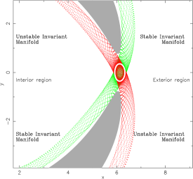
Figure 1: Dynamics around the $L_{1}$ and $L_{2}$ equilibrium points. Left panel: location of the equilibrium points and outline of the bar. Middle panel: Zero velocity curves and Lyapunov orbits around $L_{1}$ and $L_{2}$. Right panel: Stable, $W^{s}_{\gamma_{1}}$ in green, and unstable, $W^{u}_{\gamma_{1}}$ in red, invariant manifolds of a periodic orbit around $L_{1}$.

Homoclinic orbits correspond to asymptotic trajectories, $\psi$, such that $\psi\in W^{u}_{\gamma_{i}}\cap W^{s}_{\gamma_{i}},\,i=1,2$. Thus, a homoclinic orbit departs asymptotically from the unstable Lyapunov periodic orbit $\gamma$ around $L_{i}$ and returns asymptotically to it (see Fig. 2a). Heteroclinic orbits are asymptotic trajectories, $\psi^{\prime}$, such that $\psi^{\prime}\in W^{u}_{\gamma_{i}}\cap W^{s}_{\gamma_{j}},\,i\neq j,\,i,j=1,2$. Thus, a heteroclinic orbit departs asymptotically from the periodic orbit $\gamma$ around $L_{i}$ and asymptotically approaches the corresponding Lyapunov periodic orbit with the same energy around the Lagrangian point at the opposite end of the bar $L_{j}$, $i\neq j$ (see Fig. 2b). There also exist trajectories that spiral out from the region of the unstable periodic orbit, and we refer to them as transit orbits (see Fig. 2c).

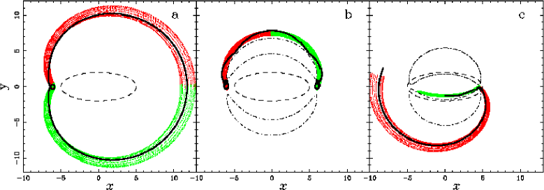
Figure 2: Homoclinic (a), heteroclinic (b) and escaping (c) orbits (black thick lines) in the configuration space. In red lines, we plot the unstable invariant manifolds associated to the periodic orbits, while in green we plot the corresponding stable invariant manifolds. In dashed lines, we give the outline of the bar and, in (b) and (c), we plot the zero velocity curves in dot-dashed lines.

4 Results

Here we describe the main results obtained when we vary the parameters of the models introduced in Sect. 2. In order to best see the influence of each parameter separately, we make families of models in which only one of the free parameters is varied, while the others are kept fixed. Our results in Romero-Gómez et al. ([2007]) show that only the bar pattern speed and the bar strength have an influence on the shape of the invariant manifolds, and thus, on the morphology of the galaxy. We have also studied the influence of the shape of the rotation curve. We make models with either rising, flat or falling rotation curve in the outer parts.

Our results also show that the morphologies obtained do not depend on the bar potential we use, but on the presence of homoclinic or heteroclinic orbits. Thus, if the model does not have either heteroclinic nor homoclinic orbits and only transit orbits are present, the barred galaxy will present two spiral arms emanating from the ends of the bar. The outer branches of the unstable invariant manifolds will spiral out from the ends of the bar and they will not return to its vicinity. If the transit orbits associated to the $W^{u}_{\gamma_{1}}$ intersect in configuration space with the transit orbits associated to $W^{u}_{\gamma_{2}}$, then they form the characteristic shape of $R_{2}$ rings. That is, the trajectories outline an outer ring whose principal axis is parallel to the bar major axis. If heteroclinic orbits exist, then the ring of the galaxy is classified as $rR_{1}$. The inner branches of the invariant manifolds associated to $\gamma_{1}$ and $\gamma_{2}$ outline a nearly circular inner ring that encircles the bar. The outer branches of the same invariant manifolds form an outer ring whose principal axis is perpendicular to the bar major axis. The last possibility is if only homoclinic orbits exist. In this case, the inner branches of the invariant manifolds for an inner ring, while the outer branches outline both types of outer rings, thus the barred galaxy presents an $R_{1}R_{2}$ ring morphology.

5 Discussion

The family of Lyapunov orbits is unstable and becomes stable only at high energy levels (Skokos et al. ([2002]). We compute the invariant manifolds of Lyapunov orbits in the range of energies in which they are unstable. In the right panel of Fig. 3, we plot the invariant manifolds for two different energy levels of a given model. We find that the locus of the invariant manifolds is independent of the energy. As the energy increases, however, the size of the Lyapunov orbits also increases and thus the size of the invariant manifolds. Nevertheless, as we consider more energy levels, we find that the density in the central part is higher (see left panel of Fig. 3). Therefore, the thickness of the ring observed is smaller than the thickness of the invariant manifold of higher energies. We also compute the radial and tangential velocities on the galactic plane and in a non-rotating reference frame along the ring and we observe that they are small perturbations of the circular velocity. The maximum deviation from the typical circular velocity of $200\rm{km}\,\rm{s}^{-1}$ is $\pm 20\rm{km}\,\rm{s}^{-1}$ (Athanassoula et al. [2007]).

In the case of the spiral arms, we compute the density profile on two different angles, namely one near the beginning of the arm and one at the end. We find that the first cut has a narrow and high density profile, while the second cut, has a wide and low density profile. This is the typical behaviour of the grand design spiral arms, namely they are denser and brighter near the bar ends and then they become more diffuse (Athanassoula et al. [2007]).

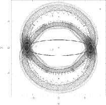
Figure 3: Left panel: Density profile on a cut across the ring. Right panel: Two unstable invariant manifolds for different values of $E_{J}$. Note how similar the regions they delineate are.

To summarise, our results show that invariant manifolds describe well the loci of the different types of rings and spiral arms. They are formed by a bundle of trajectories linked to the unstable regions around the $L_{1}/L_{2}$ equilibrium points. The study of the influence of one model parameter on the shape of the invariant manifolds in the outer parts reveals that only the pattern speed and the bar strength affect the galaxy morphology. The study also shows that the different ring types and spirals are obtained when we vary the model parameters.

We have compared our results with some observational data. Regarding the photometry, the density profiles across radial cuts in rings and spiral arms agree with the ones obtained from observations. The velocities along the ring also show that these are only a small perturbation of the circular velocity.