Properties of contact matrices induced by pairwise interactions in proteins

Abstract

The properties of contact matrices ($C$ matrices) needed for native proteins to be the lowest-energy conformations are considered in relation to a contact energy matrix ($E$ matrix). The total conformational energy is assumed to consist of pairwise interaction energies between atoms or residues, each of which is expressed as a product of a conformation-dependent function (an element of the $C$ matrix) and a sequence-dependent energy parameter (an element of the $E$ matrix). Such pairwise interactions in proteins force native $C$ matrices to be in a relationship as if the interactions are a Go-like potential [N. Go, Annu. Rev. Biophys. Bioeng. 12. 183 (1983)] for the native $C$ matrix, because the lowest bound of the total energy function is equal to the total energy of the native conformation interacting in a Go-like pairwise potential. This relationship between $C$ and $E$ matrices corresponds to (a) a parallel relationship between the eigenvectors of the $C$ and $E$ matrices and a linear relationship between their eigenvalues, and (b) a parallel relationship between a contact number vector and the principal eigenvectors of the $C$ and $E$ matrices, where the $E$ matrix is expanded in a series of eigenspaces with an additional constant term. The additional constant term in the spectral expansion of the $E$ matrix is indicated by the lowest bound of the total energy function to correspond to a threshold of contact energy that approximately separates native contacts from non-native ones. Inner products between the principal eigenvector of the $C$ matrix, that of the $E$ matrix, and a contact number vector have been examined for 182 proteins each of which is a representative from each family of the SCOP database [A. G. Murzin et al., J. Mol. Biol. 247, 536 (1995)], and the results indicate the parallel tendencies between those vectors. A statistical contact potential [S. Miyazawa and R. L. Jernigan, Proteins 34, 49 (1999); 50, 35 (2003)] estimated from protein crystal structures was used to evaluate pairwise residue-residue interactions in the proteins. In addition, the spectral representation of $C$ and $E$ matrices reveals that pairwise residue-residue interactions, which depends only on the types of interacting amino acids but not on other residues in a protein, are insufficient and other interactions including residue connectivities and steric hindrance are needed to make native structures the unique lowest-energy conformations.

I Introduction

Predicting a protein three dimensional structure from its sequence is equivalent to reproducing a three dimensional structure from one dimensional information encoded in its sequence. From such a viewpoint, there are many studies that try to reconstruct three dimensional structures from one dimensional information such as contact numbers and the principal eigenvector of a contact matrix KKVD:02 ; PBRV:04 ; KN:05 ; VWP:06 . An important question is not only what kind of one dimensional information is needed to reconstruct protein structures but also why such information is critical to reconstruct protein structures.

Let us think about a distance matrix each element of which is equal to distance between atoms or residues specified by its column and row. Information contained in the distance matrix is equivalent with the specification of three-dimensional coordinates of each atom or residue, except that a mirror image of the native structure cannot be excluded in distance information. Reconstructing a distance matrix from one-dimensional vectors requires in principle the specification of all eigenvectors as well as eigenvalues. In other words, for an $N\times N$ matrix, $N$ $N$-dimensional vectors are required. However, protein’s particular characteristics may allow the reconstruction of a distance matrix with fewer one-dimensional vectors.

A contact matrix whose element is equal to one for contacting atom or residue pairs or zero for no-contacting atom or residue pairs on the basis of distance between the two atoms/residues, is a simplification of a distance matrix with two categories, contact or non-contact, but keeps almost all information needed to reconstruct three-dimensional structures of proteins. In the case of a residue-residue contact matrix consisting of discrete values, one and zero, Porto et al. PBRV:04 showed that the contact map of the native structure of globular proteins can be reconstructed starting from the sole knowledge of the contact map’s principal eigenvector, and the reconstructed contact map allow in turn for an accurate reconstruction of the three-dimensional structure.

A vector of contact numbers, which is defined as the number of atoms or residues in contact with each atom or residue in a protein, is another type of one-dimensional vector that is often used as a one-dimensional representation of protein structures NO:80 ; NO:86 ; KHN:05 , and may be similar to but not the same as the principal eigenvector of a contact matrix. Kabakçioǧlu et al. KKVD:02 suggested that the number of feasible protein conformations that satisfy the constraint of a contact number for each residue is very limited.

A question is why the principal eigenvector of a contact matrix and a contact number vector contain significant information on protein structures. Here, we consider what properties of contact matrices are induced by pairwise contact interactions for native proteins to be the lowest-energy conformations. For simplicity, a total conformational energy is assumed to consist of pairwise interactions over all atom or residue pairs. It is further assumed that the pairwise interaction can be expressed as a product of a conformation-dependent ($C$-dependent) factor and a sequence-dependent ($S$-dependent) factor. The $C$-dependent factor represents the degree of contact between atoms/residues and can be assumed without loss of generality to take any value between 0 and 1. The $S$-dependent factor corresponds to an energy parameter specific to a given pair of atoms or residues. Here we call a matrix of the $C$-dependent factor a generalized contact matrix or even simply a contact matrix ($C$ matrix), and call a matrix of the $S$-dependent factor a generalized contact energy matrix or even simply a contact energy matrix ($E$ matrix). A simple linear algebra indicates that such a total energy function is bounded by the lowest value corresponding to the total energy for a $C$ matrix in which all pairs with lower contact energies than a certain threshold are in contact. Such a lower bound is achieved KM:08 if and only if proteins are ideal to have the so-called Go-like potential G:83 . The Go-like potential is defined as the one in which interaction energies between native contacts are always lower than those between non-native contacts. Real pairwise interactions in proteins could not be the Go-like potential. In other words, real proteins could not achieve this lowest bound of a pairwise potential because of atom and residue connectivities and steric hindrance that are not included in this type of total energy function. How should they approach to the lowest bound as closely as possible? The lowest bound can be approached by making the singular vectors of the $C$ matrix parallel to the corresponding singular vectors of the $E$ matrix with the same value of the singular values. Also, in the lowest bound a contact number vector tends to be parallel to the principal eigenvectors of the $C$ and $E$ matrices. The most effective way would be to first make the principal singular vector of the $C$ matrix parallel to that of the $E$ matrix. A similar strategy was used to recognize protein structures by three-dimensional threading of protein sequences CIWMSDH:04 ; CWDIH:06 . Bastolla et al. BPRV:05 pointed out that the principal eigenvector of a contact matrix must be correlated with that of a contact energy matrix, if the free energy of a conformation folded into a contact map is approximated by a pairwise contact potential. It was shown that the correlation coefficients of these two principal eigenvectors are actually statistically significant in protein folds. However, unlike their analyses the lowest bound of the total energy indicates the $E$ matrix to be singular-decomposed with a constant term that corresponds to the threshold energy to separate native contacts from non-native ones. The eigenvectors of $E$ matrix depend on the value of the additional constant.

Based on the indication above, we have analyzed the relationships between the principal eigenvectors of the $C$ and $E$ matrices and contact number vector by examining the inner product of the two vectors. A statistical contact potential MJ:99 ; MJ:03 estimated from protein crystal structures is used to evaluate pairwise residue-residue interactions in proteins. One hundred and eighty-two representatives of single domain proteins from each family in the SCOP version 1.69 database MBHC:95 are used to analyze the relationship between the principal eigenvectors of the native $C$ and $E$ matrices and the contact number vector. Results show that the inner product of both the principal eigenvectors has a maximum at a certain value of the threshold energy for contacts, and that there are parallel tendencies between both the principal eigenvectors and contact number vector. It is worth noting that the principal eigenvector of the native $C$-matrix corresponds to the lower frequency normal modes of the native structure of protein.

In addition, the spectral representation of $C$ and $E$ matrices reveals that pairwise residue-residue interactions, which depend only on the types of interacting amino acids but not on other residues in a protein, are insufficient and other interactions including residue connectivities and steric hindrance are needed to make native structures unique lowest-energy conformations.

II Methods

Basic assumptions and conventions

We first assume that the total conformational energy of a protein with conformation $C$ and amino acid sequence $S$ of $N$ units can be approximated as the sum of pairwise interaction energies between the units. Here a single unit may consist of an atom or a residue, although in most cases we treat a residue as a unit. We further assume that each pairwise interaction term can be expressed as a product of a $C$-dependent factor and an $S$-dependent factor. The $C$-dependent factor represents the degree to which a pair of units are in contact, while the $S$-dependent factor represents an interaction energy for a contacting pair of units. In other words, the total conformational energy is assumed to be approximated as

$$E^{{\mbox{\scriptsize c}}}(C,S) = \frac{1}{2}\sum_{i}^{N}\sum_{j}^{N}\mathcal{E}_{ij}(S)\Delta_{ij}(C)$$ (1)

$$= \frac{1}{2}\sum_{i}^{N}\sum_{j}^{N}\delta\mathcal{E}_{ij}(S)\Delta_{ij}(C)+\varepsilon_{0}N_{{\mbox{\scriptsize c}}}(C){,}$$ (2)

$$\delta\mathcal{E}_{ij}(S) \equiv \mathcal{E}_{ij}(S)-\varepsilon_{0}{.}$$ (3)

where $\mathcal{E}_{ij}(S)$ and $\Delta_{ij}(C)$ are the $S$-dependent and $C$-dependent factors for the pairwise interaction energy between the $i$th and $j$th units, respectively. $N_{{\mbox{\scriptsize c}}}(C)$ is the total number of contacts between units and defined as

$$N_{{\mbox{\scriptsize c}}}(C) \equiv \frac{1}{2}\sum_{i}\sum_{j}\Delta_{ij}(C)=\frac{1}{2}\sum_{i}n_{i}(C){,}$$ (4)

where the generalized contact number $n_{i}$, which is the total number of units contacting with the $i$th unit, is defined as

$$n_{i}(C) = \sum_{j}^{N}\Delta_{ij}(C){.}$$ (5)

In Eq. (2), a constant $\varepsilon_{0}$ defined by Eq. (3) is introduced to explicitly treat the total number of contacts in the evaluation of the total energy.

Each $\Delta_{ij}(C)$ is a function of coordinates of the $i$th and $j$th units, and is assumed without loss of generality to take any value between 0 and 1, with the diagonal elements always defined to be equal to 0. The $S$-dependent term $\mathcal{E}_{ij}(S)$ can include not only two-body interactions but multi-body effects such as a mean-field, that is, it can not only depend on the type of a unit pair but on the entire protein sequence. We call the matrix $\Delta(C)\equiv(\Delta_{ij}(C))$ as a generalized contact matrix or $C$-matrix for short. Similarly, we call the matrix $(\mathcal{E}_{ij}(S))$ as a generalized contact energy matrix or $E$-matrix for short. Each element of the energy function of Eq. (1) can represent either attractive or repulsive interactions but not both. In the next sections, we consider the mathematical lower limits of the total contact energy, ignoring atomic details of proteins such as atom and residue connectivities and steric hindrance. The volume exclusions between atoms are assumed to be satisfied and are not included in the total energy function. To minimally reflect the effects of steric hindrance, the total number of contacts $N_{{\mbox{\scriptsize c}}}$ is explicitly treated in the evaluation of the total energy, Eq. (2), by introducing a constant $\varepsilon_{0}$. The expression for Eq. (1) can be regarded as a special case of Eq. (2) in which $\varepsilon_{0}$ is equal to zero.

Lower bounds of the total contact energy

Let us consider lower bounds of the total contact energy represented by Eq. (1) under a condition that each element of $C$-matrix can independently take any value within $0\leq\Delta_{ij}\leq 1$ irrespective of whether or not they can be reached in real protein conformations; in other words, atom and residue connectivities and steric hindrance are completely ignored.

If one regards $\delta\mathcal{E}_{ij}$ and $\Delta_{ij}$ as the elements of the vectors $\delta\vec{\mathcal{E}}(S)$ and $\vec{\Delta}(C)$ in $N^{2}$-dimensional Euclidean space, it will be obvious that the first term of Eq. (2) can be bounded by a product of the norms of those two vectors:

$$E^{{\mbox{\scriptsize c}}}(C,S) \geq \!\min_{\varepsilon_{0}}\,[\,-\,\frac{1}{2}\|\delta\vec{\mathcal{E}}(S)\|\|\vec{\Delta}(C)\|+\varepsilon_{0}N_{{\mbox{\scriptsize c}}}(C)\,]{,}$$ (6)

where $\|\ldots\|$ means a Euclidian norm. Obviously the equality of Eq. (6) is achieved if and only if those vectors are anti-parallel to each other:

$$\delta\mathcal{E}_{ij}(S) = \varepsilon\Delta_{ij}(C){,}$$ (7)

where $\varepsilon$ is a negative constant.

In addition, there is a simple mathematical limit for the total energy of Eq. (1) for which the $C$ matrix is equal to $H_{0}(-\delta\mathcal{E}_{ij})$:

$$E^{{\mbox{\scriptsize c}}}(C,S)$$ (8)

$$\geq \!\frac{1}{2}\sum_{i}\sum_{j}\delta\mathcal{E}_{ij}(S)\Delta_{ij}(C_{{\mbox{\scriptsize min}}})+\varepsilon_{0}(C_{{\mbox{\scriptsize min}}})N_{{\mbox{\scriptsize c}}}(C_{{\mbox{\scriptsize min}}})$$

$$\geq \!\frac{1}{2}\sum_{i}\sum_{j}\mathcal{E}_{ij}(S)H_{0}(-\mathcal{E}_{ij}(S)){,}$$ (9)

$$\Delta_{ij}(C_{{\mbox{\scriptsize min}}})=H_{0}(-\delta\mathcal{E}_{ij}(S)){,}$$ (10)

where $H_{0}(x)$ is the Heaviside step function that takes 1 for $x>0$ and 0 for otherwise. $C_{{\mbox{\scriptsize min}}}$ is the lowest-energy conformation with a constraint on the total contact number $N_{{\mbox{\scriptsize c}}}$, although it is not necessarily reached due to atom and residue connectivities, and steric hindrance. If each $\Delta_{ij}$ is allowed to take either 0 or 1 only, and also each $\delta\varepsilon_{ij}$ takes either one of two real values only to be able to satisfy Eq. (7), both the lower bounds of Eqs. (6) and 8 are equal to each other. Otherwise, the lower bound of Eq. (6) is further bounded by the lower bound of Eq. (8), or the equality in Eq. (6) cannot be achieved with $0\leq\Delta_{ij}\leq 1$, but Eq. (8) is always satisfied. If the total number of contacts $N_{{\mbox{\scriptsize c}}}$ is constrained to be equal to $N_{{\mbox{\scriptsize c}}}(C_{{\mbox{\scriptsize min}}})$, then $\varepsilon_{0}$ must be properly chosen as a non-positive value so that Eq. (4) is satisfied with $C=C_{{\mbox{\scriptsize min}}}$. Otherwise, $\varepsilon_{0}$ should be taken to be equal to 0 to obtain the lower bound of Eq. (9). Eq. (9) describes the lowest bound without any constraint on the number of contacts and corresponds to the energy of the conformation $C_{{\mbox{\scriptsize min}}}$ for the case of $\varepsilon_{0}=0$.

The potentials that satisfy Eq. (7) or 10 are just Go-like potentials G:83 , in which interactions between native contact pairs are always more attractive than those between non-native pairs. Let us call proteins with a Go-like potential as ideal proteins. There are multiple levels of nativelikeliness in the Go-like potential. The most nativelike potential of the present Go-like potentials is the one in which all interactions between native contacts are attractive and other interactions are all repulsive. In other words, $\mathcal{E}_{ij}$ is negative for native contacts and positive for non-native contacts. In such a Go-like potential, the native conformation can attain the lowest bound of Eq. (9), which is equivalent to Eq. (8) with $\varepsilon_{0}=0$. A less nativelike potential is the one in which interactions between non-native contact pairs can be attractive but always less attractive than those between native contact pairs. An ideal protein with such a potential can attain Eq. (8) with a proper value of $\varepsilon_{0}$, which is the threshold energy for native and non-native contacts. For real protein, we should define $\varepsilon_{0}$ as a threshold of contact energy under which unit pairs tend to be in contact in native conformations.

In ideal proteins, the lowest-energy conformation must be the one for which the contact potential looks like a Go-like potential, and inversely the potential must be a Go-like potential for the lowest-energy conformation. In real proteins, it would be impossible that contact potentials for native structures are exactly like a Go-like potential of Eq. (7) or Eq. (10), even though the contact potential being considered here may be the effective one that includes not only actual pairwise interactions but also the effects of higher order interactions near native structures. In other words, the lowest bound of Eq. (8) could not be achieved for real pairwise potentials, because of atom and residue connectivities and steric hindrance. However, it is desirable to reduce frustrations among interactions so that an effective pairwise potential in native structures must approach the Go-like potential. Then, a question is how native contact energies approach the mathematical lowest limit. In the following, we will give tips as to how the $C$-matrix should be designed to decrease the total energy towards the theoretical lowest limit.

It should be noted here that the lowest-energy conformation, the $C$ matrix, is considered for a given potential, the $E$ matrix, but not its inverse problem, which is to consider an optimum potential or an optimum sequence for a given conformation — that is, an optimum $E$ matrix for a given $C$ matrix. In the inverse problem, the total partition function varies depending on each sequence, and it must be taken into account to evaluate the stability of the given $C$ matrix in relative to the other conformations SVMB:96 ; DK:96 ; MoS:96 ; MJ:99a . The $Z$ score of the energy gap between the given $C$ matrix and other compact conformations may be used to evaluate the optimality of each sequence MAS:96 ; BPRV:05 .

Spectral relationship between $C$ and $E$ matrices

We apply singular value decomposition to both the $C$ matrix (generalized contact matrix) and $E$ matrix (generalized contact energy matrix). The $C$ matrix is decomposed as

$$\Delta_{ij}(C) = \sum_{\mu}|\lambda_{\mu}(C)|L_{i\mu}(C)R_{j\mu}(C){,}$$ (11)

$$|\lambda_{1}(C)| \geq \ldots\geq|\lambda_{N}(C)|\geq 0{,}$$ (12)

where $\lambda_{\mu}(C)$ is the eigenvalue of $\Delta(C)$, and its absolute value $|\lambda_{\mu}(C)|$ is the $\mu$th non-negative singular value of $\Delta(C)$ arranged in decreasing order, and ${\bf L}_{\mu}(C)\equiv\ ^{t}(L_{1\mu},\ldots,L_{N\mu})$ and ${\bf R}_{\mu}(C)\equiv\ ^{t}(R_{1\mu},\ldots,R_{N\mu})$ are the corresponding left and right singular vectors; both $L\equiv({\bf L}_{1},\ldots,{\bf L}_{N})$ and $R\equiv({\bf R}_{1},\ldots,{\bf R}_{N})$ are orthonormal matrices. Note that the singular values for a symmetric matrix such as a contact matrix are equal to the absolute value of its eigenvalue. We choose the eigenvector corresponding to the eigenvalue $\lambda_{\mu}(C)$ as a right singular vector ${\bf R}_{\mu}(C)$ and if $\lambda_{\mu}(C)\geq 0$, ${\bf L}_{\mu}(C)\equiv{\bf R}_{\mu}(C)$ and otherwise ${\bf L}_{\mu}(C)\equiv-\;{\bf R}_{\mu}(C)$.

Likewise, the $E$ matrix, $(\mathcal{E}_{ij}(S))$, is decomposed as

$$\mathcal{E}_{ij}(S) = \sum_{\nu}|\varepsilon_{\nu}|U_{i\nu}(S)V_{j\nu}(S)+\varepsilon_{0}{,}$$ (13)

$$|\varepsilon_{1}| \geq \ldots\geq|\varepsilon_{N}|\geq 0{,}$$ (14)

where the absolute value of the eigenvalue, $|\varepsilon_{\nu}(S)|$, ${\bf U}_{\nu}(S)\equiv\ ^{t}(U_{1\nu},\ldots,U_{N\nu})$, and ${\bf V}_{\nu}(S)\equiv\ ^{t}(V_{1\nu},\ldots,V_{N\nu})$ are the $\nu$th singular value, left singular vector, and right singular vector of the matrix $(\delta\mathcal{E}_{ij}(S))$, respectively. We choose the eigenvector corresponding to the eigenvalue $\varepsilon_{\nu}(C)$ as a right singular vector ${\bf V}_{\nu}(C)$ and if $\varepsilon_{\nu}(C)\geq 0$, ${\bf U}_{\nu}(C)\equiv{\bf V}_{\nu}(C)$ and otherwise ${\bf U}_{\nu}(C)\equiv-\;{\bf V}_{\nu}(C)$.

We then substitute Eqs. (11) and 13 into the definition of the total energy, Eq. (1), and obtain

$$E^{{\mbox{\scriptsize c}}}(C,S) = \frac{1}{2}\sum_{\mu}\sum_{\nu}|\lambda_{\mu}(C)||\varepsilon_{\nu}(S)|\omega_{\mu\nu}(C,S)$$ (15)

$$+\varepsilon_{0}N_{{\mbox{\scriptsize c}}}(C){,}$$

where

$$\omega_{\mu\nu}(C,S) \equiv \sum_{i}L_{i\mu}(C)U_{i\nu}(S)\sum_{j}R_{j\mu}(C)V_{j\nu}(S)$$ (16)

$$= {}^{t}{\bf L}_{\mu}(C){\bf U}_{\nu}(S)^{t}{\bf R}_{\mu}(C){\bf V}_{\nu}(S){.}$$

Because the first term in Eq. (15) is simply the trace of the product of two matrices, $\mbox{tr}\;(\delta\mathcal{E}^{t}\Delta)$, Neumann’s trace theorem HJ:85 leads to the following inequality:

$$E^{{\mbox{\scriptsize c}}}(C,S)$$ (17)

$$\geq \!\min_{\varepsilon_{0}}\,[\,-\,\frac{1}{2}\sum_{\{\xi|\lambda_{\xi}\varepsilon_{\xi}\neq 0\}}|\lambda_{\xi}(C)\varepsilon_{\xi}(S)|+\varepsilon_{0}N_{{\mbox{\scriptsize c}}}(C)\,]{.}$$

The equality in Eq. (17) is achieved if and only if

$$\omega_{\mu\nu} = -\delta_{\mu\nu}\hskip 10.00002pt\mbox{ for }\{\mu|\lambda_{\mu}\varepsilon_{\mu}\neq 0\}{,}$$ (18)

that is, all the corresponding left and right singular vectors of the $C$- and $E$-matrices are exactly parallel or anti-parallel to each other. Then, regarding the singular values as the elements of a vector — i.e., $\vec{\lambda}(C)\equiv{{}^{t}(\lambda_{1},\ldots,\lambda_{N})}$ and $\vec{\varepsilon}(S)\equiv{{}^{t}(\varepsilon_{1},\ldots,\varepsilon_{N})}$ — the sum of the products of the eigenvalues of the $E$ and $C$ matrices in Eq. (17) can be bounded by the product of the norms of those two vectors, which is equal to the product of the norms of the vectors consisting of $E$ or $C$ matrix elements. As a result, we obtain the lower bound corresponding to Eq. (6) already derived in the previous section:

$$E^{{\mbox{\scriptsize c}}}(C,S) \geq \min_{\varepsilon_{0}}\,[\,-\,\frac{1}{2}\|\vec{\lambda}(C)\|_{\{\xi|\lambda_{\xi}\varepsilon_{\xi}\neq 0\}}\|\vec{\varepsilon}(S)\|_{\{\xi|\lambda_{\xi}\varepsilon_{\xi}\neq 0\}}$$ (20)

$$+\varepsilon_{0}N_{{\mbox{\scriptsize c}}}(C)\;]$$

$$= \min_{\varepsilon_{0}}\,[\,-\,\frac{1}{2}\|\delta\vec{\mathcal{E}}(S)\|_{\{\xi|\lambda_{\xi}\varepsilon_{\xi}\neq 0\}}\|\vec{\Delta}(C)\|_{\{\xi|\lambda_{\xi}\varepsilon_{\xi}\neq 0\}}$$

$$+\varepsilon_{0}N_{{\mbox{\scriptsize c}}}(C)\;]{,}$$

where $\|\cdots\|_{\{\xi|\lambda_{\xi}\varepsilon_{\xi}\neq 0\}}$ means the norm in the subspace of $\lambda_{\xi}\varepsilon_{\xi}\neq 0$. The equality of Eq. (20) is achieved if and only if the values of the eigenvalues of the $C$ matrix are proportional to those of the $E$ matrix:

$$\varepsilon_{\xi}(S) = \varepsilon\lambda_{\xi}(C)\hskip 10.00002pt\mbox{ for }\{\xi|\lambda_{\xi}\varepsilon_{\xi}\neq 0\}{.}$$ (21)

Note that $\varepsilon$ is a negative constant due to Eq. (18). This condition with Eq. (18) corresponds to Eq. (7), but the spectral representation of $C$ and $E$ matrices reveals that the relation of Eq. (21) is required only for the eigenspaces of $\lambda_{\xi}\varepsilon_{\xi}\neq 0$.

Is a pairwise residue-residue potential sufficient to make native structures unique lowest-energy conformations ?

If there exists $\xi$ such that $\varepsilon_{\xi}=0$, and the $C$-matrices for two conformations $C$ and $C^{\prime}$ satisfy $(^{t}U(\Delta(C)-\Delta(C^{\prime}))V)_{\xi\xi}=0$ for $\{\xi|\varepsilon_{\xi}\neq 0\}$ and $N_{{\mbox{\scriptsize c}}}(C)=N_{{\mbox{\scriptsize c}}}(C^{\prime})$, those two conformations have the same conformational energy, because the total contact energy can be represented as

$$E^{{\mbox{\scriptsize c}}}(C,S) = \!\frac{1}{2}\sum_{\nu}|\varepsilon_{\nu}|(^{t}U\Delta(C)V)_{\nu\nu}+\varepsilon_{0}N_{{\mbox{\scriptsize c}}}(C){.}$$ (22)

If the contact interactions are genuine two-body between residues, $\mathcal{E}_{ij}(S)$ and $\delta\mathcal{E}_{ij}(S)$ will depend only on the residue type of the $i$th and $j$th units and therefore $\mbox{rank}(\delta\mathcal{E}_{ij})$ will be less than or equal to the number of amino acid types in a protein; therefore, $\mbox{rank}(\delta\mathcal{E}_{ij})\leq 20$. Thus, in the case of genuine two-body interactions between residues, there must exist $\xi$ such that $\varepsilon_{\xi}=0$ for any chain longer than 20 residues — that is, multiple $C$ matrices with the same energy. In other words, interactions other than pairwise interactions are needed to make native structures unique lowest-energy conformations. A certain success MJ:05 of genuine two-body statistical potentials in identifying native structures as unique lowest-energy conformations indicates that most of the eigenspaces of $\varepsilon_{\xi}=0$, especially in orientation-dependent potentials, may be significantly reduced or even disallowed for short proteins by atom and residue connectivities and steric hindrance. It may be worthy of note that the number of possible $C$-matrices is of the order of $2^{N(N-1)/2}$ but the conformational entropy of self-avoiding chains is proportional to at most $N$, where $N$ is the chain length; that is, vast conformational space becomes disallowed by chain connectivity and steric hindrance. However, it would be not surprising even if a two-body contact potential is insufficient to make all the native structures be unique lowest-energy conformations, especially for long amino acid sequences. Actually it was reportedMS:96 ; TE:00 ; TSLE:00 that it is impossible to optimize a pairwise potential to identify all native structures. Multi-body interactions MS:97 may be required as a mean-field or even explicitly together with the two-body interactions, as well as other interactions such as secondary structure potentials CFT:06 .

Relationship between a contact number vector ${\bf n}$ and eigenvectors of the $C$ matrix

Eq. (17) indicates that the larger the principal eigenvalue is, the lower is the lower bound of the total contact energy. The eigenvalue $\lambda_{\mu}$ satisfies

$$\lambda_{\mu}(C) = \frac{{}^{t}{\bf R}_{\mu}(C){\bf n}(C)}{{}^{t}{\bf R}_{\mu}(C){\bf 1}}$$ (23)

$$= \langle n_{\bullet}^{2}\rangle^{1/2}\ {}^{t}{\bf R}_{\mu}{\bf n}\|{\bf 1}\|/(^{t}{\bf R}_{\mu}{\bf 1}\|{\bf n}\|){,}$$ (24)

where ${}^{t}{\bf R}_{\mu}{\bf n}/\|{\bf n}\|$ is the cosine of the angle between the contact number vector ${\bf n}$ and eigenvector ${\bf R}_{\mu}$, and ${}^{t}{\bf R}_{\mu}{\bf 1}/\|{\bf 1}\|$ is the one between the eigenvector ${\bf R}_{\mu}$ and the vector ${\bf 1}$ whose elements are all equal to 1. Here $\langle n_{\bullet}^{2}\rangle$ represents the second moment of contact numbers over all units. We can say that the eigenvalue $\lambda_{\mu}$ is equal to the weighted average of contact number $n_{i}$ with each component of the eigenvector, $R_{i\mu}$, and also that it is roughly proportional to the square root of the second moment of contact numbers. The principal eigenvalue has a value within the range of $2N_{{\mbox{\scriptsize c}}}/N\leq\lambda_{1}\leq\max_{i}n_{i}$ B:98 . The larger the ratio ${}^{t}{\bf R}_{\mu}{\bf n}\|{\bf 1}\|/(^{t}{\bf R}_{\mu}{\bf 1}\|{\bf n}\|)$ is, the larger the eigenvalue $\lambda_{\mu}$ becomes. It has been reported that the contact number vector is highly correlated with the principal eigenvector of the $C$ matrix PBRV:04 ; KN:05 .

Relationship between a contact number vector ${\bf n}$ and eigenvectors of the $E$-matrix

A contact number vector is a $C$ matrix summed over a row or column. Thus, to obtain a relationship between the contact number vector ${\bf n}$ and eigenvectors of the $E$ matrix, an averaging of the $E$ matrix over a row or column is needed.

We approximate the total contact energy as follows by replacing $\delta\mathcal{E}_{ij}$ by its average over the index $j$, $\delta\mathcal{E}_{i\bullet}$, and then obtain an approximate expression for the lower bound of the total contact energy:

$$E^{{\mbox{\scriptsize c}}}(C,S)$$ (25)

$$\approx \frac{1}{2}\sum_{i}\sum_{j}[\frac{1}{N}\sum_{k}\delta\mathcal{E}_{ik}(S)]\Delta_{ij}(C)+\varepsilon_{0}N_{{\mbox{\scriptsize c}}}(C)$$

$$= \frac{1}{2}\;^{t}\delta\vec{\mathcal{E}}_{\bullet}(S){\bf n}(C)+\varepsilon_{0}N_{{\mbox{\scriptsize c}}}(C)$$ (26)

$$\geq -\;\frac{1}{2}\|\delta\vec{\mathcal{E}}_{\bullet}(S)\|\|{\bf n}(C)\|+\varepsilon_{0}N_{{\mbox{\scriptsize c}}}(C){,}$$ (27)

where the mean contact energy vector $\delta\vec{\mathcal{E}}_{\bullet}$ is defined as $\delta\vec{\mathcal{E}}_{\bullet}(S)\equiv^{t}(\ldots,\frac{1}{N}\sum_{k}\delta\mathcal{E}_{ik}(S),\ldots)$. The equality in Eq. (27) holds if and only if the two vectors $\delta\vec{\mathcal{E}}_{\bullet}$ and ${\bf n}$ are anti-parallel:

$$\frac{\delta\vec{\mathcal{E}}_{\bullet}(S)}{\|\delta\vec{\mathcal{E}}_{\bullet}(S)\|} = -\;\frac{{\bf n}(C)}{\|{\bf n}(C)\|}{.}$$ (28)

Eq. (28) above is equivalent to the following relation between the contact number vector and the eigenvector of the $E$ matrix:

$$\frac{{}^{t}{\bf V}_{\nu}{\bf n}\|{\bf 1}\|}{{}^{t}{\bf V}_{\nu}{\bf 1}\|{\bf n}\|} = \frac{-\varepsilon_{\nu}}{(\sum_{\nu}(\varepsilon_{\nu}\ ^{t}{\bf V}_{\nu}{\bf 1}/\|{\bf 1}\|))^{2})^{1/2}}{.}$$ (29)

If the $E$ matrix can be well approximated by the principal eigenvector term only, then this condition leads to the parallel orientation between ${\bf n}$ and the principal eigenvector of $E$-matrix, that is, ${}^{t}{\bf V}_{1}{\bf n}/\|{\bf n}\|\simeq 1$.

If the conformation for the lower bound of the total energy is also the lower-bound conformation even for this averaging over the $E$ matrix, Eq. (28) or 29 above together with Eq. (18) and 24, ${\bf n}=\sum_{\mu}\lambda_{\mu}{\bf R}_{\mu}(^{t}{\bf U}_{\mu}{\bf 1})$ and $\delta\vec{\mathcal{E}}=\sum_{\nu}\varepsilon_{\nu}{\bf V}_{\nu}(^{t}{\bf V}_{\nu}{\bf 1})$, leads to Eq. (21) between the eigenvalues of the $C$ and $E$ matrices as follows:

$$\lambda_{\xi}(C)$$ (30)

$$\approx \frac{-\;(\sum_{\xi}(\lambda_{\xi}\ ^{t}{\bf R}_{\xi}{\bf 1}/\|{\bf 1}\|)^{2})^{1/2}\varepsilon_{\xi}}{(\sum_{\xi}(\varepsilon_{\xi}\ ^{t}{\bf V}_{\xi}{\bf 1}/\|{\bf 1}\|)^{2})^{1/2}}\mbox{ if }{R}_{\xi}=\pm{\bf V}_{\xi}$$

$$= \frac{\varepsilon_{\xi}}{\varepsilon}\hskip 8.61108pt\hskip 8.61108pt\mbox{ with a negative constant, }\varepsilon<0{,}$$ (31)

where $\varepsilon$ is a constant taking any negative value.

III Data analyses

Eq. (17) indicates that with an optimum value for $\varepsilon_{0}$ the spectral relationship of Eq. (18) between $E$ and $C$ matrices tends to be satisfied in the lowest-energy conformations. Here we will examine it by crudely evaluating pairwise interactions with a contact potential between amino acids, which was estimated as a statistical potential from contact frequencies between amino acids observed in protein crystal structures.

Pairwise contact potential used

A contact potential used is a statistical estimate MJ:03 of contact energies with a correction MJ:99 for the Bethe approximation MJ:85 ; MJ:96 . The contact energy between amino acids of type $a$ and $b$ was estimated as

$$e_{ab} = e_{rr}+\alpha^{\prime}[\Delta e^{{\mbox{\scriptsize Bethe}}}_{ar}+\Delta e^{{\mbox{\scriptsize Bethe}}}_{rb}+\frac{\beta^{\prime}}{\alpha^{\prime}}\delta e^{{\mbox{\scriptsize Bethe}}}_{ab}]{.}$$ (32)

$e_{rr}$ is part of contact energies irrespective of residue types and is called a collapse energy, which is essential for a protein to fold by cancelling out the large conformational entropy of extended conformations but cannot be estimated explicitly from contact frequencies between amino acids in protein structures. $\Delta e^{{\mbox{\scriptsize Bethe}}}_{ar}$ and $\delta e^{{\mbox{\scriptsize Bethe}}}_{ab}$ are the values of $\Delta e_{ar}$ and $\delta e_{ab}$ evaluated by the Bethe approximation from the observed numbers of contacts between amino acids. $\Delta e_{ar}+e_{rr}$ is a partition energy or hydrophobic energy for a residue of type $a$. $\delta e_{ab}$ is an intrinsic contact energy for a contact between residues of type $a$ and $b$; refer to MJ:99 for those exact definitions. The proportional constants for correction were estimated as $\beta^{\prime}/\alpha^{\prime}=2.2$ and $\alpha^{\prime}\leq 1$ MJ:99 . Here energy is measured in $kT$ units; $k$ is the Boltzmann constant and $T$ is the temperature. With the spectral expansion of the second term of Eq. (32), the contact energies can be represented by

$$e_{ab} = e_{rr}+\alpha^{\prime}[\sum_{\nu}e_{\nu}Q_{a\nu}Q_{b\nu}+e_{0}]{,}$$ (33)

where $e_{\nu}$ and ${\bf Q}_{\nu}$ are eigenvalues and eigenvectors for the second term of Eq. (32) with a constant $e_{0}$. Li et al. LTW:97 showed that the contact potential MJ:85 ; MJ:96 corresponding to $\beta^{\prime}/\alpha^{\prime}=1$ between residues can be well approximated by the principal eigenvector term together with a constant term.

Then, the following relationship is derived for the eigenvalues and eigenvectors between the $E$ matrix $(\mathcal{E}_{ij})$ and the contact energy matrix $(e_{ab})$:

$$\varepsilon_{0} = e_{rr}+\alpha^{\prime}e_{0}{,}$$ (34)

$$\varepsilon_{\nu} \approx \alpha^{\prime}e_{\nu}\sum_{i}Q^{2}_{a_{i}\nu}=\alpha^{\prime}e_{\nu}\langle Q^{2}_{a_{i}\nu}\rangle N{,}$$ (35)

$$V_{i\nu} \approx Q_{a_{i}\nu}/(\sum_{i}Q^{2}_{a_{i}\nu})^{1/2}{,}$$ (36)

where $a_{i}$ is the amino acid type of the $i$th residue, and $N$ is the protein length. It should be noted here that the eigenvectors ${\bf V}_{\nu}$ do not depend on the value of $\alpha^{\prime}$.

The $C$ matrix $\Delta(C)$ is defined in such a way that non-diagonal elements take a value 1 for residues that are completely in contact, a value 0 for residues that are too far from each other, and values between 1 and 0 for residues whose distance is intermediate between those two extremes. Contacts between neighboring residues are completely ignored, that is $\Delta_{ij}=0$ for $|i-j|\leq 1$. The geometric center of side chain heavy atoms or the $C_{\alpha}$ atom for glycine is used to represent each residue. Previously, this function was defined as a step function for simplicity. Here, it is defined as a switching function as follows; in the equation below to define residue contacts, ${\bf r}_{i}$ means the position vector of a geometric center of side chain heavy atoms or the $C^{\alpha}$ atom for glycine:

$$\Delta({\bf r}_{i},{\bf r}_{j}) \equiv S_{w}(|{\bf r}_{i}-{\bf r}_{j}|,d^{c}_{1},d^{c}_{2}){,}$$ (37)

$$S_{w}(x,a,b) \equiv \left\{\begin{array}[]{l}1\hskip 20.00003pt\mbox{ for $x\leq a$}\\ \![(b^{2}-x^{2})^{2}/(b^{2}-a^{2})^{3}]\\ \hskip 10.00002pt\times\ [3(b^{2}-a^{2})-2(b^{2}-x^{2})]\\ \ \hskip 20.00003pt\mbox{ for $a<x<b$}{,}\\ 0\hskip 20.00003pt\mbox{ for $b\leq x$}\end{array}\right.$$ (43)

where $S_{w}$ is a switching function that sharply changes its value from 1 to 0 between the lower distance $d^{c}_{1}$ and the upper distance $d^{c}_{2}$. Those critical distances $d^{c}_{1}$ and $d^{c}_{2}$ are taken here as $6.65$ Å and $7.35$ Å, respectively.

Protein structures analyzed

Proteins each of which is a single-domain protein representing a different family of protein folds were collected. In the case of multi-domain proteins in which contacts between domains are significantly less that those within domains, a contact matrix could be approximated by a direct sum of subspaces corresponding to each domain. This characteristic of multi-domain proteins has been used for domain decomposition HS:94 and for identification of side-chain clusters in a protein KV:99 ; KV:00 . Thus, only single-domain proteins are used here. Release 1.69 of the SCOP database MBHC:95 was used for the classification of protein folds. We have assumed that proteins whose domain specifications in the SCOP database consist of protein ID only, are single-domain proteins. Representatives of families are the first entries in the protein lists for each family in the SCOP; if these first proteins in the lists are not appropriate (see below) to use, for the present purpose, then the second ones are chosen. These species are all those belonging to the protein classes 1 – 4 — that is, classes of all $\alpha$, all $\beta$, $\alpha/\beta$, and $\alpha+\beta$ proteins. Classes of multi-domain, membrane and cell surface proteins, small proteins, peptides and designed proteins are not used. Proteins whose structures BWFGBWSB:00 were determined by NMR or having stated resolutions worse than 2.0 Å are removed to assure that the quality of proteins used is high. Also, proteins whose coordinate sets consist either of only $C^{\alpha}$ atoms, or include many unknown residues, or lack many atoms or residues, are removed. In addition, proteins shorter than 50 residues are also removed. As a result, the set of family representatives includes 182 protein domains.

IV Results

The spectral relationship between the $C$ and $E$ matrices is analyzed for single domain proteins that are representatives from each family of classes 1 – 4 in the SCOP database of version 1.69. The statistical potential used is crude, so that the following analyses are limited only to relationships between the principal eigenvectors of the $C$ and $E$ matrices and contact number vector. It should be noted here that a crude evaluation of the pairwise interactions may make their relationships unclear.

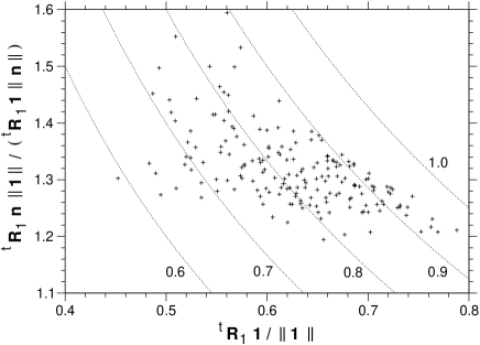
Figure 1: The ratio of ${}^{t}{\bf R}_{1}{\bf n}/\parallel{\bf n}\parallel$ to ${}^{t}{\bf R}_{1}{\bf 1}/\parallel{\bf 1}\parallel$ is shown for each of 182 proteins, which are representatives of single domain proteins from each family of classes 1 – 4 in the SCOP version 1.69. ${\bf R}_{1}$ and ${\bf n}$ are the principal eigenvector and contact number vector of the native $C$ matrix, respectively. The dotted lines indicate the iso-value lines for ${}^{t}{\bf R}_{1}{\bf n}/\parallel{\bf n}\parallel$, whose values are shown in the figure.

Eq. (24) indicates that the eigenvalues of the $C$ matrix are proportional to the square root of the second moment of contact numbers. The proportional coefficient for the principal eigenvalue of the $C$ matrix — that is, ${}^{t}{\bf R}_{1}{\bf n}\parallel{\bf 1}\parallel/(^{t}{\bf R}_{1}{\bf 1}\parallel{\bf n}\parallel)$ — is plotted for each protein in Fig. 1. The dotted lines are iso-cosine lines for the angle between the principal eigenvector of the $C$ matrix and contact number vector, whose values are written in the figure. The ratios are scattered between 1.2 and 1.6, although the value of the ratio depends on the value of the abscissa, ${}^{t}{\bf R}_{1}{\bf 1}/\parallel{\bf 1}\parallel$. The cosine of the angle is upper bounded by the value of 1, and therefore the value of the ratio of the cosines becomes correlated with the value of the denominator of the ratio — i.e., ${}^{t}{\bf R}_{1}{\bf 1}/\parallel{\bf 1}\parallel$. The important fact is that the ratio takes values larger than 1, making the principal eigenvalue larger. Here, it should be noted that the lower bound of the conformational energy linearly depends on the principal eigenvalue of the $C$ matrix; see Eq. (17). Thus, the larger the principal eigenvalue is, the lower the conformational energy becomes. In practice, this condition seems to yield a high correlation between the principal eigenvector and the contact number vector; most of the values of the ${}^{t}{\bf R}_{1}{\bf n}/\parallel{\bf n}\parallel$, are greater than 0.7.

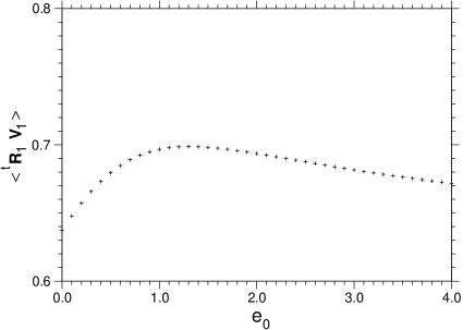
Figure 2: The mean of ${}^{t}{\bf R}_{1}{\bf V}_{1}$ over 182 proteins is plotted with plus marks against $e_{0}$. These proteins are representatives of single domain proteins from each family of classes 1 – 4 in the SCOP version 1.69. ${\bf R}_{1}$ is the principal eigenvector of the native $C$ matrix. ${\bf V}_{1}$ is the principal eigenvector for the $E$ matrix with the value of $e_{0}$ specified on the abscissa.

Now let us think about the relationship between the $C$ matrix and pairwise interactions. Pairwise interactions between residues are evaluated by using a statistical estimate MJ:03 of contact energies with a correction MJ:99 for the Bethe approximation. Figure 2 shows the average of ${}^{t}{\bf R}_{1}{\bf V}_{1}$ over all the proteins for each value of $e_{0}$. The average $\langle^{t}{\bf R}_{1}{\bf V}_{1}\rangle$ takes the maximum value $0.699$ at $e_{0}=1.3$, although its decrements according to the increase of $e_{0}$ are not large. In the following, $e_{0}=1.3$ is used to calculate the eigenvectors of the $E$ matrices.

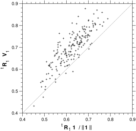
Figure 3: The value of ${}^{t}{\bf R}_{1}{\bf V}_{1}$ is plotted against ${}^{t}{\bf R}_{1}{\bf 1}/\|{\bf 1}\|$ for each of 182 proteins, which are representatives of single domain proteins from each family of classes 1 – 4 in the SCOP version 1.69. ${\bf R}_{1}$ is the principal eigenvector of the native $C$-matrix. ${\bf V}_{1}$ is the principal eigenvector for $E$-matrix with $e_{0}=1.3$. The dotted line shows the line of equal values between the ordinate and abscissa.

The value of ${}^{t}{\bf R}_{1}{\bf V}_{1}$ for each protein is plotted against the value of ${}^{t}{\bf R}_{1}{\bf 1}/\|{\bf 1}\|$ in Fig. 3. The value of ${}^{t}{\bf R}_{1}{\bf V}_{1}$ is larger for most of the proteins than that of ${}^{t}{\bf R}_{1}{\bf 1}/\|{\bf 1}\|$. If the direction of ${\bf R}_{1}$ is randomly distributed in the domain of $R_{i1}>0$, the probability that ${}^{t}{\bf R}_{1}{\bf V}_{1}$ is larger than ${}^{t}{\bf R}_{1}{\bf 1}/\|{\bf 1}\|$ must be smaller than $0.5$. Then, in such a random distribution, the probability to observe Fig. 3, in which 175 of 182 proteins fall into the region of ${}^{t}{\bf R}_{1}{\bf V}_{1}>\ ^{t}{\bf R}_{1}{\bf 1}/\|{\bf 1}\|$, must be smaller than ${}_{182}C_{175}(0.5)^{175}=\exp(-91.6)$. Also t-tests are performed for the correlation coefficients between ${\bf R}_{1}$ and ${\bf V}_{1}$ in all proteins. The geometric mean of probabilities for a significance over 182 proteins examined here is equal to $\exp(-18.4)$. Thus, it is statistically significant that the direction of the vector ${\bf R}_{1}$ is closer to ${\bf V}_{1}$ rather than ${\bf 1}$ whose elements do not depend on residues in proteins, This fact indicates that a parallel orientation between the principal eigenvectors of the $C$ and $E$ matrices is favored.

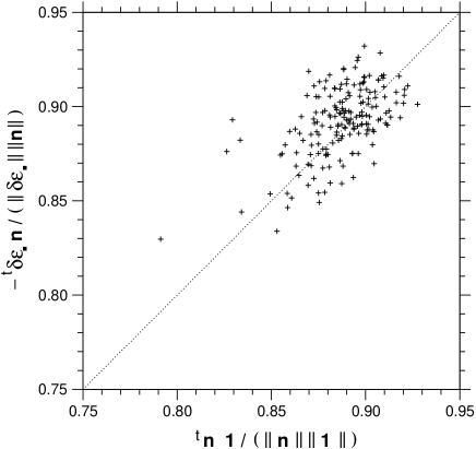
Figure 4: The value of $-^{t}\delta\vec{\mathcal{E}}_{\bullet}{\bf n}/(\parallel\delta\vec{\mathcal{E}}_{\bullet}\parallel\parallel{\bf n}\parallel)$ is plotted against ${}^{t}{\bf n}{\bf 1}/(\parallel{\bf n}\parallel\parallel{\bf 1}\parallel)$ for each of 182 proteins, which are representatives of single domain proteins from each family of classes 1 – 4 in the SCOP version 1.69. $e_{0}=1.3$ is used for the $E$-matrix. The dotted line shows the line of equal values between the ordinate and abscissa.

Eq. (28) indicates that the mean contact energy vector $\delta\vec{\mathcal{E}}_{\bullet}(\equiv^{t}(\ldots,\frac{1}{N}\sum_{k}\delta\mathcal{E}_{ik}(S),\ldots))$ being antiparallel to the contact number vector is favorable to decrease the conformational energy. Figure 4 does not show a strong but statistically significant tendency that the value of $-^{t}\delta\vec{\mathcal{E}}_{\bullet}{\bf n}/(\parallel\vec{\mathcal{E}}_{\bullet}\parallel\parallel{\bf n}\parallel)$ tends to be larger than ${}^{t}{\bf n}{\bf 1}/(\parallel{\bf n}\parallel\parallel{\bf 1}\parallel)$; in t-tests for correlation coefficients between $\delta\vec{\mathcal{E}}_{\bullet}$ and ${\bf n}$, the geometric mean of probabilities for a significance over 182 proteins is equal to $\exp(-27.9)$. If the $E$ matrix can be approximated by the principal eigenvector term, this fact indicates that the contact number vector tends to be parallel to the principal eigenvector of the $E$ matrix. Actually this is the case for the present estimate of the contact energies; the figure of ${}^{t}{\bf V}_{1}{\bf n}/\parallel{\bf n}\parallel$ versus ${}^{t}{\bf n}{\bf 1}/(\parallel{\bf n}\parallel\parallel{\bf 1}\parallel)$ is not shown. In t-tests for correlation coefficients between ${\bf V}_{1}$ and ${\bf n}$, the geometric mean of probabilities for a significance is equal to $\exp(-28.8)$.

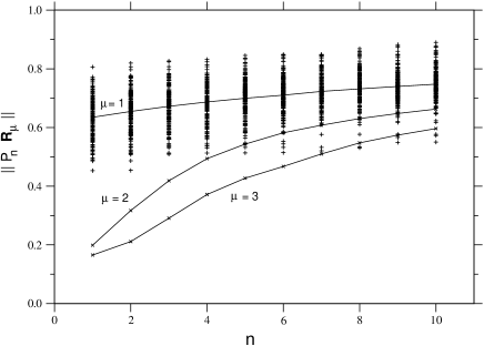
Figure 5: The norms of the $C$ matrix eigenvectors, ${\bf R}_{\mu}$, projected on the subspace consisting of the $n$ lowest-frequency normal modes of a Kirchihoff matrix corresponding to the $C$-matrix, are plotted against $n$; the primary eigenspace, indicated by $n=1$, of the Kirchihoff matrix is the one consisting of all eigenvalues equal to zero. $P_{n}$ means a projection operator on the $n$ lowest-frequency normal modes of the Kirchhoff matrix. Plus marks indicate the norm of the principal eigenvector of the $C$-matrix of each of 182 proteins projected on each subspace consisting of the $n$ lowest-frequency normal modes indicated on the abscissa. The solid curves with cross marks indicate those norms averaged over all the proteins; their curves from the left to the right show those values for the first, the second, and the third principal eigenvectors of the $C$ matrix, respectively.

Here, we have shown that the principal eigenvector among other eigenvectors of the $C$ matrix seems to be a main contributor to minimize the conformation energy. It is important to take notice that the principal eigenvector of the $C$ matrix corresponds to the lower-frequency normal modes of protein motion. Let us think about a Kirchhoff matrix that is defined as

$$K_{ij} \equiv n_{i}\delta_{ij}-\Delta_{ij}{,}$$ (44)

where $\delta_{ij}$ is a Kronecker’s delta. The eigenvalue of the Kirchhoff matrix is equal to the square of normal mode angular frequency in a system in which $i$th and $j$th units are connected to each other by a spring with a spring constant equal to $\Delta_{ij}$. If the contact number $n_{i}$ is equal to a constant $n_{c}$ irrespective of unit $i$, then the eigenvalue of the Kirchhoff matrix is equal to $n_{c}-\lambda_{\mu}$. In other words, in this case the principal eigenvector of the $C$ matrix corresponding to the largest eigenvalue is equal to the eigenvector of the Kirchhoff matrix corresponding to the smallest eigenvalue — that is, the lowest-frequency normal mode corresponding to a motion that leads to a large conformational change T:96 . In actual proteins, the contact number $n_{i}$ depends on the unit $i$, and then the correspondence between the eigenvectors of the $C$ matrix and the Kirchhoff matrix would become vague, but it will be expected that the principal eigenvector of the $C$ matrix belongs to a subspace consisting of lower-frequency normal modes.

In Fig. 5, plus marks indicate the norm of the principal eigenvector of the $C$ matrix of each of 182 proteins projected on each subspace consisting of the $n$ lowest-frequency normal modes indicated on the abscissa. In most of the proteins, the principal eigenvector of the $C$ matrix corresponds to the lower-frequency normal modes of the Kirchhoff matrix. The solid curves with cross marks indicate those norms averaged over all proteins; their curves from the left to the right show those values for the first, second, and third principal eigenvectors of the $C$ matrix, respectively. The solid curve for the principal eigenvector shows that about 70% of the principal eigen vector of the $C$ matrix can be explained by only ten lowest-frequency normal modes. Thus, the principal eigenvector of the $C$ matrix is not only an important contributor to minimize conformation energy, but also corresponds to the lower-frequency normal modes of protein motion.

V Discussion

The lower bounds of the total contact energy lead to a relationship between $E$ and $C$ matrices such that the contact potential looks like a Go-like potential. Such a relationship may be realized only for ideal proteins, but in real proteins, atom- and residue-connectivities and steric hindrance not included in the contact energy can significantly reduce conformational space; the number of possible $C$-matrices is of the order of $2^{N(N-1)/2}$ but the conformational entropy of self-avoiding chains is proportional to at most $N$, where $N$ is the chain length. As a result, Eq. (18) is expected to be approximately satisfied only for some singular spaces, probably for singular values taking relatively large values, but at least for the principal singular space. It was confirmed in the representative proteins that the inner products of the principal eigenvectors of $E$ and $C$ matrices are significantly biased toward the value 1 at a certain value of the threshold energy $\varepsilon_{0}$ for contacts, where their average over all proteins has a maximum; see Fig. 3. Parallel relationships were also indicated and confirmed between the principal eigenvector ${\bf R}_{1}$ and the contact number vector ${\bf n}$ of the $C$ matrix and between the mean contact energy vector $\delta\vec{\mathcal{E}}_{\bullet}$ and the contact number vector ${\bf n}$; see Figures 1 and 4. In these analyses, a statistical potential was used to evaluate the contact energies between residues, and the coarse grain of the evaluations limits the present analysis to a relationship between the principal eigenvectors of the $E$ and $C$ matrices, and also can make the relationship between these matrices vague. However, the results clarify the significance of the principal eigenvectors of the $E$ and $C$ matrices and contact number vector in protein structures. Here, it may be worthy of note that the principal eigenvector of the $C$ matrix corresponds to the lower-frequency normal modes of protein structures.

The condition for the lowest bound of energy, Eq. (10), indicates that $\varepsilon_{0}$ in real proteins corresponds to a threshold of contact energy for a unit pair to tend to be in contact in the native structures. In principle, such a threshold for contact energy depends on the size of the protein and protein architecture; it should be noted that many types of interactions in real proteins are missed in representing interactions by contact potentials. The estimate of $e_{0}$ shown in Fig. 2 is an estimate only for the present specific type of a contact potential. The important things are that the total contact energy is bounded by Eq. (8) with a constant term, and that spectral relationships of Eqs. (18) and 21 between $E$ and $C$ matrices are expected for the conformations of the lower bounds if the $E$ matrix is decomposed with a constant term as shown in Eq. (13).

Besides that, the spectral representation of $C$ and $E$ matrices reveals that pairwise residue-residue interactions, which depends only on the types of interacting amino acids but not on other residues in a protein, are insufficient and other interactions including residue connectivities and steric hindrance are needed to make native structures unique lowest-energy conformations.

References

- (1)
- (2) A. R. Kinjo and S. Miyazawa, Chem. Phys. Lett. 451, 132 (2008).
- (3) N. Go, Annu. Rev. Biophys. Bioeng. 12, 183 (1983).
- (4) A. G. Murzin, S. E. Brenner, T. Hubbard and C. Chothia, J. Mol. Biol. 247, 536 (1995).
- (5) S. Miyazawa and R. L. Jernigan, Proteins 34, 49 (1999).
- (6) S. Miyazawa and R. L. Jernigan, Proteins 50, 35 (2003).
- (7) A. Kabakçioǧlu, I. Kanter, M. Vendruscolo and E. Domany, Phys. Rev. E 65, 041904 (2002).
- (8) M. Porto, U. Bastolla, H. E. Roman and M. Vendruscolo, Phys. Rev. Lett. 92, 218101 (2004).
- (9) A. R. Kinjo and K. Nishikawa, Bioinformatics 21, 2167 (2005).
- (10) A. Vullo, I. Walsh and G. Pollastri, BMC Bioinformatics 7, 180-1 (2006).
- (11) K. Nishikawa and T. Ooi, J. Peptide Protein Res. 16, 19 (1980).
- (12) K. Nishikawa and T. Ooi, J. Biochem. 100, 1043 (1986).
- (13) A. R. Kinjo, K. Horimoto and K. Nishikawa, Proteins 58, 158 (2005).
- (14) H. Cao, Y. Ihm, C. Z. Wang, J. R. Morris, M. Su, D. Dobbs and K. M. Ho, Polymer 45, 687 (2004).
- (15) H. Cao, C. Z. Wang, D. Dobbs, Y. Ihm and K. M. Ho, Phys. Rev. E 74, 031921 (2006).
- (16) U. Bastolla, M. Porto, H. E. Roman and M. Vendruscolo, Proteins 58, 22 (2005).
- (17) F. Seno, M. Vendruscolo, A. Maritan and J. R. Banavar, Phys. Rev. Lett. 77, 1901 (1996).
- (18) J. M. Deutsch and T. Kurosky, Phys. Rev. Lett. 76, 323 (1996).
- (19) M. Morrissey and E. I. Shakhnovich, Folding & Design 1, 391 (1996).
- (20) S. Miyazawa and R. L. Jernigan, Proteins 36, 357 (1999).
- (21) L. Mirny, V. Abkevich and E. I. Shakhnovich, Folding & Design 1, 103 (1996).
- (22) R. A. Horn and C. R. Johnson, Matrix analysis (Cambridge: Cambridge University Press, 1985).
- (23) S. Miyazawa and R. L. Jernigan, J. Chem. Phys. 122, 024901-1 (2005).
- (24) P. J. Munson and R. K. Singh, Protein Sci. 6, 1467 (1997).
- (25) G. Chikenji, Y. Fujitsuka and S. Takada, Proc. Natl. Acad. Sci. USA 103, 3141 (2006).
- (26) P. J. Fleming, H. Gong and G. D. Rose, Protein Sci. 15, 1829 (2006).
- (27) L. A. Mirny and E. I. Shakhnovich, J. Mol. Biol. 264, 1164 (1996).
- (28) D. Toby and R. Elber, Proteins 41, 40 (2000).
- (29) D. Toby, G. Shafran, N. Linial and R. Elber, Proteins 40, 71 (2000).
- (30) B. Bollobás, Modern graph theory (Berlin: Springer Verlag, 1998).
- (31) S. Miyazawa and R. L. Jernigan, Macromolecules 18, 534 (1985).
- (32) S. Miyazawa and R. L. Jernigan, J. Mol. Biol. 256, 623 (1996).
- (33) H. Li, C. Tang and N. Wingreen, Phys. Rev. Lett. 79, 765 (1997).
- (34) L. Holm and C. Sander, Proteins 19, 256 (1994).
- (35) N. Kannan and S. Vishveshwarar, J. Mol. Biol. 292, 441 (1999).
- (36) N. Kannan and S. Vishveshwarar, Protein Eng. 13, 753 (2000).
- (37) H. M. Berman, J. Westbrook, Z. Feng, G. Gilliland, T. N. Bhat, H. Weissig, I. N. Shindyalov and P. E. Bourne, Nucl. Acid Res. 28, 235 (2000).
- (38) M. M. Tirion, Phys. Rev. Lett. 77, 1905 (1996).