Exactness of Belief Propagation
for Some Graphical Models with Loops

Abstract

It is well known that an arbitrary graphical model of statistical inference defined on a tree, i.e. on a graph without loops, is solved exactly and efficiently by an iterative Belief Propagation (BP) algorithm convergent to unique minimum of the so-called Bethe free energy functional. For a general graphical model on a loopy graph the functional may show multiple minima, the iterative BP algorithm may converge to one of the minima or may not converge at all, and the global minimum of the Bethe free energy functional is not guaranteed to correspond to the optimal Maximum-Likelihood (ML) solution in the zero-temperature limit. However, there are exceptions to this general rule, discussed in [12] and [2] in two different contexts, where zero-temperature version of the BP algorithm finds ML solution for special models on graphs with loops. These two models share a key feature: their ML solutions can be found by an efficient Linear Programming (LP) algorithm with a Totally-Uni-Modular (TUM) matrix of constraints. Generalizing the two models we consider a class of graphical models reducible in the zero temperature limit to LP with TUM constraints. Assuming that a gedanken algorithm, g-BP, finding the global minimum of the Bethe free energy is available we show that in the limit of zero temperature g-BP outputs the ML solution. Our consideration is based on equivalence established between gapless Linear Programming (LP) relaxation of the graphical model in the $T\to 0$ limit and respective LP version of the Bethe-Free energy minimization.

1 Introduction

Belief Propagation (BP) is an algorithm finding ML solution or marginal probabilities on a graph without loops, a tree. The algorithm was introduced in [8] as an efficient heuristic for decoding of sparse (so called graphical) codes and it was independently considered in the context of graphical models of artificial intelligence [16]. Originally the algorithm was primarily thought of as an iterative procedure. [24, 23], inspired by earlier works of [3] and [17] in statistical physics, suggested to use a more fundamental notion of the Bethe free energy. Extrema of the Bethe free energy represent fixed points of the iterative BP algorithm on graphs with cycles. Equations describing the stationary points of the Bethe free energy and the fixed points of the iterative BP are called Belief Propagation, or Bethe-Peierls, BP equations.

The significance of BP, understood as an algorithm looking for a minimum of the Bethe free energy, was further elucidated within the framework coined loop calculus [5, 6]. It was shown that algorithm finding an extremum of the Bethe Free Energy is not just an approximation/heursistics in the loopy case, but it allows explicit reconstruction of the exact inference in terms of a series, where each term corresponds to a loop on the graph.

If the graphical model is dense there are many loops, and thus many contributions to the loop series. However, not all loops are equal. Thus, considering models characterized by the same graph but different factor functions or local weights (exact definitions will follow) one expects strong sensitivity of an individual loop contribution (and its significance within the loop series) on the factor functions. In this context it is of interest to study the following question: are there graphical models, defined on an arbitrary graph but with specially tuned factor functions, such that BP provides exact inference?

Positive answer to this question was given, independently and for two different models, by [12] and [2]. It was shown in [12] that for a graphical model defined on an arbitrary graph in terms of binary variables with pairwise sub-modular interaction a properly defined version of BP (linear programming relaxation underlying the tree-reweighted method of [20]) yields a globally optimal Maximum Likelihood solution. This model is equivalent to the Ferromagnetic Random Field Ising (FRFI) model popular in statistical physics of disordered systems, see e.g. [10]. Maximum weight matching problem on a bipartite graph was analyzed in [2] and later in [18], where it was shown that, in spite of the fact that the underlying graph has many short cycles, an algorithm of BP type does converge to correct ML assignment. This consideration was also extended to the problem of weighted b-matchings on an arbitrary graph (which is yet another problem solvable exactly by BP) in [1, 11]. Closely related general results, discussing convexified version of Bethe Free energy and an iterative convex-BP scheme converging to respective LP, were reported in [22, 9].

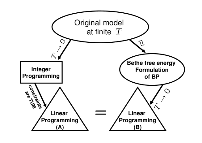
Figure 1: Scheme illustrating the sequence of transformations and relations discussed in the paper.

In this paper we use the Bethe free energy approach of [23] to suggest a complementary and unifying explanation to these remarkable, and somehow surprising, results of [12, 2]. In two subsequent Sections we consider two models, FRFI discussed in [12] and a binary model with Totally Uni-Modular (TUM) constraints generalizing the weight matching problem considered in [2]. Statistical weights are defined for both models in terms of a characteristic temperature, $T$. Our strategy in dealing with both models is illustrated in Fig. 1. It consists of the following three steps.

• Starting from the original setting we first go anti-clockwise, getting an Integer Programming (IP) formulation for the ML, $T\to 0$, version of the problem. The most important feature of the two models is that the LP relaxation of the respective IP, shown as LP-A in the Figure, is tight/exact. In both cases this reduction from IP to LP is exact due to the Total-Uni-Modularity (TUM) feature of the underlying matrix of constraints.

• Then we return to the original setting and start moving clockwise (see the Figure), first to the Bethe free energy formulation of the problem. We call the gedanken algorithm, finding global minima of the Bethe free energy, g-BP In the $T\to 0$ limit the Bethe free energy turns to respective self-energy (the entropy term multiplied by temperature is irrelevant) which is a linear functional of beliefs. Thus one gets to an LP problem here as well, the one shown as LP-B in the Figure. This transformation from g-BP to LP-B is analogous to similar relation between g-BP and LP-decoding introduced in the coding theory in [7, 19].

• Finally, we show that LP-A and LP-B are identical, thus demonstrating that g-BP in the $T\to 0$ limit outputs the ML solution.

Note, that convexity of the Bethe free energy at finite temperature, playing the key role in analysis of [12, 22, 9], is not a required part our consideration. Moreover, the Bethe free energy of the binary model with TUM constraints is generally not convex.

2 Ferromagnetic Random Field Ising model

Consider an undirected graph ${\cal G}$, consisting of $n$ vertexes, ${\cal V}=\{1,\cdots,n\}$ and weighted edges, ${\cal E}$, with the weight matrix $(J_{ij}|i,j=1,\cdots,n)$ such that whenever the two vertexes are connected by an edge, i.e. $i\in j$ or $j\in i$, $J_{ij}>0$, and $J_{ij}=0$, otherwise. It is also useful to introduce the directed version of the graph, ${\cal G}_{d}$, where any undirected edge of ${\cal G}$ is replaced by two directed edges of ${\cal G}_{d}$, with the weights $J_{i\to j}=J_{j\to i}=J_{ij}/2$ respectively. The Ferromagnetic Random Field Ising (FRFI) model is defined by the following statistical weight associated with any configuration of ${\bm{\sigma}}=(\sigma_{i}=\pm 1|i=1,\cdots,n)$ on ${\cal V}$:

$$p({\bm{\sigma}})=Z^{-1}\exp\left(\frac{1}{2T}\sum_{(i,j)\in{\cal G}}J_{ij}\sigma_{i}\sigma_{j}+\frac{1}{T}\sum_{i}h_{i}\sigma_{i}\right)$$

$$=Z^{-1}\exp\left(\frac{1}{2T}\sum_{(i\to j)\in{\cal G}_{d}}J_{i\to j}\sigma_{i}\sigma_{j}+\frac{1}{T}\sum_{i}h_{i}\sigma_{i}\right),$$ (1)

where $h_{i}$ can be positive or negative; $T$ is the temperature; $Z$ is the partition function, enforcing the probability normalization condition, $\sum_{\bm{\sigma}}p({\bm{\sigma}})=1$; and $(i,j)$/$(i\to j)$ marks an undirected/directed edge of ${\cal G}$/${\cal G}_{d}$ connecting the two neighbors $i$ and $j$.

2.1 From FRFI to the Min-Cut Problem

Maximum Likelihood (ground state) solution of Eq. (1) turns into the problem of quadratic integer programming

$$\left.\min_{\bm{\sigma}}\left(-\frac{1}{2}\sum_{(i\to j)\in{\cal G}_{d}}J_{i\to j}\sigma_{i}\sigma_{j}-\sum_{i\in{\cal G}_{d}}h_{i}\sigma_{i}\right)\right|_{\forall\ i\in{\cal G}_{d}:\ \ \sigma_{i}=\pm 1}.$$ (2)

It is well known that any sub-modular energy function (and the quadratic function in Eq. (2) is of this type) can be minimized in polynomial time by reducing the task to the maximum flow/min-cut problem [4, 10]. In this Subsection we will reproduce these known results.

To unify linear and quadratic terms in Eq. (2), one constructs a new graph, ${\cal G}^{\prime}_{d}$, adding two new nodes to ${\cal G}_{d}$: source (s) and destination (d), with $\sigma_{s}=+1$ and $\sigma_{d}=-1$ respectively. The (s)-node is linked to all the nodes of ${\cal G}_{d}$ with $h_{i}>0$, while any node of ${\cal G}_{d}$ with $h_{i}<0$ is linked to (d). Weights of the newly introduced directed edges of ${\cal G}^{\prime}_{d}$ are

$$J_{s\to i}=2h_{i},\mbox{ if }h_{i}>0;\quad J_{i\to d}=2|h_{i}|,\mbox{ if }h_{i}<0.$$ (3)

This results in the following version of Eq. (2)

$$\left.\min_{\bm{\sigma}}\left(-\frac{1}{2}\sum_{(i\to j)\in{\cal G}^{\prime}_{d}}J_{i\to j}\sigma_{i}\sigma_{j}\right)\right|_{\forall\ i\in{\cal G}_{d}:\ \ \sigma_{i}=\pm 1;\sigma_{s}=+1;\sigma_{d}=-1}.$$ (4)

Reduction from quadratic integer programming (4) to an integer linear programming is the next step. This is achieved via transformation to the edge variables,

$$\forall(i\to j)\in{\cal G}_{d}:\quad\eta_{i\to j}=\left\{\begin{array}[]{cc}1,&\sigma_{i}=1,\sigma_{j}=-1\\ 0,&\mbox{otherwise}.\end{array}\right.$$ (7)

The relations can also be restated

$$\forall(i\to j),(j\to i)\in{\cal G}_{d}:\quad\sigma_{i}\sigma_{j}+\sigma_{j}\sigma_{i}=2-4(\eta_{i\to j}+\eta_{j\to i})$$ (8)

$$\forall(d\to i),(j\to t):\quad\sigma_{i}\sigma_{d}=1-2\eta_{d\to i},\quad\sigma_{s}\sigma_{j}=1-2\eta_{j\to s},$$ (9)

Therefore, taking into account that , $J_{i\to j}=J_{j\to i}$ for any $(i\to j),(j\to i)\in{\cal G}_{d}$, substituting Eqs. (7,8,9) into Eq. (4) and changing variables from $\sigma_{i}=\pm 1$ to $p_{i}=(1-\sigma_{i})/2=0,1$ one arrives at

$$-\frac{1}{2}\sum\limits_{(i\to j)\in{\cal G}^{\prime}_{d}}J_{i\to j}+\left.\min\limits_{\{\eta,p\}}\sum_{(i\to j)\in{\cal G}^{\prime}_{d}}J_{i\to j}\eta_{i\to j}\right|_{\begin{array}[]{c}\forall i\in{\cal G}^{\prime}_{d},p_{i}=0,1;\\ \forall(i\to j)\in{\cal G}^{\prime}_{d}:\ \ p_{i}-p_{j}+\eta_{i\to j}=0,1;\\ p_{s}=0,\quad p_{d}=1\end{array}}.$$ (10)

This expression is nothing but the integer programming formulation of the famous min-cut problem, calculating the minimum weight cut splitting all the nodes of the directed graph into two parts such that the group including the source node has all variables in the $0$ state while the other group, including the destination node, has all variables in the $1$ state.

Any $\{\eta,p\}$ configuration which satisfies conditions in Eq. (10) requires that either $\eta_{i\to j}=0$ and $\eta_{j\to i}=1$ or $\eta_{i\to j}=1$ and $\eta_{j\to i}=0$ for any pair of directed edges $(i\to j),(j\to i)\in{\cal G}_{d}$. This suggests that Eq. (10) can be restated in terms of the undirected graph $G^{\prime}$, equivalent to the original ${\cal G}$ supplemented by the source and destination vertexes and edges with the following positive weights

$$J_{si}=2h_{i},\mbox{ if }h_{i}>0;\quad J_{id}=2|h_{i}|,\mbox{ if }h_{i}<0.$$ (11)

One derives the following undirected version of Eq. (10)

$$-\frac{1}{2}\sum\limits_{(i,j)\in{\cal G}^{\prime}}J_{ij}+\left.\min\limits_{\{\eta,p\}}\sum_{(i,j)\in{\cal G}^{\prime}}J_{ij}\eta_{i\to j}\right|_{\begin{array}[]{c}\forall i\in{\cal G}^{\prime},p_{i}=0,1;\\ \forall(i,j)\in{\cal G}^{\prime}:\ \ p_{i}-p_{j}+\eta_{ij}=0,1;\\ p_{s}=0,\quad p_{d}=1\end{array}}.$$ (12)

The min-cut problem (12) is solvable in polynomial time. This means, in particular, that solution of the Integer Programming Eq. (12) and solution of the respective relaxed LP-A,

$$-\frac{1}{2}\sum\limits_{(i,j)\in{\cal G}^{\prime}}J_{ij}+\left.\min\limits_{\{\eta,p\}}\sum_{(i,j)\in{\cal G}^{\prime}}J_{ij}\eta_{ij}\right|_{\left\{\begin{array}[]{c}\forall i\in{\cal G}^{\prime},1\geq p_{i}\geq 0;\\ \forall(i,j)\in{\cal G}^{\prime}:\ p_{i}-p_{j}+\eta_{ij}\geq 0;\\ p_{s}=0,\quad p_{d}=1\end{array}\right.},$$ (16)

are identical. The tightness of the relaxation is, e.g., discussed in [15]. (See Ch. 6.1 and specifically Theorems 6.1,6.2 in [15].) Also, this observation is closely related to the fact that the matrix of constraints in the max-flow problem, which is dual to Eq. (12), is Totally Uni-Modular (TUM), i.e. such that any square minor of the matrix has determinant which is $0,+1$ or $-1$. (See e.g. Ch. 13.2 of [15] for discussion of the TUM IP/LP problems.)

2.2 Bethe Free Energy and Belief Propagation for FRFI

Discussing the FRFI model defined in Eq. (1) and following the general heuristic approach to the graphical models, suggested in [23], one introduces beliefs, i.e. estimated probabilities, for vertexes and edges, $b_{i}(\sigma_{i})$, $b_{ij}(\sigma_{i},\sigma_{j})$, related to each other according to

$$\forall i\ \ \&\ \ \forall j\in i:\quad b_{i}(\sigma_{i})=\sum_{\sigma_{j}}b_{ij}(\sigma_{i},\sigma_{j}),$$ (17)

and also satisfying the obvious normalization condition

$$\forall i:\quad\sum_{\sigma_{i}}b_{i}(\sigma_{i})=1.$$ (18)

Then the Bethe free energy functional of the beliefs is defined as

$${\cal F}=E-TS,\quad E=-\frac{1}{2}\sum_{(i,j)}\sum_{\sigma_{i},\sigma_{j}}b_{ij}(\sigma_{i},\sigma_{j})J_{ij}\sigma_{i}\sigma_{j}-\sum_{i}\sum_{\sigma_{i}}b_{i}(\sigma_{i})h_{i}\sigma_{i},$$ (19)

$$S=\sum_{(i,j)}\sum_{\sigma_{i},\sigma_{j}}b_{ij}(\sigma_{i},\sigma_{j})\ln b_{ij}(\sigma_{i},\sigma_{j})-\sum_{i}\sum_{\sigma_{i}}b_{i}(\sigma_{i})\ln b_{i}(\sigma_{i}).$$ (20)

Introducing Lagrangian multipliers associated with the constraints (17,18), one defines the Lagrangian functional

$${\cal L}={\cal F}+\sum_{i}\sum_{j\in i}\sum_{\sigma_{i}}\eta_{ij}(\sigma_{i})\left(b_{i}(\sigma_{i})-\sum_{\sigma_{j}}b_{ij}(\sigma_{i},\sigma_{j})\right)+\sum_{i}\lambda_{i}\left(\sum_{\sigma_{i}}b_{i}(\sigma_{i})-1\right).$$ (21)

Looking for the stationary point of the Lagrangian over all the parameters (the beliefs and the Lagrangian multipliers) will define the Belief Propagation (BP) equations. Iterative solution of the BP equations constitutes the celebrated BP algorithm, which is often used as an efficient heuristic for estimating marginal probabilities in sparse graphical models.

2.2.1 Ground State

In the $T\to 0$ limit the entropy terms in the expression for the Bethe free energy in Eqs. (19) can be neglected and the task of finding the absolute minimum of the Bethe free energy functional turns into minimization of the self-energy, $E$ from Eq. (19), under the set of constraints (17,18). Both the optimization functional and the constraints are linear in the beliefs, therefore one gets here the following Linear Programming optimization:

$$\left.\min\limits_{\{b_{i};b_{ij}\}}\left(-\!\!\!\!\sum_{(i,j)\in{\cal G}}\sum_{\sigma_{i},\sigma_{j}}b_{ij}(\sigma_{i},\sigma_{j})\frac{J_{ij}}{2}\sigma_{i}\sigma_{j}\!-\!\sum_{i\in{\cal G}}\sum_{\sigma_{i}}b_{i}(\sigma_{i})h_{i}\sigma_{i}\right)\right|_{\begin{array}[]{c}\forall i,(i,j)\in{\cal G}:\\ b_{i}(\sigma_{i})=\sum_{\sigma_{j}}b_{ij}(\sigma_{i},\sigma_{j})\\ \sum_{\sigma_{i}}b_{i}(\sigma_{i})=1\end{array}},$$ (22)

where it is also assumed that all the beliefs are positive and smaller than or equal to unity (as we are looking only for physically sensible solutions of the optimization problem).

Making the transformation from the original graph ${\cal G}$ to its extended version, ${\cal G}^{\prime}$, i.e. introducing new edges with weights defined in Eqs. (11), and requiring that the spin values of the source/destination are fixed to $\pm 1$ respectively, i.e. $b_{s}(+)=b_{d}(-)=1$ and $b_{s}(-)=b_{d}(+)=0$, one rewrites Eq. (22) as

$$\left.\min\limits_{\{b_{i};b_{ij}\}}\left(-\sum_{(i,j)\in{\cal G}^{\prime}}\sum_{\sigma_{i},\sigma_{j}}b_{ij}(\sigma_{i},\sigma_{j})\frac{J_{ij}}{2}\sigma_{i}\sigma_{j}\right)\right|_{\begin{array}[]{c}\forall i,(i,j)\in{\cal G}^{\prime}:\quad b_{i}(\sigma_{i})=\sum_{\sigma_{j}}b_{ij}(\sigma_{i},\sigma_{j})\\ \forall i\in{\cal G}^{\prime}:\quad\sum_{\sigma_{i}}b_{i}(\sigma_{i})=1\\ b_{s}(+)=1\ \ \&\ \ b_{d}(-)=1\end{array}}.$$ (23)

The structure of the optimization functional in Eq. (23) suggests to reduce the number of variables (beliefs), thus keeping only the edge variables

$$\mu_{ij}\equiv b_{ij}(+,-)+b_{ij}(-,+)=1-b_{ij}(+,+)-b_{ij}(-,-),$$ (24)

defined as the probabilities to observe the edge $(i,j)$ either in the state $(+,-)$ or in the state $(-,+)$. Thus, by construction, $1\geq\mu_{ij}\geq 0$. The $\mu_{ij}$ variables defined at different edges are related to each other through local beliefs, $\pi_{i}=b_{i}(-)=1-b_{i}(+)$, which all satisfy, $0\leq\pi_{i}\leq 1$. Taking all these observations into account one rewrites Eq. (23) as

$$-\frac{1}{2}\sum\limits_{(i,j)\in{\cal G}^{\prime}}\!\!J_{ij}+\left.\min\limits_{\{\mu,\pi\}}\sum_{(i,j)\in{\cal G}^{\prime}}J_{ij}\mu_{ij}\right|_{\begin{array}[]{c}\forall i\in{\cal G}^{\prime},\ \ \forall j\in i:\ \pi_{i}-\pi_{j}+\mu_{ij}\geq 0;\ \ \ 1\geq\mu_{ij}\geq 0\\ \forall i\in{\cal G}^{\prime}:\quad 1\geq\pi_{i}\geq 0\\ \pi_{s}=0,\quad\pi_{d}=1\end{array}}.$$ (25)

One finds that, up to an obvious change of variables from $\mu$ to $\eta$ and from $\pi$ to $p$, the LP-B of Eq. (25) is identical to the LP-A (16). According to the Theorem 6.1 of [15], solutions of Eq. (25), or Eq. (16), are integers, $\forall(i,j)\in\Gamma^{\prime}$ $\mu_{ij},\eta_{ij}=0,1$ and $\forall i\in G^{\prime}$ $p_{i},\pi_{i}=0,1$.

Summarizing, it was just shown that as $T\to 0$ the BP solution of the FRFI model, understood as the global minimum of the Bethe Free energy, is also the ML solution of the model.

3 Binary model with Totally Uni-Modular Constraints

Consider $N$ binary variables combined in the vector ${\bm{\sigma}}=(\sigma_{i}=0,1|i=1,\cdots,N)$, and associate the following normalized probability to any possible value of the vector

$$p({\bm{\sigma}})=Z^{-1}\exp\left(-T^{-1}\sum_{i}h_{i}\sigma_{i}\right)\prod\limits_{\alpha}\delta\left(\sum_{i}J_{\alpha i}\sigma_{i},m_{\alpha}\right),$$ (26)

where $\delta(x,y)$ is one if $x=y$ and it is zero otherwise; $\alpha=1,\cdots,M$ ; matrix $\hat{J}\equiv\left(J_{\alpha i}=0,1|i=1,\cdots,N;\alpha=1,\cdots,M\right)$ is Totally Uni-Modular (TUM), i.e. determinant of any square minor of the matrix is $0,1$ or $-1$; the vector ${\bm{m}}=(m_{\alpha}|\alpha=1,\cdots,M)$ is constructed from positive integers, so that $\forall\alpha$: $m_{\alpha}\leq q_{\alpha}\equiv\sum_{i}J_{\alpha i}$. The partition function $Z$ is introduced in Eq. (26) to guarantee normalization, $\sum_{\bm{\sigma}}p({\bm{\sigma}})=1$.

The model Eq. (26) can be viewed as a graphical model defined on the bipartite graph consisting of “bits”, $\{i\}$, and “checks”, $\{\alpha\}$. Also, there may be other graphical interpretations. Thus, for the weighted matching problem, e.g. studied in [2], the binary variables in the formulation of Eq. (26), are associated with edges of the complete bipartite graph. (In this case of the weighted matching, one can show that the resulting matrix of constraints is indeed TUM.)

3.1 Efficient ML solution

We, first of all, observe that the problem of finding the Maximum Likelihood of Eq. (26) is equivalent to the following Integer Programming (IP)

$$\left.\min_{\bm{\sigma}}\sum_{i}h_{i}\sigma_{i}\right|_{\left\{\begin{array}[]{c}\forall i:\ \ \sigma_{i}=0,1\\ \forall\alpha:\ \ \sum_{i}J_{\alpha i}\sigma_{i}=m_{\alpha}\end{array}\right.}.$$ (29)

Relaxing the IP to respective LP-A. with $\sigma_{i}=0,1$ changed to $s_{i}=[0;1]$,

$$\left.\min_{\bm{\sigma}}\sum_{i}h_{i}s_{i}\right|_{\left\{\begin{array}[]{c}\forall i:\ \ 0\leq s_{i}\leq 1\\ \forall\alpha:\ \ \sum_{i}J_{\alpha i}s_{i}=m_{\alpha}\end{array}\right.}.$$ (32)

one finds that the relaxation is tight. In other words, the solutions of the IP problem and the LP problem are exactly equivalent. This is due to the Theorem (see e.g. Theorem 13.1 of [15]) stating that if $\hat{J}$ is TUM and ${\bm{m}}$ is integer, then all feasible solutions of the LP problem are integer.

3.2 Bethe Free Energy & BP

Here we discuss the Bethe free energy/Belief Propagation (BP) approach to the model defined in Eq. (26). The Bethe free energy functional is

$$F=E-TS,\quad E=\sum_{i}h_{i}b_{i}(1),$$ (33)

$$S=\sum_{\alpha}\sum_{{\bm{\sigma}}_{\alpha}}b_{\alpha}({\bm{\sigma}}_{\alpha})\ln b_{\alpha}({\bm{\sigma}}_{\alpha})-\sum_{i}\left(q_{\alpha}-1\right)b_{i}(\sigma_{i})\ln b_{i}(\sigma_{i}),$$

where a vector ${\bm{\sigma}}_{\alpha}\equiv(\sigma_{i}|\forall i\mbox{ s.t. }J_{\alpha i}=1;\sum_{i}J_{\alpha i}\sigma_{i}=m_{\alpha})$ defines the set of allowed configurations of variables marked by index $i$ associated and consistent with the given constrained $\alpha$. For any given $m_{\alpha}$ the number of such allowed vectors/configurations of ${\bm{\sigma}}_{\alpha}$ is $C_{m_{\alpha}}^{q_{\alpha}}=m_{\alpha}!/((m_{\alpha}-q_{\alpha})!q_{\alpha}!)$. As usual, $b_{\alpha}({\bm{\sigma}}_{\alpha})$ and $b_{i}(\sigma_{i})$ are beliefs (estimations for the respective probabilities) associated with the variables and the constraints. The two types of beliefs are related to each other via the following compatibility constraints:

$$\forall i\ \ \&\ \ \forall\alpha\mbox{ s.t. }J_{\alpha i}=1:\ \ b_{i}(\sigma_{i})=\sum_{{\bm{\sigma}}_{\alpha}\setminus\sigma_{i}}b_{\alpha}({\bm{\sigma}}_{\alpha}),$$ (34)

and one should also impose the normalization constraint

$$\forall\ \ i:\ \ \sum_{\sigma_{i}}b_{i}(\sigma_{i})=1.$$ (35)

Incorporating the compatibility and normalization constraints in the form of Lagrangian multipliers into the variational functional one derives the Lagrangian

$${\cal L}=F+\sum_{i}\sum_{\alpha\ni i}\mu_{\alpha i}(\sigma_{i})\left(b_{i}(\sigma_{i})-\sum_{{\bm{\sigma}}_{\alpha}\setminus\sigma_{i}}b_{\alpha}({\bm{\sigma}}_{\alpha})\right)+\sum_{i}\lambda_{i}(\sigma_{i})\left(\sum_{\sigma_{i}}b_{i}(\sigma_{i})-1\right).$$ (36)

Looking for the stationary points of the Lagrangian with respect to all the beliefs and the Lagrangian multipliers, $\lambda$,$\mu$, one arrives at the Belief Propagation equations for the problem.

3.3 $T\to 0$ limit of the Bethe free energy

In the $T\to 0$ limit the entropy term in Eq. (33) can be dropped and the problem turns into minimization of the LP type

$$\left.\min_{\{b_{i};b_{\alpha}\}}\sum_{i}h_{i}b_{i}(1)\right|_{\left\{\begin{array}[]{c}\forall i:\ \ 0\leq b_{i}(\sigma_{i})\leq 1\\ \forall i\ \ \&\ \ \forall\alpha\mbox{ s.t. }J_{\alpha i}=1:\ \ b_{i}(\sigma_{i})=\sum_{{\bm{\sigma}}_{\alpha}\setminus\sigma_{i}}b_{\alpha}({\bm{\sigma}}_{\alpha})\\ \forall\ \ i:\ \ \sum_{\sigma_{i}}b_{i}(\sigma_{i})=1\end{array}\right.}$$ (40)

It is straightforward to verify that the beliefs associated with $\alpha$ could be completely removed from Eq. (40), and the LP problem can be restated solely in terms of the $i$-related variables, $\beta_{i}\equiv b_{i}(1)=1-b_{i}(0)$.

Let us illustrate this point on example of a single $\alpha$ constraint with $m_{\alpha}=2$ and $q_{\alpha}=3$. Then the set of allowed $\alpha$-beliefs are

$$b_{\alpha}(1,1,0),b_{\alpha}(1,0,1),b_{\alpha}(0,1,1),$$ (41)

and the respective set of relations (34) between $\beta_{1},\beta_{2},\beta_{3}$ associated with the check $\alpha$ and the $\alpha$ beliefs are

$$\beta_{1}=b_{\alpha}(1,1,0)+b_{\alpha}(1,0,1),\ \ \beta_{2}=b_{\alpha}(1,1,0)+b_{\alpha}(0,1,1),\ \ \beta_{3}=b_{\alpha}(1,0,1)+b_{\alpha}(0,1,1).$$ (42)

On the other hand the normalization condition, restated in terms of the $\alpha$-beliefs (41), is

$$b_{\alpha}(1,1,0)+b_{\alpha}(1,0,1)+b_{\alpha}(0,1,1)=1.$$ (43)

Summing Eqs. (42) and accounting for Eq. (43), one finds

$$\beta_{1}+\beta_{2}+\beta_{3}=2.$$ (44)

In general, one finds that the relation between $\beta$ variables associated with an $\alpha$-constraint is

$$\sum_{i}J_{\alpha i}\beta_{i}=m_{\alpha}.$$ (45)

One derives that Eq. (40) reduces to a simpler LP-B problem stated solely in terms of the $\beta$ variables

$$\left.\min_{\beta_{i}}\sum_{i}h_{i}\beta_{i}\right|_{\left\{\begin{array}[]{c}\forall i:\ \ 0\leq\beta_{i}\leq 1\\ \forall\alpha:\ \ \sum_{i}J_{\alpha i}\beta_{i}=m_{\alpha}\end{array}\right.}.$$ (48)

Furthermore, one observes that, up to re-definition of $\beta_{i}$ to $s_{i}$, Eq. (48) is equivalent to Eq. (22). In other words, we just showed that the $T\to 0$ solution of the BP equations, understood as the global minimum of the Bethe free energy, is tight, i.e. it gives exactly the ML solution of the binary model (26).

As a side remark, one notes that it is suggestive to start exploration of the Bethe Free Energy at finite $T$ from the LP solution discussed above. It might be especially useful to initiate BP with the (easy to get) LP solution when the Bethe Free Energy optimization at finite $T$ is non-convex.

4 Summary and Path Forward

In this work we discussed easy problems when a zero-temperature BP scheme generates exact ML result. We argued that this special feature of BP is due to the fact that the related LP optimization is tight (i.e. the LP outputs ML solution as well). Our consideration was based on the flexibility and convenience provided by the so-called Bethe Free Energy formulation, naturally relating BP and LP. The results were illustrated on two examples, FRFI model and perfect matching model. Also, we briefly discussed a broader class of easy examples related to LP with TUM matrix of constraints.

We conclude briefly mentioning some future challenges which follow from our analysis.

• It is useful to continue further exploration of other models of statistical inference with loops allowing computationally efficient optimal solutions. Thus, it would be interesting to find examples of “easy” non-binary problems, also these which allow efficient and optimal finite temperature evaluation of marginal probabilities or partition function. In this context, one mentions exactness of BP marginals at any temperature known to hold for continuous variable Gaussian model on an arbitrary graph [21, 13] and also recently established, $T\to 0$, relation between an iterative algorithm of BP type and Quadratic optimization problem [14].

• Probably the most intriguing future challenge is to analyze problems that are not computationally easy, but still close, in some metric, to easy problems. Thus, the models discussed above, however considered at finite, not zero, temperature may not allow an explicit efficient solution. Similarly, perturbation of the FRFI model with some number of graph local frustrations (e.g. some number of randomly thrown negative $J_{ij}$ violating the TUM-feature of the model) sets another “close to easy” problem of theoretical and applied interest. As suggested in [12], BP can be utilized as an efficient heuristic in these “close to easy” cases. Note, that in this case finding minima of the Bethe Free energy may be a challenge, and the problem turns into the quest of devising an efficient algorithms for the optimization of non-convex functions [25, 26]. Here novel BP-convexifixation ideas developed in [20, 12, 22, 9] might be helpful. Notice also, that the loop calculus approach of [5, 6] is another useful tool which may come handy in perturbative and non-perturbative analysis of these “close to easy” problems.

• BP is the algorithm of choice for decoding of error-correction codes stated in terms of sparse graphs [8]. On the other hand, the above discussion suggests that for BP to decode optimally, or close to optimally, the graphical structure should not necessarily be sparse. Therefore, an intriguing question is: can one design a class of dense codes decoded optimally (or close to optimally) by an algorithm of BP type?

The author acknowledges inspiring discussions with V. Chernyak, M. Vergassola, D. Shah, B. Shraiman and M. Wainwright. The work was carried out under the auspices of the National Nuclear Security Administration of the U.S. Department of Energy at Los Alamos National Laboratory under Contract No. DE-AC52-06NA25396. The author also acknowledges the Weston Visiting Professorship Program supporting his stay at the Weizmann Institute, where the work was completed.

Bibliography

Bibliography

- [1] M. Bayati, C. Borgs, J. Chayes, and R. Zecchina. Belief-propagation for weighted b-matchings on arbitrary graphs and its relation to linear programs with integer solutions, 2007.
- [2] M. Bayati, D. Shah, and M. Sharma. Max-product for maximum weight matching: Convergence, correctness, and lp duality. IEEE Transactions on Information Theory, 54(3):1241–1251, 2008. Proc. IEEE Int. Symp. Information Theory, 2006.
- [3] H.A. Bethe. Statistical theory of superlattices. Proceedings of Royal Society of London A, 150:552, 1935.
- [4] E. Boros and P. L. Hammer. Pseudo-boolean optimization. Discrete Applied Mathematics, 123:155–225, 2002.
- [5] M. Chertkov and V. Chernyak. Loop calculus in statistical physics and information science. Physical Review E, 73:065102(R), 2006.
- [6] M. Chertkov and V. Chernyak. Loop series for discrete statistical models on graphs. Journal of Statistical Mechanics, page P06009, 2006.
- [7] J. Feldman, M. Wainwright, and D.R. Karger. Using linear programming to decode binary linear codes. Information Theory, IEEE Transactions on, 51:954, 2005.
- [8] R.G. Gallager. Low density parity check codes. MIT PressCambridhe, MA, 1963.
- [9] A. Globerson and T. Jaakola. Fixing max-product: Convergent message-passing algorithms for map lp-relaxations. In Proceedings of NIPS, 2007.
- [10] A. Hartmann and H. Rieger. Optimization Algorithms in Physics. Wiley VCH, Berlin, 2002.
- [11] B. Huang and T. Jebara. Loopy belief propagation for bipartite maximum weight b-matching. In In proceedings of Artificial Intelligence and Statistics (AISTATS), 2007.
- [12] V. Kolmogorov and M.J. Wainwright. On the optimality of tree-reweighted max-product message-passing. In Uncertainty on Artificial Intelligence, Edinburgh, Scotland, 2005.
- [13] D. M. Malioutov, J. K. Johnson, and A. S. Willsky. Walk-sums and belief propagation in gaussian graphical models. Journal of Machine Learning Research, 7:2031–2064, 2006.
- [14] C. C. Moallemi and B. Van Roy. Convergence of the min-sum message passing algorithm for quadratic optimization, 2006.
- [15] H. Papadimitriou and I. Steiglitz. Combinatorial Optimization: Algorithms and Complexity. Dover, 1998.
- [16] J. Pearl. Probabilistic Reasoning in Intelligent Systems: Networks of Plausible Inference. San Francisco: Morgan Kaufmann Publishers, Inc., 1988.
- [17] H.A. Peierls. Ising’s model of ferromagnetism. Proceedings of Cambridge Philosophical Society, 32:477–481, 1936.
- [18] S. Sanghavi, D.M. Malioutov, and A. Willsky. Linear programming analysis of loopy belief propagation for weighted matching. In Proceedings of NIPS, 2007.
- [19] M. J. Wainwright and M. I. Jordan. Graphical models, exponential families, and variational inference. Technical Report 649, UC Berkeley, Department of Statistics, 2003.
- [20] M.J. Wainwright, T.S. Jaakkola, and A.S. Willsky. Tree-based reparametrization framework for approximate estimation on graphs with cycles. Information Theory, IEEE Transactions on, 49(5):1120–1146, 2003.
- [21] Y. Weiss and W.T. Freeman. Correctness of belief propagation in gaussian graphical models of arbitrary topology. Neural Computation, 13(10):2173–2200, 2001.
- [22] Y. Weiss, C. Yanover, and T. Melzer. Map estimation, linear programming and belief propagation with convex free energies. In Proceedings of UAI, 2007.
- [23] J. S. Yedidia, W. T. Freeman, and Y. Weiss. Constructing free-energy approximations and generalized belief propagation algorithms. Information Theory, IEEE Transactions on, 51(7):2282–2312, 2005.
- [24] J.S. Yedidia, W.T. Freeman, and Y. Weiss. Generalized belief propagation, volume 13, pages 689 –695. Cambridge, MA, MIT Press, 2001.
- [25] A. L. Yuille. Cccp algorithms to minimize the bethe and kikuchi free energies: convergent alternatives to belief propagation. Neural Comput., 14(7):1691–1722, 2002.
- [26] A. L. Yuille and Anand Rangarajan. The concave-convex procedure. Neural Comput., 15(4):915–936, 2003.