Sum Rate Maximization using Linear Precoding and Decoding in the Multiuser MIMO Downlink

Abstract

We propose an algorithm to maximize the instantaneous sum data rate transmitted by a base station in the downlink of a multiuser multiple-input, multiple-output system. The transmitter and the receivers may each be equipped with multiple antennas and each user may receive more than one data stream. We show that maximizing the sum rate is closely linked to minimizing the product of mean squared errors (PMSE). The algorithm employs an uplink/downlink duality to iteratively design transmit-receive linear precoders, decoders, and power allocations that minimize the PMSE for all data streams under a sum power constraint. Numerical simulations illustrate the effectiveness of the algorithm and support the use of the PMSE criterion in maximizing the overall instantaneous data rate.

I Introduction

Multiple-input multiple-output (MIMO) systems continue to be an important theme in wireless communications research. MIMO technology improves reliability and/or increases the data rate of wireless transmission. These performance improvements are achieved by exploiting the spatial dimension using an antenna array at the transmitter and/or at the receiver. A relatively recent theme has been MIMO systems enabling multiuser communications in the downlink – a single base station communicating with multiple users.

Much of the existing work on multiuser MIMO systems focuses on minimizing the sum of mean squared errors (SMSE) between the transmitted and received signals under a sum power constraint [1, 2, 3, 4, 5]. A common theme to most of this work is the use of an MSE uplink-downlink duality introduced in [5]. The work in [6] provides a comprehensive review of the available work in this area including an alternative algorithmic approach to this problem. With its focus on SMSE, this body of work deals exclusively with maximizing reliability at a fixed data rate. In particular, when one considers the behaviour of the power allocation step in the SMSE solutions, an “inverse waterfilling” type of solution may arise. When starting at an optimum point for a fixed power allocation where data streams have unequal powers, incremental power that is allocated to the system will be assigned to the worst of the active data streams. This is required under the SMSE criterion, as the worst data stream’s MSE dominates the average (and thus, the sum) MSE.

This exclusive focus on minimizing error rate appears to hold contrary to an important motivation in deploying MIMO systems: increasing data rate. The problem of maximizing data rate has been studied in depth in information theory, where sum capacity is attained by maximizing mutual information. In contrast to SMSE minimization, information theoretical approaches apply a waterfilling strategy to assign available incremental power to the best data stream [7, 8, 9, 10]. Unfortunately, the sum-capacity precoding strategy [11] can not be realized practically, and even suboptimal approximations (e.g. those employing Tomlinson-Harashima precoding [12]) require nonlinear precoding, user ordering, and incur additional complexity. Orthogonalization based methods using zero-forcing and block diagonalization allow for a simple formulation of the sum capacity [13], but the resulting constraint on the number of receive antennas can severely restrict the possibility of receive diversity and/or the associated increase in sum capacity. Several papers have looked at the general problem of maximizing sum capacity using linear precoding for the multiuser downlink with single antenna receivers [14, 15, 16], but only recently has work been performed on the case of multiple receive antennas [17].

One important connection that we formulate in this paper is the relationship between the sum capacity and the product of mean squared errors (PMSE). In the single-user multicarrier case, minimizing the PMSE is equivalent to minimizing the determinant of the MSE matrix and thus is also equivalent to maximizing the mutual information [18]. This equivalence can also be seen in the relationship developed between minimum MSE (MMSE) and mutual information in [19]. The existence of these relationships motivates us to consider a PMSE minimizing solution for the multiuser downlink to maximize the sum data rate over multiple users, possibly with multiple data streams per user, given a maximum allowable transmission power and constraints on the error rate of each stream.

Information theoretical results for achieving sum capacity provide an upper bound for achievable performance; however, a practical system cannot use Gaussian codebooks in the design of its transmit constellations. With this in mind, we evaluate the performance of our PMSE minimizing linear precoder under adaptive PSK modulation. The resulting algorithm attempts to maximize the sum data rate, under PSK modulation, with a constraint on the bit error rate of each data stream. To our knowledge, this form of sum rate maximization (as opposed to that performed in a purely information theoretic sense) has not been attempted before.

The remainder of this paper is organized as follows. Section II states the assumptions made and describes the system model used. Section III investigates the motivation for using the product of MSEs as an optimization criterion, and Section IV proposes an optimization algorithm to minimize the PMSE under a sum power constraint. Results of simulations testing the efficacy of the proposed approach are presented in Section V. Finally, we draw conclusions in Section VI.

II System Model

The system under consideration, illustrated in Fig. 1, comprises a base station with $M$ antennas transmitting to $K$ decentralized users. User $k$ is equipped with $N_{k}$ antennas and receives $L_{k}$ data streams from the base station. Thus, we have $M$ transmit antennas transmitting a total of $L=\sum_{k=1}^{K}L_{k}$ symbols to $K$ users, who together have a total of $N=\sum_{k=1}^{K}N_{k}$ receive antennas. The data symbols for user $k$ are collected in the data vector $\mathbf{x}_{k}=\left[x_{k1},x_{k2},\ldots,x_{kL_{k}}\right]^{T}$ and the overall data vector is $\mathbf{x}=\left[\mathbf{x}_{1}^{T},\mathbf{x}_{2}^{T},\ldots,\mathbf{x}_{K}^{T}\right]^{T}$. We focus here on linear processing at the transmitter and receiver. Hence, to ensure resolvability we require $L\leq M$ and $L_{k}\leq N_{k}$, $\forall k$.

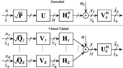
Figure 1: Processing for user $k$ in downlink and virtual uplink.

User $k$’s data streams are processed by the $M\times L_{k}$ transmit filter $\mathbf{U}_{k}=\left[\mathbf{u}_{k1},\ldots,\mathbf{u}_{kL_{k}}\right]$ before being transmitted over the $M$ antennas. Each $\mathbf{u}_{kj}$ is the precoder for stream $j$ of user $k$, and has unit power ($\|\mathbf{u}_{kj}\|_{2}=1$, where $\|\cdot\|_{2}$ is the Euclidean norm operator). These individual precoders together form the $M\times L$ global transmitter precoder matrix $\mathbf{U}=\left[\mathbf{U}_{1},\mathbf{U}_{2},\ldots,\mathbf{U}_{K}\right]$. Let $p_{kj}$ be the power allocated to stream $j$ of user $k$ and the downlink transmit power vector for user $k$ be $\mathbf{p}_{k}=\left[p_{k1},p_{k2},\ldots,p_{kL_{k}}\right]^{T}$, with $\mathbf{p}=\left[\mathbf{p}_{1}^{T},\ldots,\mathbf{p}_{K}^{T}\right]^{T}$. Define $\mathbf{P}_{k}=diag\{\mathbf{p}_{k}\}$ and $\mathbf{P}=diag\{\mathbf{p}\}$. The channel between the transmitter and user $k$ is assumed flat and is represented by the $N_{k}\times M$ matrix $\mathbf{H}_{k}^{H}$, where $(\cdot)^{H}$ indicates the conjugate transpose operator. The resulting $N\times M$ channel matrix is $\mathbf{H}^{H}$, with $\mathbf{H}=\left[\mathbf{H}_{1},\,\mathbf{H}_{2},\,\dots,\mathbf{H}_{K}\right].$ The transmitter is assumed to know the channel perfectly.

Based on this model, user $k$ receives a length $N_{k}$ vector

$$\mathbf{y}_{k}=\mathbf{H}_{k}^{H}\mathbf{U}\sqrt{\mathbf{P}}\mathbf{x}+\mathbf{n}_{k},$$ (1)

where $\mathbf{n}_{k}$ consists of the additive white Gaussian noise (AWGN) at the user’s receive antennas with power $\sigma^{2}$; that is, $\mathbb{E}\left[\mathbf{n}_{k}\mathbf{n}_{k}^{H}\right]=\sigma^{2}\mathbf{I}_{N_{k}}$, where $\mathbb{E}\left[\cdot\right]$ represents the expectation operator. To estimate its $L_{k}$ symbols $\mathbf{x}_{k}$, user $k$ processes $\mathbf{y}_{k}$ with its $L_{k}\times N_{k}$ decoder matrix $\mathbf{V}_{k}^{H}$ resulting in

$$\hat{\mathbf{x}}_{k}^{DL}=\mathbf{V}_{k}^{H}\mathbf{H}_{k}^{H}\mathbf{U}\sqrt{\mathbf{P}}\mathbf{x}+\mathbf{V}_{k}^{H}\mathbf{n}_{k},$$ (2)

where the superscript ^DL indicates the downlink.

The global receive filter $\mathbf{V}^{H}$ is a block diagonal decoder matrix of dimension $L\times N$, $\mathbf{V}=diag\left[\mathbf{V}_{1},\,\mathbf{V}_{2},\cdots,\mathbf{V}_{K}\right]$, where each $\mathbf{V}_{k}=\left[\mathbf{v}_{k1},\ldots,\mathbf{v}_{kL_{k}}\right]$.

We make use of the dual virtual uplink, also illustrated in Fig. 1, with the same channels between users and base station. Let the uplink transmit power vector for user $k$ be $\mathbf{q}_{k}=[q_{k1},q_{k2},\ldots,q_{kL_{k}}]^{T}$, with $\mathbf{q}=[\mathbf{q}_{1}^{T},\ldots,\mathbf{q}_{K}^{T}]^{T}$, and define $\mathbf{Q}_{k}=diag\{\mathbf{q}_{k}\}$ and $\mathbf{Q}=diag\{\mathbf{q}\}$. The transmit and receive filters for user $k$ become $\mathbf{V}_{k}$ and $\mathbf{U}_{k}^{H}$ respectively. As in the downlink, the precoder for the virtual uplink contains columns with unit norm; that is, $\|\mathbf{v}_{kj}\|_{2}=1$. The received vector at the base station and the estimated symbol vector for user $k$ are

$$\mathbf{y} = \sum_{i=1}^{K}\mathbf{H}_{i}\mathbf{V}_{i}\sqrt{\mathbf{Q}_{i}}\mathbf{x}_{i}+\mathbf{n},$$ (3)

$$\hat{\mathbf{x}}_{k}^{UL} = \sum_{i=1}^{K}\mathbf{U}_{k}^{H}\mathbf{H}_{i}\mathbf{V}_{i}\sqrt{\mathbf{Q}_{i}}\mathbf{x}_{i}+\mathbf{U}_{k}^{H}\mathbf{n}.$$ (4)

The noise term, $\mathbf{n}$, is again AWGN with $\mathbb{E}\left[\mathbf{n}\mathbf{n}^{H}\right]=\sigma^{2}\mathbf{I}_{M}$.

We assume that the modulated data symbols $\mathbf{x}$ are drawn from a PSK constellation where each data symbol $x_{i}$ has power $|x_{i}|^{2}=1$. Furthermore, the data symbols are independent so that $\mathbb{E}\left[\mathbf{x}\mathbf{x}^{H}\right]=\mathbf{I}_{L}$. Also, noise and data are independent such that $\mathbb{E}\left[\mathbf{x}_{i}\mathbf{n}^{H}\right]=\mathbf{0}$. Finally, we define a useful virtual uplink receive covariance matrix as

$$\mathbf{J} = \mathbb{E}\left[\mathbf{y}\mathbf{y}^{H}\right]=\sum_{k=1}^{K}\mathbf{H}_{k}\mathbf{V}_{k}\mathbf{Q}_{k}\mathbf{V}_{k}^{H}\mathbf{H}_{k}^{H}+\sigma^{2}\mathbf{I}_{M}$$ (5)

$$= \mathbf{HVQV}^{H}\mathbf{H}^{H}+\sigma^{2}\mathbf{I}_{M}.$$

III Product of Mean Squared Errors

Information theoretical approaches characterize the sum capacity of the multiuser MIMO downlink or broadcast channel (BC) by solving the sum capacity of the equivalent uplink multiple access channel (MAC) and applying a duality result [8, 20]. The resulting expression for the maximum sum rate in the $K$ user MAC is

$$R_{\mathrm{sum}} = \max_{\mathbf{\Sigma}_{k}}\log_{2}\det\left(\mathbf{I}+\frac{1}{\sigma^{2}}\sum_{k=1}^{K}\mathbf{H}_{k}\mathbf{\Sigma}_{k}\mathbf{H}_{k}^{H}\right)$$ (6)

$$\mathrm{s.t.}\quad\mathbf{\Sigma}_{k}\succeq\mathbf{0}\hskip 39.74872ptk=1,\ldots,K$$

$$\sum_{k=1}^{K}\mathrm{tr}\left[\mathbf{\Sigma}_{k}\right]\leq P_{\mathrm{max}},$$

where $\mathbf{\Sigma}_{k}\succeq\mathbf{0}$ indicates $\mathbf{\Sigma}_{k}$ is a positive semi-definite transmit covariance matrix for mobile user $k$ in the uplink. In this section, we approximate this sum rate in terms of each individual user’s data rate.

Consider the signal to interference plus noise ratio (SINR) for stream $j$ belonging to user $k$ under the multiuser virtual uplink model defined in Section II. Using (4) and finding the average received signal power ($\mathbb{E}\left[|\hat{x}_{kj}|^{2}\right]$) and interference-plus-noise power corresponding to all other data streams and AWGN, this stream achieves an SINR of

$$\gamma_{kj}^{UL} = \frac{\mathbf{u}_{kj}^{H}\mathbf{H}_{k}\mathbf{v}_{kj}q_{kj}\mathbf{v}_{kj}^{H}\mathbf{H}_{k}^{H}\mathbf{u}_{kj}}{\mathbf{u}_{kj}^{H}\mathbf{J}_{kj}\mathbf{u}_{kj}},$$ (7)

where $\mathbf{J}_{kj}\doteq\mathbf{J}-\mathbf{H}_{k}\mathbf{v}_{kj}q_{kj}\mathbf{v}_{kj}^{H}\mathbf{H}_{k}^{H}$ is the virtual uplink interference-plus-noise receive covariance matrix. We approximate the maximum rate for this stream as

$$R_{kj} \approx \log_{2}\left(1+\gamma_{kj}^{UL}\right).$$ (8)

Under the central limit theorem, the interference-plus-noise becomes Gaussian as the number of interfering streams increases, making the approximation progressively better.

The goal of this work is to maximize the sum data rate subject to constraints on the total available power. Using the approximation in (8), we formally state the optimization problem as:

$$\left(\mathbf{V},\mathbf{q}\right) = \arg\max_{\mathbf{V},\mathbf{q}}\sum_{k=1}^{K}\sum_{j=1}^{L_{k}}\log_{2}\left(1+\gamma_{kj}^{UL}\right)$$ (9)

$$\mathrm{s.t.}\quad\|\mathbf{v}_{kj}\|_{2}=1,\quad k=1,\ldots,K$$

$$\hskip 26.73953ptq_{kj}\geq 0,\hskip 23.12692ptj=1,\ldots,L_{k}$$

$$\|\mathbf{q}\|_{1}=\sum_{k=1}^{K}\sum_{j=1}^{L_{k}}q_{kj}\leq P_{\mathrm{max}},$$

where $\|\mathbf{q}\|_{1}$ is the 1-norm or the sum of all entries in $\mathbf{q}$.

We can see from (7) that the optimum linear receiver $\mathbf{u}_{kj}$ does not depend on any other columns of $\mathbf{U}$; furthermore, it is the solution to the generalized eigenproblem

$$\mathbf{u}_{kj}^{\mathrm{opt}} = \hat{e}_{\max}\left(\mathbf{H}_{k}\mathbf{v}_{kj}q_{kj}\mathbf{v}_{kj}^{H}\mathbf{H}_{k}^{H},\mathbf{J}_{kj}\right),$$ (10)

where $\hat{e}_{\max}(\mathbf{A},\mathbf{B})$ is the unit norm eigenvector $\mathbf{x}$ corresponding to the largest eigenvalue $\lambda$ in the generalized eigenproblem $\mathbf{Ax}~{}=~{}\lambda\mathbf{Bx}$. Within a normalizing factor, this solution is equivalent to the MMSE receiver:

$$\mathbf{u}_{kj}^{\mathrm{opt}} = \mathbf{J}^{-1}\mathbf{H}_{k}\mathbf{v}_{kj}\sqrt{q_{kj}}.$$ (11)

When using linear decoding with this MMSE receiver, the MSE matrix for the virtual uplink is

$$\mathbf{E} = \mathbb{E}\left[\left(\hat{\mathbf{x}}-\mathbf{x}\right)\left(\hat{\mathbf{x}}-\mathbf{x}\right)^{H}\right]$$ (12)

$$= \mathbf{I}_{L}-\sqrt{\mathbf{Q}}\mathbf{V}^{H}\mathbf{H}^{H}\mathbf{J}^{-1}\mathbf{HV}\sqrt{\mathbf{Q}},$$

which follows from (11) and the system model assumptions stated in Section II. Thus, the mean squared error for user $k$’s $j^{\mathrm{th}}$ stream is

$$\epsilon_{kj} = 1-q_{kj}\mathbf{v}_{kj}^{H}\mathbf{H}_{k}^{H}\mathbf{J}^{-1}\mathbf{H}_{k}\mathbf{v}_{kj}.$$ (13)

Now consider another optimization problem, minimizing the product of mean squared errors (PMSE) under a sum power constraint,

$$\left(\mathbf{V},\mathbf{q}\right) = \arg\min_{\mathbf{V},\mathbf{q}}\prod_{k=1}^{K}\prod_{j=1}^{L_{k}}\epsilon_{kj}$$ (14)

$$\mathrm{s.t.}\quad\|\mathbf{v}_{kj}\|_{2}=1,\quad k=1,\ldots,K$$

$$\hskip 26.73953ptq_{kj}\geq 0,\hskip 23.12692ptj=1,\ldots,L_{k}$$

$$\|\mathbf{q}\|_{1}=\sum_{k=1}^{K}\sum_{j=1}^{L_{k}}q_{kj}\leq P_{\mathrm{max}}.$$

Theorem 1

Under linear MMSE decoding at the base station, the optimization problems defined by (9) and (14) are equivalent problems.

Proof:

Define the argument of the log term from (8) as $\alpha_{kj}\doteq 1+\gamma_{kj}^{UL}$. Using (7), we can rewrite $\alpha_{kj}$ as

$$\alpha_{kj} = \frac{\mathbf{u}_{kj}^{H}\mathbf{J}\mathbf{u}_{kj}}{\mathbf{u}_{kj}^{H}\mathbf{J}\mathbf{u}_{kj}-\mathbf{u}_{kj}^{H}\mathbf{H}_{k}\mathbf{v}_{kj}q_{kj}\mathbf{v}_{kj}^{H}\mathbf{H}_{k}^{H}\mathbf{u}_{kj}}.$$ (15)

It follows that by using the MMSE receiver from (11),

$$\frac{1}{\alpha_{kj}} = 1-\frac{\mathbf{u}_{kj}^{H}\mathbf{H}_{k}\mathbf{v}_{kj}q_{kj}\mathbf{v}_{kj}^{H}\mathbf{H}_{k}^{H}\mathbf{u}_{kj}}{\mathbf{u}_{kj}^{H}\mathbf{J}\mathbf{u}_{kj}}$$ (16)

$$= 1-\frac{\left(q_{kj}\mathbf{v}_{kj}^{H}\mathbf{H}_{k}^{H}\mathbf{J}^{-1}\mathbf{H}_{k}\mathbf{v}_{kj}\right)^{2}}{q_{kj}\mathbf{v}_{kj}^{H}\mathbf{H}_{k}^{H}\mathbf{J}^{-1}\mathbf{H}_{k}\mathbf{v}_{kj}}$$

$$= 1-q_{kj}\mathbf{v}_{kj}^{H}\mathbf{H}_{k}^{H}\mathbf{J}^{-1}\mathbf{H}_{k}\mathbf{v}_{kj}=\epsilon_{kj}.$$

Thus, under linear MMSE decoding, the MSE and SINR for stream $j$ belonging to user $k$ are related as

$$\epsilon_{kj}=\frac{1}{1+\gamma_{kj}^{UL}}.$$ (17)

This relationship is similar to one shown for MMSE detection in CDMA systems [21]. By applying (17) to (9), we see that

$$\sum_{k=1}^{K}\sum_{j=1}^{L_{k}}\log_{2}\left(1+\gamma_{kj}^{UL}\right)=-\log_{2}\left(\prod_{k=1}^{K}\prod_{j=1}^{L_{k}}\epsilon_{kj}\right).$$ (18)

Since the constraints on $\mathbf{v}_{kj}$ and $q_{kj}$ are identical in (9) and (14), the problem of maximizing sum rate in (9) is therefore equivalent to minimizing the PMSE in (14). ∎

IV PMSE Minimization Algorithm

With the motivation of Section III in mind, we now develop an algorithm to minimize the product of mean squared errors. The algorithm draws on previous work in minimizing the sum MSE [3, 4]. It operates by iteratively obtaining the downlink precoder matrix $\mathbf{U}$ and power allocations $\mathbf{p}$ and the virtual uplink precoder matrix $\mathbf{V}$ and power allocations $\mathbf{q}$. Each step minimizes the objective function by modifying one of these four variables while leaving the remaining three fixed.

IV-A Downlink Precoder

For a fixed set of virtual uplink precoders $\mathbf{V}_{k}$ and power allocation $\mathbf{q}$, the optimum virtual uplink decoder $\mathbf{U}$ is defined by (11). Each $\epsilon_{kj}$ is minimized individually by this MMSE receiver, thereby also minimizing the product of MSEs. This $\mathbf{U}$ is normalized and used as the downlink precoder.

IV-B Downlink Power Allocation

The MSE duality derived in [3, 4] states that all achievable MSEs in the uplink for a given $\mathbf{U}$, $\mathbf{V}$, and $\mathbf{q}$ (with sum power constraint $\|\mathbf{q}\|_{1}\leq P_{\max}$), can also be achieved by a power allocation $\mathbf{p}$ in the downlink where $\|\mathbf{p}\|_{1}\leq P_{\max}$.

In order to calculate the power allocation $\mathbf{p}$, we apply the following result from [4]:

$$\mathbf{p}=\sigma^{2}(\mathbf{D}^{-1}-\mathbf{\Psi})^{-1}\mathbf{1},$$ (19)

where $\mathbf{\Psi}$ is the $L\times L$ cross coupling matrix defined as

$$[\mathbf{\Psi}]_{ij}=\left\{\begin{array}[]{ll}|\mathbf{\tilde{h}}_{i}^{H}\mathbf{u}_{j}|^{2}=|\mathbf{u}_{j}^{H}\mathbf{\tilde{h}}_{i}|^{2}&\textrm{${i}\neq{j}$}\\ 0&\textrm{$i=j$}\end{array}\right.,$$ (22)

$$\mathbf{D}=\mathrm{diag}\left\{\frac{\gamma_{11}^{UL}}{|\mathbf{v}_{11}^{H}\mathbf{H}_{1}^{H}\mathbf{u}_{11}|^{2}},\dots,\frac{\gamma_{KL_{K}}^{UL}}{|\mathbf{v}_{KL_{K}}^{H}\mathbf{H}_{K}^{H}\mathbf{u}_{KL_{K}}|^{2}}\right\},$$

where $\mathbf{\tilde{H}}=\mathbf{H}\mathbf{V}=[\mathbf{\tilde{h}}_{1},\ldots,\mathbf{\tilde{h}}_{L}]$, $\mathbf{U}=[\mathbf{u}_{1},\ldots,\mathbf{u}_{L}]$, and $\mathbf{1}$ is the all-ones vector of the required dimension.

IV-C Virtual Uplink Precoder

Given a fixed $\mathbf{U}$ and $\mathbf{p}$, the optimal decoders $\mathbf{V}_{k}$ are the MMSE receivers:

$$\mathbf{V}_{k}=\mathbf{J}_{k}^{-1}\mathbf{H}_{k}^{H}\mathbf{U}_{k}\sqrt{\mathbf{P}_{k}}.$$ (23)

In this equation, $\mathbf{J}_{k}\doteq\mathbf{H}_{k}^{H}\mathbf{UPU}^{H}\mathbf{H}_{k}+\sigma^{2}\mathbf{I}_{N_{k}}$ is the receive covariance matrix for user $k$. The optimum virtual uplink precoders are then the normalized columns of $\mathbf{V}_{k}$.

IV-D Virtual Uplink Power Allocation

The power allocation problem on the virtual uplink solves (14) with a fixed matrix $\mathbf{V}$. In the minimization of sum MSE, the corresponding step is a convex optimization problem [4]. Unfortunately, it is well accepted that the power allocation subproblem in PMSE minimization (or equivalently, in sum rate maximization) is non-convex [14, 16, 17].

We thus employ numerical techniques to solve the power allocation subproblem, and use sequential quadratic programming (SQP) [22] to minimize the PMSE. SQP solves successive approximations of a constrained optimization problem and is guaranteed to converge to the optimum value for convex problems; however, in the case of this non-convex optimization problem, SQP can only guarantee convergence to a local minimum. We note that a similar approach was proposed in [17], where iterations of the the sum rate maximization problem are solved by local approximations of the non-convex sum-rate function as a (convex) geometric program [23].

In summary, the PMSE minimization algorithm, motivated by a need to maximize sum data rate, follows the same steps as the minimization of the SMSE. The iterative algorithm keeps three of four parameters ($\mathbf{U},\mathbf{p},\mathbf{V},\mathbf{q}$) fixed at each step and obtains the optimal value of the fourth. Convergence of the overall algorithm to a local minimum is guaranteed since the PMSE objective function is non-increasing at each of the four parameter update steps. Termination of the algorithm is determined by the selection of the convergence threshold $\epsilon$.

While neither the overall problem (14) nor the power allocation subproblem are believed to be convex, simulations suggest that changing the initialization point has a minimal impact on the final solution; however, initialization with the $\mathbf{U}$ and $\mathbf{p}$ found using the SMSE algorithm in [4] appears to reduce the number of iterations required for convergence. A summary of our proposed algorithm can be found in Table I.

TABLE I: Iterative PMSE minimization algorithm

Iteration:

1-   Downlink Precoder

$\mathbf{\tilde{U}}_{k}=\mathbf{J}^{-1}\mathbf{H}_{k}^{H}\mathbf{V}_{k}\sqrt{\mathbf{Q}_{k}}$,   $\mathbf{u}_{kj}=\frac{\mathbf{\tilde{u}}_{kj}}{\|\mathbf{\tilde{u}}_{kj}\|_{2}}$

2-   Downlink Power Allocation via MSE duality

$\mathbf{p}=\sigma^{2}(\mathbf{D}^{-1}-\mathbf{\Psi})^{-1}\mathbf{1}$

3-   Virtual Uplink Precoder

$\mathbf{\tilde{V}}_{k}=\mathbf{J}^{-1}_{k}\mathbf{H}_{k}^{H}\mathbf{U}_{k}\sqrt{\mathbf{P}_{k}}$,   $\mathbf{v}_{kj}=\frac{\mathbf{\tilde{v}}_{kj}}{\|\mathbf{\tilde{v}}_{kj}\|_{2}}$

4-   Virtual Uplink Power Allocation

$\mathbf{q}=\arg\min_{\mathbf{q}}\prod_{k=1}^{K}\prod_{j=1}^{L_{k}}\epsilon_{kj}$, s.t. $q_{kj}\geq 0$, $\|\mathbf{q}\|_{1}\leq P_{\max}$

5-   Repeat 1–4 until $\left[\mathrm{PMSE}_{\mathrm{old}}-\mathrm{PMSE}_{\mathrm{new}}\right]/\mathrm{PMSE}_{\mathrm{old}}<\epsilon$

V Numerical Examples

In this section, we present simulation results to illustrate the performance of the proposed algorithms. In all cases, the fading channel is modelled as flat and Rayleigh using a channel matrix $\mathbf{H}$ composed of independent and identically distributed samples of a complex Gaussian process with zero mean and unit variance. The examples use a maximum transmit power of $P_{\max}=1$; SNR is controlled by varying the receiver noise power $\sigma^{2}$. The transmitter is assumed to have perfect knowledge of the channel matrix $\mathbf{H}$.

V-A Theoretical Performance

First, we examine the information theoretical performance of the PMSE algorithm proposed in Section IV. That is, we consider the spectral efficiency (measured in bps/Hz) that could be achieved under ideal transmission by drawing transmit symbols from a Gaussian codebook. Figure 2 illustrates how the proposed scheme performs when compared to the sum capacity for the broadcast channel (i.e. using dirty paper coding (DPC) [11]) and to traditional linear precoding methods based on channel orthogonalization (i.e. block diagonalization (BD) and zero forcing (ZF) [13]). This simulation models a $K=2$ user system with $M=4$ transmit antennas and $N_{k}=2$ or $N_{k}=4$ receive antennas per user. The plot is generated using $30000$ channel realizations, with $5000$ data symbols per channel realization, and the convergence threshold for the PMSE algorithm is set as $\epsilon=10^{-6}$.

In Fig. 2, we see a slight divergence in the performance of the PMSE algorithm from the theoretical DPC bound at higher SNR. This drop in spectral efficiency may be caused by the non-convexity of the optimization problem, or it may suggest a fundamental gap between the optimal DPC bound and the achievable sum capacity under linear precoding. Nonetheless, the PMSE algorithm still maintains a higher spectral efficiency than the orthogonalization based schemes for $N_{k}=2$. Furthermore, the gap between the DPC bound and the PMSE precoder is only 0.6 dB for $N_{k}=4$, where BD and ZF schemes can not be applied due to constraints on the number of antennas.

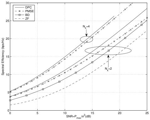
Figure 2: PMSE vs. DPC and orthogonalization–based methods

V-B Performance Using Practical Modulation

The precoder and decoder design algorithm in Section IV is derived independently of modulation depth, based on the assumption that transmitted symbols originate from a unit-energy PSK constellation. In this section, we consider two approaches in selecting the modulation scheme to maximize data rate.

The naive approach selects the largest PSK constellation of $b_{kj}$ bits per stream that satisfies a maximum bit error rate (BER) requirement of $\beta_{kj}$. The satisfaction of this constraint is determined using a closed form BER approximation [24],

$$\mathrm{BER}_{\mathrm{PSK}}(\gamma)\approx c_{1}\exp\left(\frac{-c_{2}\gamma}{2^{c_{3}b}-c_{4}}\right).$$ (24)

We apply the least aggressive of the bounds proposed in [24] by using the values $c_{1}=0.25$,$c_{2}=8$,$c_{3}=1.94$, and $c_{4}=0$. We note that this approximation only holds for $b\geq 2$; as such, the following exact expression should be used for BPSK:

$$\mathrm{BER}_{\mathrm{BPSK}}(\gamma)\approx\frac{1}{2}\mathrm{erfc}\left(\sqrt{\gamma}\right).$$ (25)

The BPSK expression can be used as a test of feasibility for the specified BER target; if the resulting BER under BPSK modulation is higher than $\beta_{kj}$, then we have two options: either declare the BER target infeasible, or transmit using the lowest modulation depth available (i.e. BPSK). In this work, we have elected to transmit using BPSK whenever the PMSE stage has allocated power to the data stream. Future work may consider either partial or complete non-transmission to implement power saving while strictly achieving the desired BER target.

The naive approach is quite conservative in that there may be a large gap between the BER requirement and BER achieved for each channel realization. We suggest a probabilistic bit allocation scheme that switches between $b_{kj}$ bits (as determined by the naive approach) and $b_{kj}+1$ bits with probability $p_{kj}=\left[\beta_{kj}-\mathrm{BER}_{b_{kj}}\right]/\left[\mathrm{BER}_{b_{kj}+1}-\mathrm{BER}_{b_{kj}}\right]$. This modulation strategy may not be appropriate for systems requiring instantaneous satisfaction of BER constraints; however, the probabilistic method will still achieve the desired BER in the long-term average over channel realizations.

Figure 3 shows the sum rate achieved in the same system configuration as described above ($K~{}=~{}2$, $M~{}=~{}4$, $N_{k}~{}=~{}2$) with the additional required specification of $L_{k}=2$ data streams per user and a target bit error rate of $\beta_{kj}=10^{-2}$. The plot illustrates the average number of bits per transmission for user 1; due to symmetry, the corresponding plot for user 2 is identical. Note that in contrast to Fig. 2 (which shows the sum capacity under ideal Gaussian coding), the sum rate in Fig. 3 is the average number of bits transmitted in each realization using symbols from a PSK constellation.

In Fig. 3, we also consider using the naive PSK modulation scheme for the PMSE precoder and the SMSE precoder designed in [4]. Examination of this plot reveals that using the PMSE criterion is justified at practical SNR values with improvements of approximately one bit per transmission near 15 dB. Furthermore, using the probabilistic modulation scheme (designated “PMSE-P”) yields an additional improvement of more than half a bit per transmission across all SNR values.

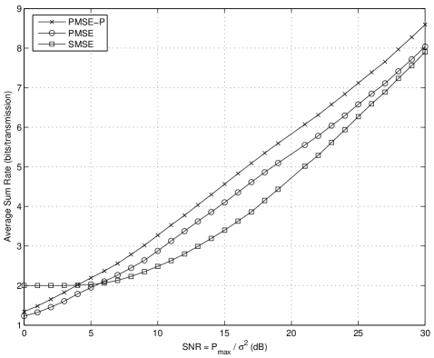
Figure 3: Sum rate vs. SNR for user 1

In Fig. 4, we plot average BER versus SNR for the same system configuration as in Fig. 3. This plot illustrates how the naive bit allocation algorithm attempts to achieve the target BER of $10^{-2}$ for all data streams under PMSE, but also overshoots the target, converging to a BER of approximately $5\times 10^{-4}$. This can be attributed to the looseness of the BER bound, as discussed above. In contrast, the probabilistic rate allocation algorithm not only increases the rate, as shown in Fig. 3, but also converges to a BER that is much closer to the desired target BER. The remaining gap between the actual BER achieved and the target BER can be attributed to looseness in the approximations of (24) and (25).

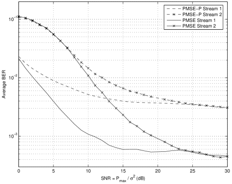
Figure 4: BER vs. SNR for user 1

VI Conclusions

In this paper, we have considered the problem of designing an iterative method for maximizing bit rates in the multiuser MIMO downlink. Previous work in the multiuser downlink has focused largely on added reliability (minimizing SMSE), and not on maximizing the data rate. We have designed a solution for a general MIMO system, where the number of users, base station antennas, mobile antennas, and streams transmitted are only constrained by resolvability of the data symbols. Our proposed solution uses the SINR duality results from previous work in minimizing SMSE. The product of the MSEs for all streams is minimized under a sum power constraint; this is achieved by employing a known uplink-downlink duality of MSEs. We also presented an adaptive modulation scheme to realize these gains in rate in a practical system. The resulting SINR on each data stream is then used to select an appropriate PSK constellation. Simulations verify that significantly increased data rates can be achieved while meeting given BER constraints.

References

- [1] A. J. Tenenbaum and R. S. Adve, “Joint multiuser transmit-receive optimization using linear processing,” in Proc. IEEE Internat. Conf. on Communications (ICC 04), vol. 1, Paris, France, Jun. 2004, pp. 588–592.
- [2] S. Shi and M. Schubert, “MMSE transmit optimization for multi-user multi-antenna systems,” in Proc. IEEE Internat. Conf. on Acoustics, Speech, and Signal Proc. (ICASSP 05), Philadelphia, PA, Mar. 2005.
- [3] M. Schubert, S. Shi, E. A. Jorswieck, and H. Boche, “Downlink sum-MSE transceiver optimization for linear multi-user MIMO systems,” in Proc. Asilomar Conf. on Signals, Systems and Computers, Monterey, CA, Sep. 2005, pp. 1424–1428.
- [4] A. M. Khachan, A. J. Tenenbaum, and R. S. Adve, “Linear processing for the downlink in multiuser MIMO systems with multiple data streams,” in Proc. IEEE Internat. Conf. on Communications (ICC 06), Istanbul, Turkey, Jun. 2006.
- [5] M. Schubert and H. Boche, “Solution of the multiuser downlink beamforming problem with individual SINR constraints,” IEEE Trans. Veh. Technol., vol. 53, no. 1, pp. 18–28, Jan. 2004.
- [6] A. Mezghani, M. Joham, R. Hunger, and W. Utschick, “Transceiver design for multi-user MIMO systems,” in Proc. ITG/IEEE Workshop on Smart Antennas, Ulm, Germany, Mar. 2006.
- [7] H. Boche, M. Schubert, and E. A. Jorswieck, “Throughput maximization for the multiuser MIMO broadcast channel,” in Proc. IEEE Internat. Conf. on Acoustics, Speech, and Signal Proc. (ICASSP 03), vol. 4, Hong Kong, Apr. 2003, pp. 808–811.
- [8] P. Viswanath and D. N. C. Tse, “Sum capacity of the vector Gaussian broadcast channel and uplink-downlink duality,” IEEE Trans. Inf. Theory, vol. 49, no. 8, pp. 1912–1921, Aug. 2003.
- [9] W. Yu and J. M. Cioffi, “Sum capacity of Gaussian vector broadcast channels,” IEEE Trans. Inf. Theory, vol. 50, no. 9, pp. 1875–1892, Sep. 2004.
- [10] N. Jindal, W. Rhee, S. Vishwanath, S. A. Jafar, and A. Goldsmith, “Sum power iterative water-filling for multiple-antenna Gaussian broadcast channels,” IEEE Trans. Inf. Theory, vol. 51, no. 4, pp. 1570–1580, Apr. 2005.
- [11] M. Costa, “Writing on dirty paper,” IEEE Trans. Inf. Theory, vol. 29, no. 3, pp. 439–441, May 1983.
- [12] C. Windpassinger, R. F. H. Fischer, T. Vencel, and J. B. Huber, “Precoding in multiantenna and multiuser communications,” IEEE Trans. Wireless Commun., vol. 3, no. 4, pp. 1305–1336, Jul. 2004.
- [13] J. Lee and N. Jindal, “Dirty paper coding vs. linear precoding for MIMO broadcast channels,” in Proc. Asilomar IEEE Conf. on Signals, Systems, and Computers, Asilomar, CA, Oct. 2006, pp. 779–783.
- [14] D. A. Schmidt, M. Joham, R. Hunger, and W. Utschick, “Near maximum sum-rate non-zero-forcing linear precoding with successive user selection,” in Proc. Asilomar Conf. on Signals, Systems and Computers, October 2006, pp. 2092–2096.
- [15] M. Stojnic, H. Vikalo, and B. Hassibi, “Rate maximization in multi-antenna broadcast chanels with linear preprocessing,” IEEE Trans. Wireless Commun., vol. 5, no. 9, pp. 2338–2342, September 2006.
- [16] F. Boccardi, F. Tosato, and G. Caire, “Precoding schemes for the MIMO–GBC,” in Proc. Int. Zurich Seminar on Communications, February 2006, pp. 10–13.
- [17] M. Codreanu, A. Tölli, M. Juntti, and M. Latva-aho, “Joint design of Tx-Rx beamformers in MIMO downlink channel,” IEEE Trans. Signal Process., vol. 55, no. 9, pp. 4639–4655, September 2007.
- [18] D. P. Palomar, J. M. Cioffi, and M. A. Lagunas, “Joint Tx-Rx beamforming design for multicarrier MIMO channels: A unified framework for convex optimization,” IEEE Trans. Signal Process., vol. 51, no. 9, pp. 2381–2401, Sep. 2003.
- [19] D. Guo, S. Shamai, and S. Verdu, “Mutual information and minimum mean-square error in Gaussian channels,” IEEE Trans. Inf. Theory, vol. 51, no. 4, pp. 1261–1282, Apr. 2005.
- [20] S. Vishwanath, N. Jindal, and A. Goldsmith, “Duality, achievable rates, and sum-rate capacity of Gaussian MIMO broadcast channels,” IEEE Trans. Inf. Theory, vol. 49, no. 10, pp. 2658–2668, Oct. 2003.
- [21] U. Madhow and M. L. Honig, “MMSE interference suppression for direct-sequence spread-spectrum CDMA,” IEEE Trans. Commun., vol. 42, no. 12, pp. 3178–3188, Dec. 1994.
- [22] P. T. Boggs and J. W. Tolle, “Sequential quadratic programming,” in Acta Numerica. Cambridge University Press, 1995, pp. 1–51.
- [23] S. Boyd and L. Vandenberghe, Convex Optimization. Cambridge University Press, 2004.
- [24] S. T. Chung and A. J. Goldsmith, “Degrees of freedom in adaptive modulation: a unified view,” IEEE Trans. Commun., vol. 49, no. 9, pp. 1561–1571, Sep. 2001.