Bright Giant Pulses from the Crab Nebula Pulsar: Statistical Properties, Pulse Broadening and Scattering due to the Nebula

Abstract

We report observations of Crab giant pulses made with the Australia Telescope Compact Array and a baseband recorder system, made simultaneously at two frequencies, 1300 and 1470 MHz. These observations were sensitive to pulses with amplitudes $\scriptscriptstyle\stackrel{{\scriptstyle>}}{{\sim}}$ 3 kJy and widths $\scriptscriptstyle\stackrel{{\scriptstyle>}}{{\sim}}$ 0.5 $\mu$s. Our analysis led to the detection of more than 700 such bright giant pulses over 3 hours, and using this large sample we investigate their amplitude, width, arrival time and energy distributions. The brightest pulse detected in our data has a peak amplitude of $\sim$ 45 kJy and a width of $\sim$ 0.5 $\mu$s, and therefore an inferred brightness temperature of $\sim 10^{35}$ K. The duration of giant-pulse emission is typically $\sim$1 $\mu$s, however it can also be as long as 10 $\mu$s. The pulse shape at a high time resolution (128 ns) shows rich diversity and complexity in structure and is marked by an unusually low degree of scattering. We discuss possible implications for scattering due to the nebula, and for underlying structures and electron densities.

1 Introduction

The Crab Nebula pulsar B0531+21 is well known for its emission of giant radio pulses, and was originally discovered through the detection of such pulses (Staelin & Reifenstein, 1968). These sporadic, large-amplitude and short-duration bursts can be hundreds or thousands of times more energetic than regular pulses (e.g. Lundgren et al., 1995), and they remain one of the most enigmatic aspects of pulsar radio emission. While several other pulsars are now known to emit giant pulses (e.g. Cognard et al., 1996; Johnston et al., 2004; Knight et al., 2006), only 3 objects, viz. the Crab and the millisecond pulsars B1937+21 and J1823–3021A, generate giant pulses numerous enough to allow detailed studies of their characteristics.

Observations so far have unravelled several fundamental properties of giant pulse emission. It is now fairly well established that the fluctuations in their amplitudes are due to changes in the coherence of the radio emission (Lundgren et al., 1995), and that they are superpositions of extremely narrow nanosecond structures (Hankins et al., 2003). Observations also suggest that the emission is broadband, extending over several hundreds of MHz (Sallmen et al., 1999; Popov et al., 2006). Another important characteristic of giant pulses is their tendency to originate in a very narrow phase window of regular radio emission; and for the Crab, these windows even coincide with the phases of the high-energy (from infrared to $\gamma$-ray) emission (Moffett & Hankins, 1996). Finally, the distribution of giant pulse energies is known to follow a power-law form (Argyle & Gower, 1972; Lundgren et al., 1995), much in contrast to the Gaussian or exponential distribution typical of regular pulses (e.g. Hesse & Wielebinski, 1974).

Of all the giant-pulse–emitting pulsars, the Crab is the most well-studied. It is known to emit pulses as energetic as $\sim 10^{4}$ times regular pulses (Cordes et al., 2004) and shows structures persisting down to 2 ns, with inferred brightness temperatures as high as $10^{37}$ K (Hankins et al., 2003). Given such extreme short durations, giant pulses are best studied using data from baseband observations. Such data allow coherent dedispersion of voltage samples to remove the deleterious effect of interstellar dispersion, thereby yielding more accurate descriptions of pulse structure, shape and amplitude. However, the bulk of the observational studies of the Crab until the early 2000s were carried out using traditional filterbank or spectrometer data, due to limitations of data throughput and computing. With the advent of wide-bandwidth recorders and affordable high-power computing, these limitations are being gradually overcome. As a result, baseband observations are increasingly employed in giant pulse studies (e.g. Soglasnov et al., 2004; Popov & Stappers, 2007).

In this paper, we report our observations of Crab giant pulses made using the Australia Telescope Compact Array (ATCA) and the baseband recorder recently developed for the Australian Long Baseline Array. We detected over 700 giant pulses with amplitudes $\scriptscriptstyle\stackrel{{\scriptstyle>}}{{\sim}}$ 3 kJy and widths $\sim$0.5 to 10 $\mu$s, and using this large sample we investigate aspects such as the pulse amplitude, width, arrival time and energy distributions, as well as details of the pulse structure and shape. Our observations show a much lower degree of scattering than reported before and we discuss possible implications for scattering due to the nebula.

2 Observations and Data Processing

2.1 Observations with the ATCA

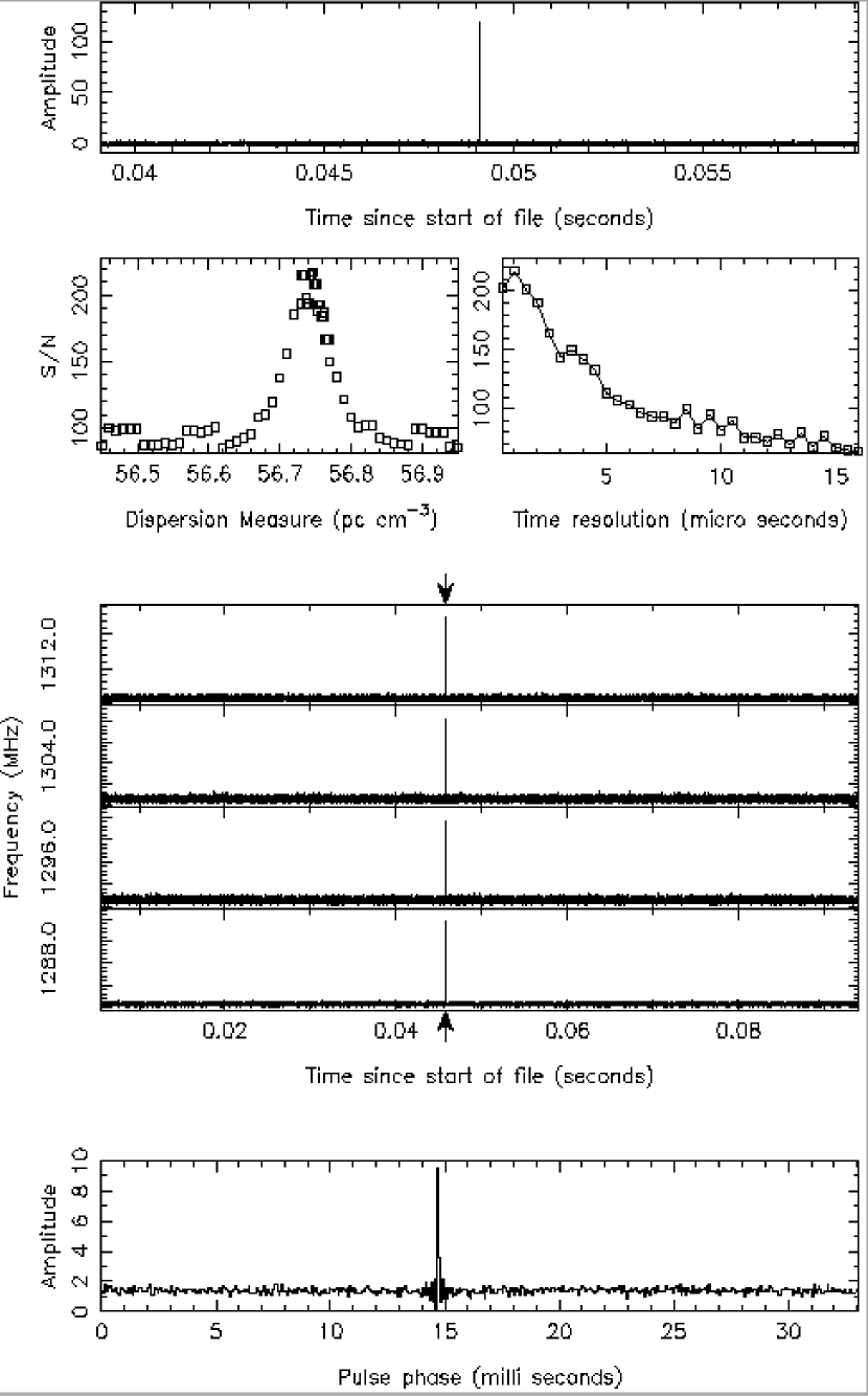
Figure 1: Example plots illustrating our giant pulse detection. Top: Dedispersed time series of a short data segment around the giant pulse. Middle panels: Diagnostic plots from the giant pulse search; plots of signal-to-noise ratio vs trial dispersion measure and time resolution, and dedispersed pulses over four 8-MHz sub-bands of the 32 MHz recorder bandwidth. Bottom: The dedispersed pulse over a time window of 33 ms (i.e. one rotation period).

Observations of the Crab pulsar were made in January 2006. Although the array offers maximal sensitivity for pulsar observations in its tied-array mode, our observing set-up was designed also to meet certain technical goals in addition to pulsar observations, and offered a sensitivity equivalent to that of a single ATCA antenna. In this set-up, the array was configured to record two independent IF (intermediate frequency) signals, each 32 MHz in bandwidth, from a single antenna. At the antenna, two 64-MHz bands were Nyquist-sampled at 128 MHz, with four bits per voltage sample, for two orthogonal linear polarisations. These data were converted to circular polarisations by inserting a $90^{\circ}$ phase shifter in the signal path. The signals were then digitally filtered to provide two-bit sampled voltage time series for the 32 MHz bandwidth. This results in an aggregate data rate of 512 megabits per second. The system provided flexibility to record either two separate frequency bands from a single antenna, or two identical frequency bands from two different antennas. The pulsar observations were made over a total duration of 3 hours; the first half of which used two 32-MHz bands (dual polarisation) centred at frequencies 1300 and 1470 MHz, while the remaining half used two identical frequency bands centred at 1300 MHz from two different antennas. This accumulated a total data volume of 5.5 terabytes, but split into a large number of short blocks of 10 s duration each to facilitate further analysis and processing. The data were stored onto disks for offline processing and all processing operations, such as coherent dedispersion, detection and search for giant pulses, were performed at the Swinburne University of Technology Supercomputing Facility.

2.2 Data Decoding and Dedispersion

Data samples from both the polarisation channels of the two IF bands were organised into a single data stream while recording, and were subsequently decoded into separate IF data streams before de-dispersion and further processing. As our processing software is designed to handle a single data stream at a given time, this meant two separate passes for processing each short block of data. The unpacked data from this stage were then dedispersed using the coherent dispersion removal technique originally developed by Hankins (1971). The procedures we have adopted are similar to those described in Knight et al. (2006) and Bhat et al. (2007). Voltage samples are first Fourier transformed to the frequency domain and the spectra are divided into a series of sub-bands. Each sub-band is then multiplied by an inverse response filter (kernel) for the ISM (e.g. Hankins & Rickett, 1975; van Straten, 2003), and then Fourier transformed back to the time domain to construct a time series with a time resolution coarser than the original data. By splitting the input signal into several sub-bands (four in our case), the dispersive smearing is essentially reduced to that of an individual sub-band. This also means the procedure uses shorter transforms than single-channel coherent dedispersion and is consequently a more computationally efficient method. The coherent filterbank stream data obtained in this manner are then square-law detected, corrected for dispersive delays between the sub-bands, and summed in polarisation to construct a single coherently dedispersed time series for the entire band.

2.3 Search for Giant Pulses

Following the procedures of decoding and dedispersion, we performed a rigorous search for giant pulses within each 10 s block of data. Our pulse detection procedure involved progressive smoothing of time series with matched filters of widths ranging from 0.5 to 16 $\mu$s in steps of 0.5 $\mu$s, and identifying the intensity samples that exceed a set threshold (e.g. 12$\sigma$ for the 0.5 $\mu$s smoothing time). In addition to performing dedispersion at the Crab’s nominal DM of 56.75 ${\rm pc\ cm^{-3}}$ , we also performed this procedure over a large number of adjacent DM values (typically over a DM range $\approx$ 0.5 ${\rm pc\ cm^{-3}}$ , in steps of 0.001 ${\rm pc\ cm^{-3}}$ ). For each DM and the matched filter width, we computed the signal-to-noise ratio (S/N) of the pulse amplitude over a short stretch of data centred at the pulse maximum. From this analysis, diagnostic plots are generated for each candidate giant pulse as shown in Fig. 1. These plots are subjected to a careful human scrutiny to discriminate real giant pulses from spurious signals.

2.4 Summary of Detections

We adopted a rather conservative threshold of 12$\sigma$ in order to account for possible departures of noise statistics from those expected of pure white noise and also to limit the number of candidate signals to a reasonable number. With this threshold and the 0.5 $\mu$s final time resolution ($\Delta t$) employed in our analysis, a pulse will need to be $\scriptscriptstyle\stackrel{{\scriptstyle>}}{{\sim}}$ 3 kJy in amplitude to enable a clear detection (see § 2.5). We detected 706 giant pulses from our 3-hr long observation, of which 413 are from the first half of observations that were made simultaneously at 1300 and 1470 MHz. However, only 70% of these 413 were detected in both frequency bands. This fraction is similar to that reported by Sallmen et al. (1999) from their observations at 600 and 1400 MHz, although quite different fractions have been reported from observations at widely separated frequencies (Kostyuk et al., 2003) and at lower frequencies (Popov et al., 2006). This probably suggests that not all pulses are entirely broadband, a characteristic presumably intrinsic to the giant-pulse emission phenomenon. Our sample includes pulses with widths ranging from 0.5 to 10 $\mu$s. Given $\Delta t$ = 0.5 $\mu$s, any shorter-duration pulses that may be present in our data will be smoothed to an effective resolution of 0.5 or 1 $\mu$s. Moreover, pulses broader than 10 $\mu$s are likely to be weaker than our detection threshold. The strongest pulse in our observations is 0.5 $\mu$s in duration and has a S/N of 217.

2.5 System Sensitivity and Flux Calibration

The Crab Nebula is a fairly bright and extended source in the radio sky, with a flux density of $\sim$955$\,\nu^{-0.27}$ Jy (Bietenholz et al. (1997); where $\nu$ is the frequency in GHz) and a characteristic diameter of $\sim$5^′.5. Thus, in general, there will be a significant contribution from the nebula to the system noise ($S$), depending on the frequency of observation and the coverage of the nebula within the telescope beam. However, in our case, the problem is much simplified as the nebula is unresolved by a single antenna of the array (half-power beam width $\approx$ $33^{\prime}$ at our observing frequencies). In fact, the entire nebular region occupies only a small fraction ($\approx$ 3%) of the beam solid angle. Measurements made in parallel with the observations yield system temperatures (${\rm T_{sys}}$ ) of $114\,\pm\,3$ and $103\,\pm\,2$ K respectively at 1300 and 1470 MHz. Thus, assuming a nominal gain (G) of $\approx$ 0.1 ${\rm K\,Jy^{-1}}$ for a single ATCA antenna at L-band, these measurements translate to system equivalent flux densities (${\rm S_{sys}}$ =${\rm T_{sys}}$ /G) of 1140 and 1030 Jy respectively at 1300 and 1470 MHz. Scaling for our processing parameters and the recording bandwidth ($\Delta B$), and also accounting for the loss of S/N due to our 2-bit digitisation, these estimates will correspond to system noise of 250 and 227 Jy at the 1-$\sigma$ level. In other words, minimum detectable pulse amplitudes of 3 and 2.7 kJy respectively at 1300 and 1470 MHz for a 12-$\sigma$ threshold.

3 Statistical Properties of Giant Pulses

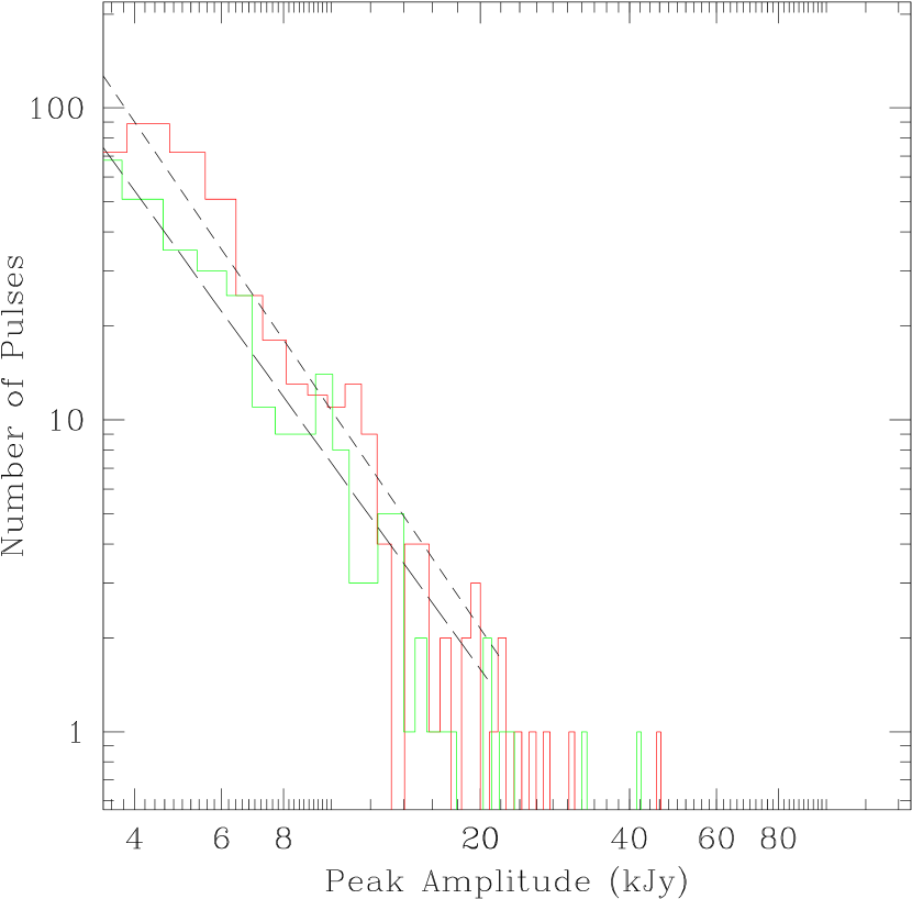
Figure 2: Histograms of giant-pulse amplitudes at 1300 and 1470 MHz (in red and green respectively) constructed from our sample of giant pulses. Estimates for the best fit slope ($\beta$) are $-2.33\pm 0.14$ and $-2.20\pm 0.18$ at 1300 and 1470 MHz respectively, and are shown as short-dashed and long-dashed lines. The brightest pulse detected in our data (at 1300 MHz) has a peak amplitude of $\sim$45 kJy.

3.1 Pulse Amplitudes and Energies

An important distinguishing characteristic of giant pulses (GPs) is their power-law distribution of amplitudes and energies. The amplitude determination can be potentially influenced by factors such as smearing due to instrument and any residual dispersion, as well as external effects such as scattering and scintillation due to the ISM. As a result, oftentimes measurements tend to underestimate the true amplitudes. Observations of Lundgren et al. (1995) and Cordes et al. (2004) (at 430 MHz) were marked by significant instrumental and dispersion smearing (315 and 152 $\mu$s respectively) and were more prone to scintillation and scattering given their observing frequencies $\scriptscriptstyle\stackrel{{\scriptstyle<}}{{\sim}}$ 1 GHz. On the other hand, smearing due to instrument or residual dispersion is negligibly small for baseband observations, and consequently our data enable a better and more accurate characterisation of the pulse amplitudes. Fig. 2 shows the distributions of pulse amplitudes for our data.

The cumulative energy distribution provides a meaningful way of characterizing the frequency of occurrence of GPs. Following Knight et al. (2006), we define this distribution in terms of the probability of a pulse having energy greater than ${E_{0}}$ , and can be expressed as

$$P(E>\mbox{${E_{0}}$\,})=K\,E_{0}^{\alpha}$$ (1)

Figure 3 shows such a distribution for our data. The pulse energy is estimated by integrating the amplitude bins over the extent of emission. The uncertainties in the energy estimates depend on the pulse strength and width, and may range from $\sim$0.5% for strong and narrow pulses, to as much as $\sim$35% for weak, broad pulses. Such large uncertainties at low energies, and possible modulations in pulse amplitudes due to scintillation, may probably explain a gradual flattening seen at low energies. In any case, much in agreement with the earlier work, no evidence is seen for a high-energy cut-off, suggesting that exceedingly bright and energetic pulses are potentially observable over longer durations of observation.

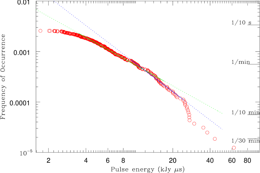
Figure 3: Cumulative distribution of giant-pulse energies at 1300 MHz. The slope estimates of the linear segments below and above an apparent break near $\sim$10 kJy $\mu$s are –1.4 and –1.9 respectively, while the overall slope is –1.6.

Excluding the segments near the low and high ends of the distribution where the behaviour tends to depart from a power-law, we obtain a best-fit value of $-1.59\,\pm\,0.01$ for $\alpha$ (where the error is purely formal) and $K$ = 3.97. Interestingly, this slope is comparable to the published values for other GP-emitters such as PSRs J0218+4232 (Knight et al., 2006), B0540–69 (Johnston et al., 2004) and B1937+21 (Cognard et al., 1996; Soglasnov et al., 2004).

However, it is known from the work of Moffett (1997) that a single slope does not accurately describe the energy distribution at 1400 MHz and that there occurs a break around an energy of $\sim$2 kJy $\mu$s, where the slope $\alpha$ changes from $-3$ to $-1.8$. Given that this energy corresponds to the detection threshold of our GP search (see § 2.5), our slope estimate of $-1.6$ is in general agreement with Moffett’s work. Recent work of Popov & Stappers (2007) suggests that the slope estimate depends on the pulse width, evolving from $-1.7$ to $-3.2$ when going from their shortest (4 $\mu$s) to longest (65 $\mu$s) GPs. Their analysis also shows a clear evidence for a break where the power-law tends to steepen (their Fig. 2). Such a break is also apparent in our data, as the slope tends to steepen near $\sim$10 kJy $\mu$s. Adopting this as the break point, we obtain slope estimates of $-1.37\,\pm\,0.01$ and $-1.88\,\pm\,0.02$ for the segments below and above it (K = 3.72 and 4.42 respectively).

The pulse energy distribution also serves as a useful guide for estimating the rates of occurrence of giant pulses. For instance, on the basis of our observations, a pulse that is about 50 times more energetic than regular pulses can be expected roughly once in 8500 pulse periods, i.e., approximately once every 5 minutes. The most energetic pulse detected in our data has an estimated energy of 66 kJy $\mu$s; i.e. an energy per $\mu$s that is almost $\sim 10^{5}$ times larger than that of regular pulses.

The brightest pulse detected in our data has an estimated peak flux density (${\rm S_{\nu}}$ ) of $\sim$ 45 kJy and an effective width of 0.5 $\mu$s. The equivalent brightness temperature (${\rm T_{b}}$ ) is given by (based on the light-travel size and ignoring relativistic dilation),

$$\mbox{${\rm T_{b}}$\,}=\left({\mbox{${\rm S_{\nu}}$\,}\over 2\,\mbox{${\rm k_{B}}$\,}}\right)\left({D\over\nu\,\mbox{${\delta t}$\,}}\right)^{2},$$ (2)

where $\nu$ is the frequency of observation, ${\delta t}$  is the pulse width, ${\rm k_{B}}$  is the Boltzmann constant and D is the Earth-pulsar distance. The inferred brightness temperature for our strongest pulse is therefore $\sim 10^{35}$ K. This is almost $\sim$1000 times brighter than the brightest pulse detected in the Arecibo observations of Cordes et al. (2004). To the best of our knowledge, this marks the brightest pulse ever recorded from the Crab pulsar within the L-band frequency range (i.e. $\sim$1–2 GHz). Detection of such excessively bright giant pulses offers a promising technique for finding pulsars in external galaxies (Johnston & Romani, 2003; Cordes et al., 2004).

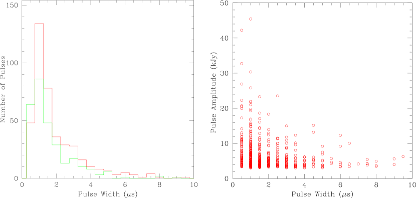
Figure 4: Left: Distributions of giant-pulse widths at 1300 and 1470 MHz (in red and green respectively). Right: Plot of pulse amplitudes vs the effective pulse widths. An apparent low cut-off at 0.5 $\mu$s and a discretization in pulse width are due to the 0.5 $\mu$s final time resolution adopted for our processing.

3.2 Pulse Widths

There have been very few attempts of characterising giant-pulse widths. The first analysis by Lundgren et al. (1995) was limited by their coarse time sampling (205 $\mu$s) and was further constrained by a severe dispersion smearing (70 $\mu$s). More recent work of Popov & Stappers (2007) had a much higher time resolution (4.1 $\mu$s). As our observations were made at a higher frequency than the above (hence the effect of scattering is reduced) and a final time resolution (0.5 $\mu$s) that is eight-fold better than Popov & Stappers (2007), our analysis allows a more accurate characterization of giant-pulse widths.

Our observations show that many giant pulses tend to have a significant structure at 0.5 $\mu$s resolution, ranging from a simple narrow spike to several closely spaced components within a few $\mu$s. Following Lundgren et al. (1995) and Popov & Stappers (2007), we adopt the notion of “effective pulse width” ${W_{e}}$ , which is essentially the averaging time that yields the maximum S/N. In most cases, it is a close representation of true pulse width, although it may be slightly biased to stronger component(s) in the case of highly structured pulses. The histogram of widths obtained in this manner is shown in Fig. 4. The distribution is highly skewed, with measured widths ranging from 0.5 to 10 $\mu$s and with a clear peak at 1 $\mu$s. Giant pulses of widths larger than 10 $\mu$s are absent in our data; however, this may be a selection effect as such pulses may very well be below our detection threshold. Our analysis confirms a general tendency for stronger pulses to be narrower, an observation also noted by Popov & Stappers (2007).

Our distribution of giant-pulse widths can be compared with a similar plot obtained for GPs from the millisecond pulsar PSR B1937+21 by Soglasnov et al. (2004). Similarities in the two distributions are quite striking, despite the fact that GPs from PSR B1937+21 are intrinsically narrower (${W_{e}}$ $\scriptscriptstyle\stackrel{{\scriptstyle<}}{{\sim}}$ 15 ns) and show little structure. Thus, it appears that exponential-tailed distributions are probably common characteristics of giant-pulse widths. Studies of more pulsars are necessary to confirm such a conjecture.

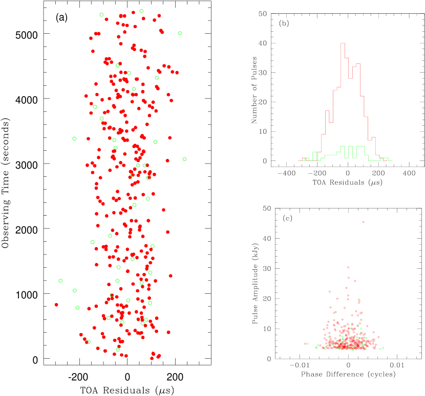
Figure 5: Arrival times of giant pulses detected in the main pulse and interpulse regions (the red and green symbols respectively) at 1300 MHz (left), along with their statistics (right, top) and joint statistics with pulse amplitudes (right, bottom).

3.3 Arrival Times and Phases

One of the most striking properties of Crab GPs is their occurrence within well-defined, relatively narrow longitude ranges of regular radio emission. This is also true with the millisecond pulsars PSRs B1937+21 and J0218+4232, except that in the case of the former, GPs tend to occur near the trailing edges of the main pulse and interpulse (Soglasnov et al., 2004), and in the latter case, they occur near the two minima of the integrated pulse profile (Knight et al., 2006). In order to determine the pulse arrival times, we use the pulsar’s spin-down model along with the TEMPO software package to obtain the anticipated pulse arrival phases. As most pulses in our data are very narrow, our data allow precise determinations of the arrival times and phases. Pulse times-of-arrival (TOAs) obtained in this manner are plotted in Fig. 5.

The total range of longitudes where GPs occur (in the main pulse region) is approximately $\pm$ 200 $\mu$s, or $\pm 2^{\circ}.2$ in angular units, with an RMS of 84 $\mu$s ($0^{\circ}.9$). Thus, a vast majority of GPs (75%) occur within a narrower window of $\pm 100$ $\mu$s. As contributions from the dispersive and instrumental smearing are negligible in our case, this RMS corresponds essentially to the intrinsic pulse-phase jitter and can be compared to a value of 90 $\mu$s estimated by Lundgren et al. (1995) for their data at 800 MHz. The plot of joint statistics of timing residuals and pulse amplitudes shows no obvious correlation except for a general tendency for stronger pulses to originate within narrower phase windows. A similar property was also noted by Cordes et al. (2004) in their Arecibo observations at a frequency of 430 MHz. Finally, a vast majority of GPs tend to occur within the main pulse window $-$ 87% at the main pulse region and the remainder 13% in the interpulse region. This is in excellent agreement with the published values in the literature (Popov & Stappers (2007): 84% and 16% respectively at 1200 MHz; Kostyuk et al. (2003): 86% and 14% respectively at 2228 MHz).

4 Pulse Broadening and Scattering due to the Nebular Plasma

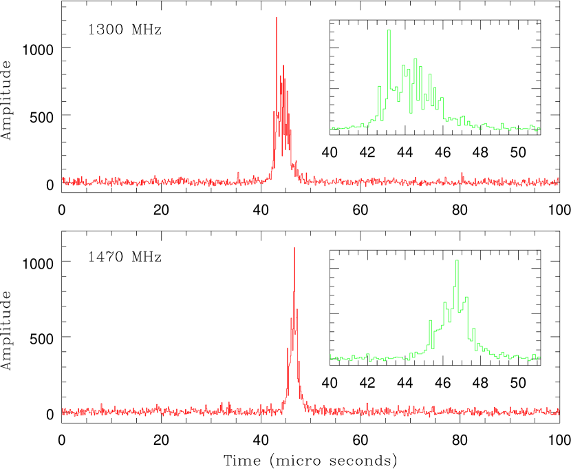
Figure 6: A bright giant pulse at 1300 and 1470 MHz, where the plotted time window corresponds to $\approx$0.003 cycles of the pulsar’s rotation period. This pulse pair is displayed at a time resolution of 128 ns and illustrates significant differences seen in pulse width and structural details between the two frequencies.

4.1 Pulse Shape and Estimation of Scattering

Figure 6 shows an example of a bright giant pulse from our data. At a time resolution of 128 ns, the pulse is resolved into multiple narrow components, and this readily confirms the basic picture of GPs comprising fine structure on very short timescales. Discerning such fine structure is however limited by time resolution and the smearing due to multipath scattering. This pulse pair also exemplifies the differences seen in pulse structure between 1300 and 1470 MHz, a detailed analysis of which is beyond the scope of the present work. Our pulse shapes can be compared to observations of Sallmen et al. (1999) $\sim$10 yr ago (their Fig. 1), and it is striking that our observations are marked by a much lower degree of scattering.

In order to estimate the pulse broadening due to interstellar scattering (e.g. Williamson, 1972; Cordes & Lazio, 2001), we adopt the CLEAN-based deconvolution approach developed by Bhat et al. (2003). Unlike the traditional frequency-extrapolation approach (e.g. Löhmer et al., 2001; Kuzmin et al., 2002), this method makes no prior assumption of the intrinsic pulse shape, and thus offers a more robust means of determining the underlying pulse broadening function (PBF). The procedure involves deconvolving the measured pulse shape in a manner quite similar to the CLEAN algorithm used in synthesis imaging, while searching for the best-fit PBF and recovering the intrinsic pulse shape. It relies on a set of figures of merit that are defined in terms of positivity and symmetry of the resultant deconvolved pulse and some parameters characterizing the noise statistics in order to determine the best-fit PBF. For the purpose of our analysis, we assume the simplest and most commonly used form for the PBF that corresponds to a thin-slab scattering screen geometry. The functional form for such a PBF is a one-sided exponential (e.g. Williamson, 1972) and is given by

$$G(t)=\left({1\over\tau_{d}}\right)\,\exp\left({-t\over\mbox{${\rm\tau_{d}}$\,}}\right)\,U(t),$$ (3)

where $U(t)$ is the unit step function, $U(<0)=0,U(\geq 0)=1$. Fig. 7 shows the best-fit PBF and the reconstructed pulse obtained in this manner. The ${\rm e^{-1}}$ point of this PBF is the scattering time ${\rm\tau_{d}}$ , for which our deconvolution procedure yields an estimate of $0.8\pm 0.4$ $\mu$s.

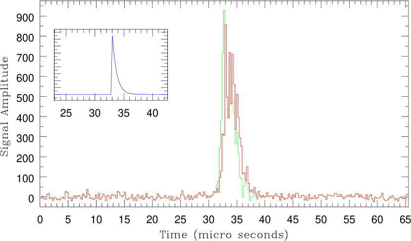
Figure 7: A bright giant pulse from observations at 1300 MHz. The time window corresponds to 0.002 cycles of the pulse period. The reconstructed pulse (green) and the best-fit pulse-broadening function (inset) from our deconvolution procedure are also shown. The $e^{-1}$ point of this one-sided exponential gives an estimate of the pulse-broadening time, for which our measured value is $0.8\pm 0.4$ $\mu$s.

This measurement of a low scattering is further supported by the following observational facts. First, a pulse broadening of $\sim$0.8 $\mu$s will imply rapid intensity decorrelations in frequency on characteristic scales $\sim 1/2\pi\mbox{${\rm\tau_{d}}$\,}$ $\sim$ 0.1 to 0.3 MHz and this is confirmed by our analysis. Second, as seen in Fig. 4, a large number of pulses detected in our data have widths $\sim$1 $\mu$s, just about what we would expect given the $\sim$0.8 $\mu$s broadening due to scattering and the 0.5 $\mu$s time resolution.

4.2 Scattering due to the Nebula

Our measurement of ${\rm\tau_{d}}$ can be compared to that reported by Sallmen et al. (1999) based on their observations in 1996. Their value of $95\pm 5$ $\mu$s at 600 MHz would scale to 4.3 $\mu$s at 1300 MHz, assuming a canonical $\nu^{-4}$ dependence expected from scattering due to a turbulent plasma screen. This is five times larger than our measurement. A somewhat smaller value is expected on the basis of observations of Kuzmin et al. (2002) in the year 2000. However, our measurement is consistent with that of Bhat et al. (2007) at 200 MHz, if we extrapolate their measurements using their revised frequency scaling of $\nu^{-3.5\pm 0.2}$.

As described in § 2.3, our GP detection procedure includes determination of the best DM by performing dedispersion over many trial values around its nominal value. As most pulses in our data are very narrow, this procedure allows a precise determination of the Crab’s true DM at our observing epoch. An estimate of $56.751\pm 0.001$ ${\rm pc\ cm^{-3}}$ obtained in this manner is further confirmed by measuring the time delay between the pulse arrival times at 1300 and 1470 MHz. This value is in excellent agreement with that reported in the Jodrell Bank (JB) monthly ephemeris (Lyne, 1982) on the nearest date of our observing, but it is significantly lower than that measured near the observing epochs of Sallmen et al. (1999).

Thus, over a 10-yr time span between Sallmen et al’s and our observations, the pulsar’s DM decreased by 0.09 ${\rm pc\ cm^{-3}}$ while the pulse broadening decreased by a factor of 5. Given the strong frequency dependence of pulse broadening ($\mbox{${\rm\tau_{d}}$\,}\propto\nu^{-x}$) and the observational evidence for the scaling index $x$ changing over the time (Kuzmin et al., 2002; Bhat et al., 2007), it is more meaningful to adopt a frequency independent parameter such as the scattering measure (SM) for comparison purposes. This parameter quantifies the total scattering along the line of sight (LOS) and is defined as the LOS integral of ${C_{n}^{2}}$ , which is the spectral coefficient of the wavenumber spectrum of electron density irregularities. It can be related to ${\rm\tau_{d}}$ via the relation $\mbox{${\rm\tau_{d}}$\,}\approx 1.1\,\mbox{$W_{\tau}$}~{}{\rm SM}^{6/5}\nu^{-x}D$, where $\nu$ is in GHz, D is in kpc, and $W_{\tau}$ is a geometric factor that depends on the LOS-distribution of scattering material (Cordes & Rickett, 1998). Assuming $\mbox{$W_{\tau}$}=1$, we can estimate the effective SM for a uniform medium, and for the measurements of Sallmen et al’s and ours, we obtain values of $1.3\times 10^{-2}$ and $3\times 10^{-3}$ ${\rm kpc\ m^{-20/3}}$ respectively. That is, the SM changed by 0.01 ${\rm kpc\ m^{-20/3}}$ when the DM changed by 0.09 ${\rm pc\ cm^{-3}}$ , or a factor 4 decrease in the scattering strength associated with a DM change of only 0.16%.

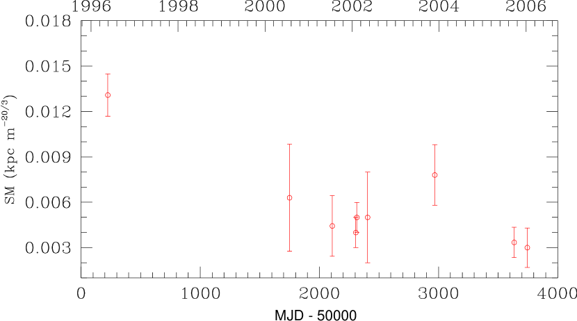
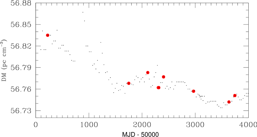
Figure 8: Measurements of DM and SM of the Crab pulsar from observations over the past 10 years (1996 to 2006). The SM values (upper panel) are estimated from the published pulse-broadening measurements and decorrelation bandwidths – 1996.4: Sallmen et al. (1999); 2000.6: Kostyuk et al. (2003); 2001.5: Kuzmin et al. (2002); 2002.1, 2002.4: Cordes et al. (2004); 2003.9: Popov et al. (2006); 2005.6: Bhat et al. (2007); 2006.0: our observations. The DM measurements are from the Jodrell Bank monthly ephemeris (lower panel); the thick solid circles correspond to the observing epochs of the SM measurements.

A closer look at the JB ephemeris reveals quite a systematic decrease in the Crab’s DM variations between 1996 and 2006, with the lowest DM recorded near mid-2005 and a reversal of the trend in early 2006. A plot of SM estimates for the available ${\rm\tau_{d}}$ measurements during this period is shown in Fig. 8 along with the DM measurements at relevant epochs. These plots illustrate a gradual reduction in the Crab’s DM and scattering over this 10-yr time span. Such variations are too large and smooth to be caused by refractive scintillation effects in the ISM, and are therefore indicative of a nebular origin.

The material within the Crab Nebula, specifically the perturbed thermal plasma associated with it, has often been advanced as the source of excessive scattering and anomalous DM variations on several occasions. The most remarkable observations in support of this are the anomalous scattering recorded in 1974-1975 (Lyne & Thorne, 1975; Isaacman & Rankin, 1977) and the reflection event in 1997 (Backer et al., 2000; Lyne et al., 2001). The scattering event in 1974 was especially noted for its extreme activity, where the pulsar’s DM rose by 0.07 ${\rm pc\ cm^{-3}}$ and the scattering increased by an order an magnitude over a time span of several months. Isaacman & Rankin (1977) ascribed this to a two-component scattering-screen model where the variable screen associated with the nebula gives rise to such rapid changes in both DM and scattering. The anomalous dispersion event in 1997 was seen as discrete moving echoes of the pulse, and was interpreted as reflections from an ionized shell in the outer parts of the nebula by Lyne et al. (2001), and in terms of variable optics of a triangular prism located in the interface of the nebula and the supernova ejecta by Backer et al. (2000).

Fig. 8 reveals a similar change in DM and a large but less dramatic change in scattering. A direct interpretation of such observations can be made along the lines of a variable scattering screen model, as we discuss in detail in the following section.

4.3 Implications for the Nebular Structure and Densities

The observed changes in DM and SM can be used to constrain the combination of the electron density and the “fluctuation parameter” in the nebular region, denoted as ${n_{e,cn}}$ and ${F_{cn}}$ respectively. Following Cordes & Lazio (2003) and Bhat et al. (2004), the measured decrements in DM and SM can be expressed as $\mbox{${\delta DM}$\,}=\mbox{${n_{e,cn}}$\,}\mbox{${\delta s}$\,}$ and $\mbox{${\delta SM}$\,}=\mbox{${C_{n,cn}^{2}}$\,}\mbox{${\delta s}$\,}$, where ${\delta s}$ is the size of the nebular scattering region and ${C_{n,cn}^{2}}$ is the equivalent turbulent intensity (assuming a uniform distribution of scattering material). The parameters ${F_{cn}}$ and ${C_{n,cn}^{2}}$ can be related as (Taylor & Cordes, 1993; Cordes & Lazio, 2002) $\mbox{${C_{n,cn}^{2}}$\,}=\mbox{${C_{SM}}$\,}\mbox{${F_{cn}}$\,}\mbox{${n_{e,cn}^{2}}$\,}$, where $\mbox{${C_{SM}}$\,}=[3(2\pi)^{1/3}]^{-1}\,\mbox{${K_{u}}$\,}$ for a Kolmogorov spectrum, and ${K_{u}}$  =10.2 ${\rm m^{-20/3}cm^{6}}$  to yield SM in units of ${\rm kpc\ m^{-20/3}}$ . The above expressions can be combined to yield the ratio of ${\delta SM}$ and ${\delta DM}$ , and is given by

$${\mbox{${\delta SM}$\,}\over\mbox{${\delta DM}$\,}}=\mbox{${C_{SM}}$\,}\mbox{${F_{cn}}$\,}\mbox{${n_{e,cn}}$\,}$$ (4)

Thus our measurements of ${\delta SM}$ = 0.01 ${\rm kpc\ m^{-20/3}}$  and ${\delta DM}$ = 0.09 ${\rm pc\ cm^{-3}}$ yield ${F_{cn}}$ ${n_{e,cn}}$ = 55. The fluctuation parameter is essentially a product of normalized variances (at small and large scales) and other terms such as the outer scale and filling factor. The electron density ${n_{e,cn}}$ is unknown, but assuming a nominal value of 1 ${\rm cm^{-3}}$ , we get ${F_{cn}}$ = 55, which is much larger than that typical of the Galactic spiral arms ($F\sim 10$).

The large values of ${\delta SM}$ and ${F_{cn}}$ indeed confirm the material within the nebula as the source of excessively strong scattering. While the scattering and dispersion events of 1974 and 1997 were interpreted in terms of a single large structure with electron density $\sim$1,500 ${\rm cm^{-3}}$ , the long-term systematic variations in dispersion and scattering as shown in Fig. 8 can be interpreted in terms of a scenario whereby the nebular segment of the LOS is populated by many smaller structures of much lower densities. A variation in the number density of such structures may then account for the observed changes in DM and SM. As the nebula is thought to comprise fine structure on many length scales, perhaps even on scales much finer than the filamentary structure suggested by optical observations (e.g. Hester et al., 1995), such a picture seems quite plausible.

For the sake of simplicity, if we model the measured changes in scattering and dispersion to arise from N such structures of size ${\delta s_{sc}}$ and density ${n_{e,sc}}$ , the resultant contributions to SM and DM are given by

$$\mbox{${\delta SM}$\,}\equiv\sum_{i=1}^{i=N}\mbox{${SM_{sc,i}}$\,}=N\,\mbox{${C_{SM}}$\,}\mbox{${F_{sc}}$\,}\mbox{${n_{e,sc}^{2}}$\,}\mbox{${\delta s_{sc}}$\,}$$ (5)

$$\mbox{${\delta DM}$\,}\equiv\sum_{i=1}^{i=N}\mbox{${DM_{sc,i}}$\,}=N\,\mbox{${n_{e,sc}}$\,}\mbox{${\delta s_{sc}}$\,}$$ (6)

Following equations (4)–(6) and the constraint $\mbox{${F_{cn}}$\,}\mbox{${n_{e,cn}}$\,}=55$, the electron density of such a structure can be estimated as

$$\mbox{${n_{e,sc}}$\,}=\left({\mbox{${\delta SM}$\,}\over 55\,\mbox{${C_{SM}}$\,}}\right)\left({1\over N\,\mbox{${\delta s_{sc}}$\,}}\right)$$ (7)

Thus, with just two direct measurements alone (${\delta DM}$ and ${\delta SM}$ ), it is hard to constrain all 3 free parameters of the model. However, assuming a reasonable value for ${\delta s_{sc}}$ $\sim$ $10^{-5}$ pc (i.e. an order of magnitude smaller than that implied by the 1997 reflection event), we estimate ${n_{e,sc}}$ $\sim$ 100 ${\rm cm^{-3}}$ for N$\sim$100. This is almost an order of magnitude smaller than the densities required to produce the reflection event. Indeed, several different combinations of size and density are possible; nonetheless, the underlying picture is the presence of many moderately-dense structures in the nebular region, with a filling factor $\sim$ $10^{-3}$.

We note that the electron density estimated above, estimates of the electron temperature in the Crab nebula (Temim et al., 2006; Hester et al., 1995; Davidson, 1979) that yield values between 6000 and 16000 K, and the size of the Crab nebula (approximately $6^{\prime}$ = 3 pc, for a distance of 2 kpc), imply that the nebula should produce a minimal optical depth to free-free absorption at GHz frequencies and a significant optical depth at lower frequencies. We estimate, based on these parameters, that a free-free optical depth ($\tau_{ff}$) of 0.007 at 1 GHz may be possible, along lines of sight that include the scattering structures discussed above. For radio sources behind the Crab nebula, this would give a decrease in the observed flux density, compared to the intrinsic flux density, of 0.7% due to free-free absorption at this frequency. At lower frequencies this decrease would be more significant: 3% at 500 MHz, 12% at 250 MHz, and 60% at 100 MHz.

If a radio interferometer operating at these frequencies could achieve an angular resolution high enough to resolve the Crab nebula and detect compact sources of emission behind the nebula, it may be possible to survey the free-free absorption due to the nebula along many lines of sight, probing the structures that are producing the scattering of the pulsar emission. The upcoming future instruments such as the extended LOFAR telescope in The Netherlands and Europe, or the Murchison Wide-field Array (MWA) in Western Australia may be able to undertake such a survey.

5 Summary and Conclusions

Using the ATCA and a baseband recording system, we detected more than 700 giant pulses from the Crab pulsar from our continuous and uniform recording at 1300 and 1470 MHz over 3 hours. This large sample is used for investigating statistical properties of giant pulses, such as their amplitude, width, arrival time and energy distributions. The amplitude distribution follows roughly a power-law with a slope of $-2.33\pm 0.15$, which is shallower compared to those from previous observations at lower frequencies. The pulse widths show an exponential-tailed distribution and there is a tendency for stronger pulses to be narrower. A majority of pulses (87%) tend to occur within a narrow phase window ($\pm 200$ $\mu$s) of the main-pulse region. Finally, the distribution of pulse energies follows a power-law with a slope of $-1.6$, and there is evidence for a break near $\sim$10 kJy $\mu$s.

The brightest pulse detected in our data has a peak amplitude of 45 kJy and a width of 0.5 $\mu$s, implying a brightness temperature of $10^{35}$ K, which makes it the brightest pulse recorded from the Crab pulsar at the L-band frequencies (1–2 GHz).

Our observations show that many giant pulses comprise multiple narrow components at a time resolution $\sim$128 ns, which confirms the fundamental picture of giant pulses being superpositions of extremely narrow bursts. Further, the measured pulse shape is marked by an unusually low degree of scattering, with a pulse-broadening time of $0.8\pm 0.4$ $\mu$s that is the lowest estimated yet towards the Crab from observations so far. Further, the pulsar’s DM is determined to be $56.751\pm 0.001$ ${\rm pc\ cm^{-3}}$ , which is significantly lower than those measured near the epochs of previous scattering measurements.

Our measurements of DM and scattering, together with published data and the Jodrell Bank monthly ephemeris, unveil a systematic and slow decrease in the Crab’s DM and scattering over the past 10 yr. These variations are too large and smooth to be caused by the intervening ISM but can be attributed to the material within the nebula. Our analysis hints at there being large-scale inhomogeneities in the distribution of small-scale density structures in the nebular region, with a plausible interpretation involving many ($\sim$ 100) dense ($\sim$100 ${\rm cm^{-3}}$ ) structures. A variation in their number density or size can potentially lead to the observed changes in DM and scattering. Such a possibility can be further investigated by obtaining independent constraints on the nebular electron densities (e.g. via free-free absorptions at low radio frequencies) and through future observations to monitor the pulsar’s DM and scattering.

Acknowledgements: The ATCA is part of the Australia Telescope, which is funded by CSIRO for operation as a National Facility by ATNF. Data processing was carried out at Swinburne University’s Supercomputing Facility. We thank Matthew Bailes and Simon Johnston for fruitful discussions, and Willem van Straten and Joris Verbiest for a critical reading of the manuscript. We also thank the referee for a critical review and several inspiring comments and suggestions that helped improve the presentation and clarity of the paper. This work is supported by the MNRF research grant to Swinburne University of Technology.

References

- Argyle & Gower (1972) Argyle, E., & Gower, J. F. R. 1972, ApJ, 175, L89
- Backer et al. (2000) Backer, D. C., Wong, T., & Valanju, J. 2000, ApJ, 543, 740
- Bietenholz et al. (1997) Bietenholz, M. F., Kassim, N., Frail, D. A., Perley, R. A., Erickson, W. C., & Hajian, A. R. 1997, ApJ, 490, 2991
- Bhat et al. (2003) Bhat, N. D. R., Cordes, J. M. & Chatterjee, S. 2003, ApJ, 584, 782
- Bhat et al. (2004) Bhat, N. D. R., Cordes, J. M., Camilo, F., Nice, D. J., & Lorimer, D. R. 2004, ApJ, 605, 759
- Bhat et al. (2007) Bhat, N. D. R., et al. 2007, ApJ, 665, 618
- Cognard et al. (1996) Cognard, I., Shrauner, J. A., Taylor, J. H., & Thorsett, S. E. 1996, ApJ, 457, L81
- Cordes et al. (2004) Cordes, J. M., Bhat, N. D. R., Hankins, T. H., McLaughlin, M. A., & Kern, J. 2004, ApJ, 612, 375
- Cordes & Lazio (2001) Cordes, J. M., & Lazio, T. J. W. 2001, ApJ, 549, 997
- Cordes & Lazio (2002) Cordes, J. M., & Lazio, T. J. W. 2002, arXiv:astro-ph/0207156
- Cordes & Lazio (2003) Cordes, J. M., & Lazio, T. J. W. 2003, arXiv:astro-ph/0301598
- Cordes & Rickett (1998) Cordes, J. M., & Rickett, B. J. 1998, ApJ, 507, 846
- Davidson (1979) Davidson, K. 1979, ApJ, 228, 179
- Hankins (1971) Hankins, T. H. 1971, ApJ, 169, 487
- Hankins & Rickett (1975) Hankins, T. H., & Rickett, B. J. 1975, Methods in Computational Physics. Volume 14 - Radio astronomy, 14, 55
- Hankins et al. (2003) Hankins, T. H., Kern, J. S., Weatherall, J. C., & Eilek, J. A. 2003, Nature, 422, 141
- Hesse & Wielebinski (1974) Hesse, K. H., & Wielebinski, R. 1974, A&A, 31, 409
- Hester et al. (1995) Hester, J. J., et al. 1995, ApJ, 448, 240
- Isaacman & Rankin (1977) Isaacman, R., & Rankin, J. M. 1977, ApJ, 214, 214
- Johnston & Romani (2003) Johnston, S., & Romani, R. W. 2003, ApJ, 590, L95
- Johnston et al. (2004) Johnston, S., Romani, R. W., Marshall, F. E., & Zhang, W. 2004, MNRAS, 355, 31
- Hester et al. (1995) Hester, J. J., et al. 1995, ApJ, 448, 240
- Knight et al. (2006) Knight, H. S., Bailes, M., Manchester, R. N., Ord, S. M., & Jacoby, B. A. 2006, ApJ, 640, 941
- Kostyuk et al. (2003) Kostyuk, S. V., Kondratiev, V. I., Kuzmin, A. D., Popov, M. V., & Soglasnov, V. A. 2003, Astronomy Letters, 29, 387
- Kuzmin et al. (2002) Kuzmin, A. D., Kondrat’ev, V. I., Kostyuk, S. V., Losovsky, B. Y., Popov, M. V., Soglasnov, V. A., D’Amico, N., & Montebugnoli, S. 2002, Astronomy Letters, 28, 251
- Löhmer et al. (2001) Löhmer, O., Kramer, M., Mitra, D., Lorimer, D. R., & Lyne, A. G. 2001, ApJ, 562, L157
- Lundgren et al. (1995) Lundgren, S. C., Cordes, J. M., Ulmer, M., Matz, S. M., Lomatch, S., Foster, R. S., & Hankins, T. 1995, ApJ, 453, 433
- Lyne & Thorne (1975) Lyne, A. G., & Thorne, D. J. 1975, MNRAS, 172, 97
- Lyne (1982) Lyne, A. G., Jodrell Bank Crab Pulsar Monthly Ephemeris (http://www.jb.man.ac.uk/pulsar/crab.html)
- Lyne et al. (2001) Lyne, A. G., Pritchard, R. S., & Graham-Smith, F. 2001, MNRAS, 321, 67
- Manchester et al. (2005) Manchester, R. N., Hobbs, G. B., Teoh, A., & Hobbs, M. 2005, AJ, 129, 1993
- Moffett (1997) Moffett, D. A. 1997, Ph.D. Thesis
- Moffett & Hankins (1996) Moffett, D. A., & Hankins, T. H. 1996, ApJ, 468, 779
- Popov et al. (2006) Popov, M. V., et al. 2006, Astronomy Reports, 50, 562
- Popov & Stappers (2007) Popov, M. V., & Stappers, B. 2007, A&A, 470, 1003
- Rankin & Counselman (1973) Rankin, J. M., & Counselman, C. C., III 1973, ApJ, 181, 875
- Sallmen et al. (1999) Sallmen, S., Backer, D. C., Hankins, T. H. et al. 1999, ApJ, 517, 460
- Soglasnov et al. (2004) Soglasnov, V. A., Popov, M. V., Bartel, N. et al. 2004, ApJ, 616, 439
- Staelin & Reifenstein (1968) Staelin, D. H., & Reifenstein, E. C. 1968, Science, 162, 1481
- Taylor & Cordes (1993) Taylor, J. H., & Cordes, J. M. 1993, ApJ, 411, 674
- Temim et al. (2006) Temim, T., et al. 2006, AJ, 132, 1610
- van Straten (2003) van Straten, W. 2003, PhD thesis, Swinburne Univ. of Technology
- Williamson (1972) Williamson, I. P. 1972, MNRAS, 157, 55