SNUTP 07-013

Minimal gauge inflation

Jinn-Ouk Gong^1,2   and   Seong Chan Park^3
1 Harish-Chandra Research Institute
Chhatnag Road, Jhunsi, Allahabad 211 019, India
² Department of Physics, University of Wisconsin-Madison
1150 University Avenue, Madison, WI 53706-1390, USA
³ Frontier Physics Research Division
School of Physics and Astronomy, Seoul National University
Seoul 151-747, Republic of Korea

We consider a gauge inflation model in the simplest orbifold $M_{4}\times S^{1}/\mathbb{Z}_{2}$ with the minimal non-Abelian $SU(2)$ hidden sector gauge symmetry. The inflaton potential is fully radiatively generated solely by gauge self-interactions. Following the virtue of gauge inflation idea, the inflaton, a part of the five dimensional gauge boson, is automatically protected by the gauge symmetry and its potential is stable against quantum corrections. We show that the model perfectly fits the recent cosmological observations, including the recent WMAP 5-year data, in a wide range of the model parameters. In the perturbative regime of gauge interactions ($g_{\rm 4D}\lesssim 1/(2\pi RM_{\rm Pl})$) with the moderately compactified radius ($10\lesssim RM_{\rm Pl}\lesssim 100$) the anticipated magnitude of the curvature perturbation power spectrum and the value of the corresponding spectral index are in perfect agreement with the recent observations. The model also predicts a large fraction of the gravitational waves, negligible non-Gaussianity, and high enough reheating temperature.

1 Introduction

It is now widely accepted that an early period of accelerated expansion of the universe, or inflation [1], can resolve many cosmological problems such as horizon problem and can provide the desired initial conditions for the subsequent hot big bang evolution of the observed universe [2]. Many observational facts such as the flatness of the universe and the isotropy of the cosmic microwave background (CMB) are natural consequences of inflation, and hence they strongly support the existence of such a period of acceleration in the very early universe. In particle physics point of view, inflation occurs when one or more scalar fields, the inflaton fields, dominate the energy density of the universe with their potential being overwhelming [3]. Under such a condition, dubbed slow-roll condition, curvature perturbation $\mathcal{R}$ is produced which is nearly scale invariant and is heavily constrained by the measurements of the anisotropies of the CMB and the observations of the large scale structure [4], including the recent Wilkinson Microwave Anisotropy Probe (WMAP) 5-year data set [5]. The slow-roll condition says that the inflaton potential should be very flat, i.e. the effective mass of the inflaton should be very small compared with the inflationary Hubble parameter. This is, however, quite difficult to be achieved: for example, in supergravity, any generic scalar field is expected to have an effective mass of $\mathcal{O}(H)$ [6], which completely spoils the desired slow-roll condition. It is thus natural to consider some symmetry principle which protects the small inflaton mass from large radiative corrections or supergravity effects.

Shift symmetry, under which the field is invariant with respect to the transformation

$$\phi\to\phi+a\,,$$ (1)

with $a$ being an arbitrary constant, is one of such symmetries and the corresponding fields remain completely massless, i.e. their potential is exactly flat as long as shift symmetry is unbroken. When the symmetry is explicitly broken, they become pseudo Nambu-Goldstone bosons (pNGBs) and the potential acquires a tilt depending on the symmetry breaking scale $f$ and is of the form

$$V(\phi)=\Lambda^{4}\left[1\pm\cos\left(\frac{\phi}{f}\right)\right]\,.$$ (2)

The model of natural inflation [7] makes use of such a pNGB with large $f$, which renders the potential very flat. This largeness, however, requires $f\gg M_{\rm Pl}\equiv G^{-1/2}\sim 10^{19}\mathrm{GeV}$ and hence the valid region of successful natural inflation lies in the regime where we completely lose theoretical control. This has been regarded as a significant drawback of natural inflation.

An idea to evade this problem was suggested in Ref. [8]. In this scenario, called gauge inflation, the inflaton field is essentially coming from a part of the fifth component of the gauge boson in five dimensional bulk $A_{5}$, by which the gauge invariant Wilson line is defined as

$$e^{i\theta}\equiv\exp\left[ig\oint A_{5}dy\right]\,,$$ (3)

where $g$ is the gauge coupling constant. By the one-loop interactions with the charged particles, the potential of the canonically normalized field $\phi\equiv f\theta$ has basically the same form as Eq. (2) while $f=1/(g_{4}L)$ has extra dimensional nature with $L$ being the size of the fifth dimension. Hence the potential can be trusted even when $f$ is larger than $M_{\rm Pl}$ in the perturbative regime of gauge interaction, $g_{4}\lesssim 1/(M_{\rm Pl}L)$. An interesting possibility to unify the grand unification theory (GUT) and cosmic inflation in the framework of the gauge inflation was suggested in Ref. [10] by one of the authors of the present paper: starting from the higher dimensional $SU(5)$ GUT, the standard model is recovered by orbifold projection by $S^{1}/{\mathbb{Z}_{2}}$ and a massless scalar boson from the fifth component of the gauge boson is shown to play the role of the inflaton with a fully radiatively generated flat potential.

In this paper, we take a different approach. Here we try to build the minimal model of gauge inflation using the simplest orbifold $S^{1}/\mathbb{Z}_{2}$ and the minimal non-Abelian gauge group $SU(2)$ for the hidden sector. The obvious advantages of this approach is two-fold. First, by taking the hidden sector gauge interaction, the theory is less constrained than the visible sector gauge theory, e.g. GUT [10]. This is important since the required coupling constant is typically very small, $g_{4}\sim 10^{-2}$, so it is hard to reconcile this smallness with the coupling constant unification. Second, the minimality can apply to the particle contents. Different from the Abelian case, the non-Abelian gauge theory accommodates the gauge self-interactions by which the potential for the inflaton ($\sim A_{5}$) can be generated even without any additional charged matter fields. So the theory remains minimal in particle contents and its predictions are quite robust and free from parameters such as the masses and other quantum numbers of newly introduced matter fields. Combining the minimal choice of the orbifold and the gauge group, no exotic particles appear in the theory. The model is clean.

The structure of the paper is as follows. In the next section, we give the detail of the higher dimensional gauge theory and outline the subsequent cosmological scenario. Section 3 is devoted to the cosmological evolution of the model and we analytically calculate the observable quantities produced during inflation and study their relations to the parameters of the model. We also address the issue of reheating and estimate the reheating temperature $T_{\mathrm{RH}}$. In Section 4 we then conclude.

2 The model

As we already emphasized in the previous section, we do not wish to introduce any exotic particle in the hidden sector. So non-Abelian gauge symmetry is introduced and the minimal choice is $SU(2)$. The spacetime is five dimensional where the fifth dimension is compactified by an orbifold $S^{1}/\mathbb{Z}_{2}$.

The $SU(2)$ gauge theory on the orbifold is constructed by specifying two independent parity conditions at the two fixed points, $y=0$ and $y=\pi R$ where $R$ is the compactification radius, as

$$A_{\mu}(x,-y)= P_{0}A_{\mu}(x,y)P_{0}\,,$$ (4)

$$A_{5}(x,-y)= -P_{0}A_{5}(x,y)P_{0}\,,$$ (5)

$$A_{\mu}(x,\pi R-y)= P_{1}A_{\mu}(x,\pi R+y)P_{1}\,,$$ (6)

$$A_{5}(x,\pi R-y)= -P_{1}A_{5}(x,\pi R+y)P_{1}\,,$$ (7)

where $P_{0}$ and $P_{1}$ are $2\times 2$ matrices satisfying $P_{0}^{2}=P_{1}^{2}=1$. The translational transformation, $y\rightarrow y+2\pi R$, is generated by successive operation of the parity operators, $P_{1}P_{0}$. Taking $P_{0}=P_{1}=\mathrm{diag}(1,-1)$, at the classical level the gauge symmetry $SU(2)$ is reduced to $U(1)$ by the orbifold projection. Here we explicitly write down the parity assignment with $P_{0}$ and $P_{1}$ as

$$A_{\mu} =\left(\begin{array}[]{cc}(++)&(--)\\ (--)&(++)\\ \end{array}\right),$$ (10)

$$A_{5} =\left(\begin{array}[]{cc}(--)&(++)\\ (++)&(--)\\ \end{array}\right),$$ (13)

thus the zero modes are $A_{\mu}^{3}$ and $A_{5}^{1,2}$ which correspond to the $H=U(1)$ gauge boson, i.e. mirror photon and the scalar field, respectively. The scalar field $A_{5}^{1,2}$ may develop a vacuum expectation value which could be put into the form of $A_{5}^{a}\sim(\phi,0,0)$ due to the remaining $U(1)$ global symmetry. Taking into account the effects from the gauge, ghost and the scalar self interaction, the one-loop effective potential for the field $\phi$ is induced as

$$V_{\rm 1-loop}(\phi)=-\frac{9}{(2\pi)^{6}R^{4}}\sum_{n=1}^{\infty}\frac{\cos(n\phi/f_{\rm eff})}{n^{5}}\,,$$ (14)

where the effective decay constant

$$f_{\rm eff}\equiv\frac{1}{\sqrt{2\pi R}g}=\frac{1}{2\pi g_{\rm 4D}R}$$ (15)

is introduced for canonical normalization of $\phi$ [11] (also see [13]). Here we can add a cosmological constant

$$\frac{9\zeta(5)}{(2\pi)^{6}R^{4}}\,,$$ (16)

where $\zeta(5)=\sum_{n=1}^{\infty}n^{-5}$, so that $V_{\mathrm{1-loop}}(0)=0$ to solve the cosmological constant problem, which we do not attempt to address. Thus, the radiatively generated inflaton potential is the sum of Eqs. (14) and (16), i.e.

$$V(\phi)=\frac{9}{(2\pi)^{6}R^{4}}\sum_{n=1}^{\infty}\frac{1}{n^{5}}\left[1-\cos\left(\frac{n\phi}{f_{\rm eff}}\right)\right]\,.$$ (17)

In principle, we can further introduce additional matter field(s) with charge $q$ in the hidden sector but for the simplicity and predictability we introduce none. In this sense, our model, which may be responsible for the cosmological inflation, is the minimal model of hidden sector gauge theory on the simplest orbifold in five dimensions. After an inflationary epoch achieved while $\phi$ rolls down the effective potential given by Eq. (17), it oscillates at the minimum and decays to reheat the universe. After then the standard hot big bang evolution follows. In the next section we calculate the observable quantities produced during inflation and confirm the relevance of our model.

3 Cosmological evolution

In this section, we study the detail of the cosmological evolution of the model described in the previous section. For analytic simplicity, we take as the leading approximation only the first term of the sum in Eq. (17), i.e.

$$V(\phi)\approx\frac{9}{(2\pi)^{6}R^{4}}\left[1-\cos\left(\frac{\phi}{f_{\rm eff}}\right)\right]\,.$$ (18)

As we will see in Table 1, this approximation works fairly good. Then the potential is identical to that of natural inflation, Eq. (2), and the analytic calculations are straightforward especially when $\phi$ is close to the top [14]. Here we just give the results of the observable quantities: the power spectrum of the curvature perturbation $\mathcal{P}_{\mathcal{R}}$, the corresponding spectral index $n_{\mathcal{R}}$, the tensor-to-scalar ratio $r$ and the non-linear parameter $f_{\mathrm{NL}}$ [15]. Under the slow-roll approximation, they are given by

$$\mathcal{P}_{\mathcal{R}}^{1/2}= \sqrt{\frac{8V}{3\epsilon M_{\rm Pl}^{4}}}\,,$$ (19)

$$n_{\mathcal{R}}= 1-6\epsilon+2\eta\,,$$ (20)

$$r= 16\epsilon\,,$$ (21)

$$-\frac{3}{5}f_{\mathrm{NL}}= \frac{1}{2}\left[\left(3+f_{k}\right)\epsilon-\eta\right]\,,$$ (22)

respectively. Here, $\epsilon$ and $\eta$ are the usual slow-roll parameters and are defined by

$$\epsilon\equiv \frac{M_{\rm Pl}^{2}}{16\pi}\left(\frac{V^{\prime}}{V}\right)^{2}\,,$$ (23)

$$\eta\equiv \frac{M_{\rm Pl}^{2}}{8\pi}\frac{V^{\prime\prime}}{V}\,,$$ (24)

where a prime denotes a derivative with respect to $\phi$, and $f_{k}$ is a constant in the range of $0\leq f_{k}\leq 5/6$, depending on the momenta [16]. Note that the running of $n_{\mathcal{R}}$, which in the slow-roll approximation is written as

$$\frac{dn_{\mathcal{R}}}{d\log{k}}=-16\epsilon\eta+24\epsilon^{2}+2\xi^{2}\,,$$ (25)

with

$$\xi^{2}\equiv\frac{M_{\rm Pl}^{4}}{64\pi^{2}}\frac{V^{\prime}V^{\prime\prime\prime}}{V^{2}}$$ (26)

being another slow-roll parameter, is second order in the slow-roll approximation and is negligibly small compared with the other quantities, so here we do not compute it while the calculation is straightforward. Also, the running of $r$ [18],

$$\frac{d\log{r}}{d\log{k}}=2(2\epsilon-\eta)\,,$$ (27)

is another first order quantity and thus could be observable, but we can obtain the same result by combining Eqs. (20) and (21) although it can serve as a consistency check. Writing Eqs. (19), (20), (21) and (22) in terms of $f_{\rm eff}$ and $R$ as Eq. (17), we can obtain

$$\mathcal{P}_{\mathcal{R}}^{1/2}= \frac{8\sqrt{3}}{(2\pi)^{5/2}}\frac{f_{\rm eff}/M_{\rm Pl}}{(RM_{\rm Pl})^{2}}\left\{2-\frac{32\pi(f_{\rm eff}/M_{\rm Pl})^{2}}{16\pi(f_{\rm eff}/M_{\rm Pl})^{2}+1}\exp\left[\frac{-N}{8\pi(f_{\rm eff}/M_{\rm Pl})^{2}}\right]\right\}$$

$$\times\left\{\frac{32\pi(f_{\rm eff}/M_{\rm Pl})^{2}}{16\pi(f_{\rm eff}/M_{\rm Pl})^{2}+1}\exp\left[\frac{-N}{8\pi(f_{\rm eff}/M_{\rm Pl})^{2}}\right]\right\}^{1/2}\,,$$ (28)

$$n_{\mathcal{R}}= 1-\frac{1}{8\pi(f_{\rm eff}/M_{\rm Pl})^{2}}\left\{2+\frac{32\pi(f_{\rm eff}/M_{\rm Pl})^{2}}{16\pi(f_{\rm eff}/M_{\rm Pl})^{2}+1}\exp\left[\frac{-N}{8\pi(f_{\rm eff}/M_{\rm Pl})^{2}}\right]\right\}$$

$$\times\left\{2-\frac{32\pi(f_{\rm eff}/M_{\rm Pl})^{2}}{16\pi(f_{\rm eff}/M_{\rm Pl})^{2}+1}\exp\left[\frac{-N}{8\pi(f_{\rm eff}/M_{\rm Pl})^{2}}\right]\right\}^{-1}\,,$$ (29)

$$r= \frac{1}{\pi(f_{\rm eff}/M_{\rm Pl})^{2}}\frac{32\pi(f_{\rm eff}/M_{\rm Pl})^{2}}{16\pi(f_{\rm eff}/M_{\rm Pl})^{2}+1}\exp\left[\frac{-N}{8\pi(f_{\rm eff}/M_{\rm Pl})^{2}}\right]$$

$$\times\left\{2-\frac{32\pi(f_{\rm eff}/M_{\rm Pl})^{2}}{16\pi(f_{\rm eff}/M_{\rm Pl})^{2}+1}\exp\left[\frac{-N}{8\pi(f_{\rm eff}/M_{\rm Pl})^{2}}\right]\right\}^{-1}\,,$$ (30)

$$-\frac{3}{5}f_{\mathrm{NL}}= \frac{1}{16\pi(f_{\rm eff}/M_{\rm Pl})^{2}}\left\{1+\frac{1+f_{k}}{2}\frac{32\pi(f_{\rm eff}/M_{\rm Pl})^{2}}{16\pi(f_{\rm eff}/M_{\rm Pl})^{2}+1}\exp\left[\frac{-N}{8\pi(f_{\rm eff}/M_{\rm Pl})^{2}}\right]\right\}$$

$$\times\left\{2-\frac{32\pi(f_{\rm eff}/M_{\rm Pl})^{2}}{16\pi(f_{\rm eff}/M_{\rm Pl})^{2}+1}\exp\left[\frac{-N}{8\pi(f_{\rm eff}/M_{\rm Pl})^{2}}\right]\right\}^{-1}\,,$$ (31)

where

$$N\equiv\int Hdt$$ (32)

is the number of $e$-folds. Using Eq. (15), we can write them in terms of $g_{\rm 4D}$ and $R$ as

$$\mathcal{P}_{\mathcal{R}}^{1/2}= \frac{8\sqrt{3}}{(2\pi)^{7/2}g_{\rm 4D}(RM_{\rm Pl})^{3}}\left\{2-\frac{8}{\pi(g_{\rm 4D}RM_{\rm Pl})^{2}+4}\exp\left[-N\frac{\pi}{2}(g_{\rm 4D}RM_{\rm Pl})^{2}\right]\right\}$$

$$\times\left\{\frac{8}{\pi(g_{\rm 4D}RM_{\rm Pl})^{2}+4}\exp\left[-N\frac{\pi}{2}(g_{\rm 4D}RM_{\rm Pl})^{2}\right]\right\}^{1/2}\,,$$ (33)

$$n_{\mathcal{R}}= 1-\frac{\pi}{2}(g_{\rm 4D}RM_{\rm Pl})^{2}\left\{2+\frac{8}{\pi(g_{\rm 4D}RM_{\rm Pl})^{2}+4}\exp\left[-N\frac{\pi}{2}(g_{\rm 4D}RM_{\rm Pl})^{2}\right]\right\}$$

$$\times\left\{2-\frac{8}{\pi(g_{\rm 4D}RM_{\rm Pl})^{2}+4}\exp\left[-N\frac{\pi}{2}(g_{\rm 4D}RM_{\rm Pl})^{2}\right]\right\}^{-1}\,,$$ (34)

$$r= \frac{32\pi(g_{\rm 4D}RM_{\rm Pl})^{2}}{\pi(g_{\rm 4D}RM_{\rm Pl})^{2}+4}\exp\left[-N\frac{\pi}{2}(g_{\rm 4D}RM_{\rm Pl})^{2}\right]$$

$$\times\left\{2-\frac{8}{\pi(g_{\rm 4D}RM_{\rm Pl})^{2}+4}\exp\left[-N\frac{\pi}{2}(g_{\rm 4D}RM_{\rm Pl})^{2}\right]\right\}^{-1}\,,$$ (35)

$$-\frac{3}{5}f_{\mathrm{NL}}= \frac{\pi}{4}(g_{\rm 4D}RM_{\rm Pl})^{2}\left\{1+\frac{1+f_{k}}{2}\frac{8}{\pi(g_{\rm 4D}RM_{\rm Pl})^{2}+4}\exp\left[-N\frac{\pi}{2}(g_{\rm 4D}RM_{\rm Pl})^{2}\right]\right\}$$

$$\times\left\{2-\frac{8}{\pi(g_{\rm 4D}RM_{\rm Pl})^{2}+4}\exp\left[-N\frac{\pi}{2}(g_{\rm 4D}RM_{\rm Pl})^{2}\right]\right\}^{-1}\,.$$ (36)

In Fig. 1 we show $\mathcal{P}_{\mathcal{R}}^{1/2}$ and $n_{\mathcal{R}}$ evaluated at $N=60$ as functions of $f_{\rm eff}$, $R$ and $g_{\rm 4D}$. We also compare analytic estimates with numerical results in Table 1. As can be seen from the table, Eq. (18) is indeed a good enough approximation.

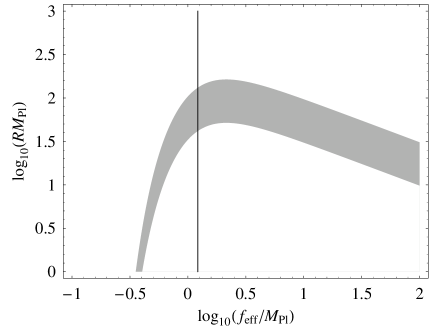
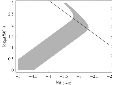
Figure 1: The plot of $\mathcal{P}_{\mathcal{R}}^{1/2}$ in the (left) $f_{\rm eff}/M_{\rm Pl}-RM_{\rm Pl}$ and (right) $g_{\rm 4D}-RM_{\rm Pl}$ planes evaluated at $N=60$. The shaded regions denote $10^{-5}\lesssim\mathcal{P}_{\mathcal{R}}^{1/2}\lesssim 10^{-4}$, and the solid lines correspond to $n_{\mathcal{R}}=0.96$. Note that while for a large region $n_{\mathcal{R}}$ is saturated at $n_{\mathcal{R}}\approx 0.967$ (see Eq. (37)), only a limited region is allowed for $\mathcal{P}_{\mathcal{R}}^{1/2}$.

		$\mathcal{P}_{\mathcal{R}}^{1/2}$	$n_{\mathcal{R}}$	$r$
$\log_{10}(f_{\rm eff}/M_{\rm Pl})=0.00$	analytic	$4.96\times 10^{-5}$	0.952	0.032
$\log_{10}(RM_{\rm Pl})=2.04$	numerical	$4.84\times 10^{-5}$	0.955	0.033
$\log_{10}(f_{\rm eff}/M_{\rm Pl})=0.50$	analytic	$1.25\times 10^{-5}$	0.967	0.117
$\log_{10}(RM_{\rm Pl})=2.04$	numerical	$1.33\times 10^{-5}$	0.967	0.112
$\log_{10}(f_{\rm eff}/M_{\rm Pl})=1.00$	analytic	$3.94\times 10^{-5}$	0.967	0.131
$\log_{10}(RM_{\rm Pl})=1.54$	numerical	$4.25\times 10^{-5}$	0.967	0.130
$\log_{10}(f_{\rm eff}/M_{\rm Pl})=1.50$	analytic	$1.25\times 10^{-5}$	0.967	0.131
$\log_{10}(RM_{\rm Pl})=1.54$	numerical	$1.33\times 10^{-5}$	0.967	0.112
$\log_{10}(f_{\rm eff}/M_{\rm Pl})=2.00$	analytic	$3.94\times 10^{-5}$	0.967	0.132
$\log_{10}(RM_{\rm Pl})=1.04$	numerical	$4.26\times 10^{-5}$	0.967	0.134

Table 1: From the top row, $R$ is chosen to make the inflationary energy scale $\Lambda=10^{-3}M_{\rm Pl}$, $10^{-5/2}M_{\rm Pl}$ and $10^{-2}M_{\rm Pl}$. Also note that $r$ is fairly close to the observational sensitivity of near future experiments. As can be seen from this table, the leading approximation of taking $n=1$ piece of Eq. (17) is reasonably good.

From Eqs. (29), (30) and (31), we can see that $n_{\mathcal{R}}$, $r$ and $f_{\mathrm{NL}}$ are dependent only on the effective decay constant $f_{\rm eff}$. This leads to the following simple expressions in the limit $f_{\rm eff}/M_{\rm Pl}\to\infty$, which is favored for long enough inflation, as

$$n_{\mathcal{R}}\approx 1-\frac{4}{1+2N}\,,$$ (37)

$$r\approx \frac{16}{1+2N}\,,$$ (38)

$$-\frac{3}{5}f_{\mathrm{NL}}\approx \frac{2+f_{k}}{2(1+2N)}\,,$$ (39)

respectively. Thus we can see that in this limit, evaluated at a certain $e$-folds before the end of inflation, they have definite values independent of $f_{\rm eff}$ or $R$. This is not surprising: huge $f_{\rm eff}$ means that the total number of $e$-folds we can obtain is enormous, and the last 60 $e$-folds is only a final tiny fraction of the whole expansion. Therefore the physical properties at this moment become completely insensitive to the detail of the model, since already the inflationary dynamics is following the late time attractor. It is this reason why we obtain almost identical values of $n_{\mathcal{R}}$, $r$ and $f_{\mathrm{NL}}$ in the limit $f_{\rm eff}/M_{\rm Pl}\to\infty$. This also means that the shape of $\mathcal{P}_{\mathcal{R}}$ is identical, meanwhile only its overall amplitude does depend on the inflationary energy scale.

We show the $r-n_{\mathcal{R}}$ plot in Fig. 2. Note that as shown in Eqs. (37) and (38), they are saturated as $f_{\rm eff}/M_{\rm Pl}\to\infty$, which corresponds to the upper right end of the curve where $n_{\mathcal{R}}\approx 0.967$ and $r\approx 0.132$. The shaded region shows the current observational $1\sigma$ bound $n_{\mathcal{R}}=0.960^{+0.014}_{-0.013}$ which is derived from the WMAP 5-year data combined with the observations of the type Ia supernovae (SN) and the baryon acoustic oscillations (BAO) [5], and the points on the curve explicitly denote several constraints on $n_{\mathcal{R}}$: the central value $n_{\mathcal{R}}=0.960$ (circle), and the lower bound $n_{\mathcal{R}}^{\rm lower}=0.947$ (triangle). Our model is well below the upper bound $n_{\mathcal{R}}^{\rm upper}=0.974$ (square) and there is no solution which corresponds to this point. The corresponding values of $r$ are 0.0528 and 0.0230, respectively. The current upper limit $r<0.20$ (95% confidence level) encompasses the whole predicted range of $r$ of our model. For the observationally allowed range of $n_{\mathcal{R}}$, $0.01\lesssim r\lesssim 0.1$ and is large enough to be detected within a few years by the forthcoming cosmological experiments and therefore may serve as the first observational test. Also note that $|f_{\mathrm{NL}}|$ is always much smaller than 1 and hence non-Gaussian signature is absolutely not observable at all.

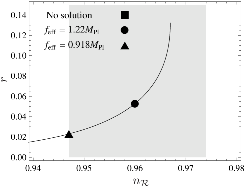
Figure 2: The prediction of the model in the $r-n_{\mathcal{R}}$ plane. Both $r$ and $n_{\mathcal{R}}$ are evaluated at 60 $e$-folds before the end of inflation. The shaded region shows the current observational $1\sigma$ bound derived from the WMAP 5-year + SN + BAO data: $n_{\mathcal{R}}=0.960^{+0.014}_{-0.013}$. Our model is well within the observational upper abound and has a large range of parameter space satisfying the lower bound.

After inflation ends, the inflaton starts oscillation at the global minimum. Although we are assuming no direct coupling between the hidden and the visible sectors, they can communicate gravitationally and the energy stored in the inflaton field can be converted to the light relativistic particles of the standard model to reheat the universe. Let us estimate the reheating temperature $T_{\mathrm{RH}}$ via the gravitational interaction in terms of the parameters of our model. With the interaction rate

$$\Gamma_{\mathrm{grav}}\sim\frac{m_{\phi}^{3}}{M_{\rm Pl}^{2}}\,,$$ (40)

using

$$m_{\phi}^{2}\sim V^{\prime\prime}\sim\frac{1}{f_{\rm eff}^{2}R^{4}}=\frac{M_{\rm Pl}^{2}}{(f_{\rm eff}/M_{\rm Pl})^{2}(RM_{\rm Pl})^{4}}\,,$$ (41)

we can write Eq. (40) as

$$\Gamma_{\mathrm{grav}}\sim\frac{M_{\rm Pl}}{(f_{\rm eff}/M_{\rm Pl})^{3}(RM_{\rm Pl})^{6}}\,.$$ (42)

From the fact that inflation ends when $\dot{\phi}_{\mathrm{end}}^{2}=V_{\mathrm{end}}$, we can find the Hubble parameter at the end of inflation, under the approximation Eq. (18), as

$$H_{\mathrm{end}}= \frac{3}{(2\pi)^{3/2}\pi}(RM_{\rm Pl})^{-1}\left[16\pi(f_{\rm eff}/M_{\rm Pl})^{2}+1\right]^{-1/2}R^{-1}$$

$$\sim \mathcal{O}(0.1)\frac{R^{-1}}{(f_{\rm eff}/M_{\rm Pl})RM_{\rm Pl}}\,.$$ (43)

Thus, for most parameter space $H_{\mathrm{end}}\gg\Gamma_{\mathrm{grav}}$ and the energy transfer occurs well after inflation. We can now easily see that the reheating temperature $T_{\mathrm{RH}}$ is estimated to be [21]

$$T_{\mathrm{RH}}\lesssim\mathcal{O}(0.1)\sqrt{\Gamma_{\mathrm{grav}}M_{\rm Pl}}\sim\mathcal{O}(0.1)\frac{M_{\rm Pl}}{(f_{\rm eff}/M_{\rm Pl})^{3/2}(RM_{\rm Pl})^{3}}\,.$$ (44)

As an example, if we put $f_{\rm eff}/M_{\rm Pl}=1$ and $RM_{\rm Pl}=100$, the maximum reheating temperature is estimated to be $T_{\mathrm{RH}}\sim 10^{12-13}\mathrm{GeV}$. The universe then follows the well known hot big bang evolution.

4 Conclusions

In this paper, we have presented a cosmological scenario from the hidden sector $SU(2)$ gauge symmetry in the five dimensional orbifold $M_{4}\times S^{1}/\mathbb{Z}_{2}$. The model is minimal in several aspects: the minimal non-Abelian gauge group and the minimal orbifold compactification with the minimal number of extra dimensions. Thanks to the non-Abelian nature, the bulk gauge boson, the fifth component $A_{5}$ in particular, could have a one-loop induced effective potential without introducing any exotic field in the model. This makes sure the minimality of the model. The advantage of this minimal setup is as follows: the inflaton field is a built-in ingredient of the theory and is automatically free from quantum gravitational effects because of its higher dimensional locality and the gauge symmetry. Fully radiatively generated one-loop potential is naturally able to support a long enough period of slow-roll inflation provided that the theory is weakly coupled, i.e. $g_{\rm 4D}\ll 1$, during the inflationary epoch. In very good numerical precision, the minimal model essentially provides a realization of natural inflation

$$V(\phi)\approx\Lambda^{4}\left[1-\cos\left(\frac{\phi}{f_{\rm eff}}\right)\right]\,,$$ (45)

with $\Lambda^{4}=9R^{-4}/(2\pi)^{6}$ and $f_{\rm eff}=(2\pi g_{\rm 4D}R)^{-1}$. For $10\lesssim RM_{\rm Pl}\lesssim 100$ and $1\lesssim f_{\rm eff}/M_{\rm Pl}\lesssim 100$, the model predicts the observable cosmological quantities

$$1.2\times 10^{-5}\lesssim\mathcal{P}_{\mathcal{R}}\lesssim 4.9\times 10^{-5}\,,$$ (46)

$$0.952\lesssim n_{\mathcal{R}}\lesssim 0.966\,,$$ (47)

$$0.03\lesssim r\lesssim 0.13\,.$$ (48)

The power spectrum of the curvature perturbation $\mathcal{P}_{\mathcal{R}}$ and the corresponding spectral index $n_{\mathcal{R}}$ are in good agreement with the current observations. While $|f_{\mathrm{NL}}|$ is always far smaller than 1 and no detectable non-Gaussianity is expected, very interestingly the predicted tensor-to-scalar ratio $r$ is quite close to sensitivity of the near future cosmological experiments. This would be the first test of our minimal cosmological model. The reheating temperature $T_{\mathrm{RH}}$ is estimated to be high enough to successfully follow the standard hot big bang evolution.

Acknowledgements

We are grateful to Misao Sasaki and the Yukawa Institute for Theoretical Physics at Kyoto University where some part of this work was carried out during “Scientific Program on Gravity and Cosmology” (YITP-T-07-01) and “KIAS-YITP Joint Workshop: String Phenomenology and Cosmology” (YITP-T-07-10). JG thanks Daniel Chung, L. Sriramkumar and Ewan Stewart for helpful conversations, and is partly supported by the Korea Research Foundation Grant KRF-2007-357-C00014 funded by the Korean Government. SCP appreciates Yasunori Nomura for his comments on low energy constraints of $g_{\rm 4D}$ and also thanks C. S. Lim for encouragement to publish this paper.

References

- [1] A. H. Guth, Phys. Rev. D 23, 347 (1981) ; A. D. Linde, Phys. Lett. B 108, 389 (1982) ; A. Albrecht and P. J. Steinhardt, Phys. Rev. Lett. 48, 1220 (1982).
- [2] See, e.g. A. R. Liddle and D. H. Lyth, “Cosmological inflation and large-scale structure,” Cambridge, UK: Univ. Pr. (2000) 400 p ; V. Mukhanov, “Physical foundations of cosmology,” Cambridge, UK: Univ. Pr. (2005) 421 p.
- [3] See, e.g. D. H. Lyth and A. Riotto, Phys. Rept. 314, 1 (1999) [arXiv:hep-ph/9807278].
- [4] M. Tegmark et al. [SDSS Collaboration], Phys. Rev. D 69, 103501 (2004) [arXiv:astro-ph/0310723] ; U. Seljak et al. [SDSS Collaboration], Phys. Rev. D 71, 103515 (2005) [arXiv:astro-ph/0407372] ; D. N. Spergel et al. [WMAP Collaboration], Astrophys. J. Suppl. 170, 335 (2007) [arXiv:astro-ph/0603449].
- [5] E. Komatsu et al. [WMAP Collaboration], arXiv:0803.0547 [astro-ph].
- [6] E. J. Copeland, A. R. Liddle, D. H. Lyth, E. D. Stewart and D. Wands, Phys. Rev. D 49, 6410 (1994) [arXiv:astro-ph/9401011].
- [7] K. Freese, J. A. Frieman and A. V. Olinto, Phys. Rev. Lett. 65, 3233 (1990) ; F. C. Adams, J. R. Bond, K. Freese, J. A. Frieman and A. V. Olinto, Phys. Rev. D 47, 426 (1993) [arXiv:hep-ph/9207245].
- [8] N. Arkani-Hamed, H. C. Cheng, P. Creminelli and L. Randall, Phys. Rev. Lett. 90, 221302 (2003) [arXiv:hep-th/0301218].
- [9] D. E. Kaplan and N. J. Weiner, JCAP 0402, 005 (2004) [arXiv:hep-ph/0302014].
- [10] S. C. Park, JCAP 11, 001 (2007) arXiv:0704.3920 [hep-th].
- [11] M. Kubo, C. S. Lim and H. Yamashita, Mod. Phys. Lett. A 17, 2249 (2002) [arXiv:hep-ph/0111327].
- [12] G. Cacciapaglia, C. Csaki and S. C. Park, JHEP 0603, 099 (2006) [arXiv:hep-ph/0510366].
- [13] N. Haba, Y. Hosotani and Y. Kawamura, Prog. Theor. Phys. 111, 265 (2004) [arXiv:hep-ph/0309088].
- [14] J. O. Gong and E. D. Stewart, Phys. Lett. B 510, 1 (2001) [arXiv:astro-ph/0101225].
- [15] E. Komatsu and D. N. Spergel, Phys. Rev. D 63, 063002 (2001) [arXiv:astro-ph/0005036].
- [16] J. M. Maldacena, JHEP 0305, 013 (2003) [arXiv:astro-ph/0210603].
- [17] S. Dodelson and E. Stewart, Phys. Rev. D 65, 101301 (2002) [arXiv:astro-ph/0109354] ; E. D. Stewart, Phys. Rev. D 65, 103508 (2002) [arXiv:astro-ph/0110322] ; J. Choe, J. O. Gong and E. D. Stewart, JCAP 0407, 012 (2004) [arXiv:hep-ph/0405155].
- [18] J. O. Gong, arXiv:0710.3835 [astro-ph].
- [19] N. Arkani-Hamed, L. Motl, A. Nicolis and C. Vafa, JHEP 0706, 060 (2007) [arXiv:hep-th/0601001].
- [20] J. O. Gong, Phys. Rev. D 75, 043502 (2007) [arXiv:hep-th/0611293].
- [21] See, e.g. A. D. Linde, “Particle physics and inflationary cosmology,” Chur, Switzerland: Harwood (1990) 362 p.