Supercooling and the Metal-Insulator Phase Transition of NdNiO₃

Abstract

We report the temperature and time dependence of electrical resistivity on high temperature, high oxygen pressure prepared polycrystalline samples of NdNiO₃. NdNiO₃ is metallic above 195 K and below that temperature it undergoes a transition to an insulating state. We find that on cooling NdNiO₃ below 195 K it goes into a state which is not in thermodynamic equilibrium and slowly relaxes over several hours. As we cool it further and go below about 110 K it goes into a stable insulating state. On heating the system from the insulating state towards 200 K we find that it remains stable and insulating and undergoes a rather sharp insulator to metal transition in the temperature range 185 K to 195 K. We try to make sense of these and a few other interesting observations on the basis of our current understanding of first order phase transitions, supercooling, and metal-insulator transitions.

I INTRODUCTION

Rare earth nickelates with the chemical formula RNiO₃, where R stands for a rare earth ion, is one of the few families of oxides that undergoes a first order metal-insulator phase transition. A metal-insulator transition (M-I transition) is an electronic phase transition which is usually solid to solid. The first order electronic phase transition in many systems is associated with a hysteresis, and they exhibit a phase separated (PS) state in the vicinity of the transition (Granados_1, ; Chen, ; Chaddah, ). The PS state has drawn a lot of attention in the case of manganites, mainly due to its implications for colossal magnetoresistance, and it exhibits a variety of time dependent effects such as relaxation of resistivity (Chen, ; Levy, ) and magnetization (Ghivelder, ) and giant 1/f noise (Podzorov, ).

RNiO₃ crystallizes in the orthorhombically distorted perovskite structure with space group P_bnm. The degree of distortion increases with decrease in size of rare earth ion as one moves towards the right in the periodic table (Medarde, ). The ground state of nickelates (R $\neq$ La) is insulating and antiferromagnetic. On increasing the temperature these compounds undergo a temperature driven antiferromagnetic to paramagnetic transition, and an insulator to metal transition. For NdNiO₃ and PrNiO₃, the M-I transition temperature ($T_{MI}$) and the magnetic ordering temperature ($T_{N}$) are the same, while $T_{MI}$ is greater than $T_{N}$ for later members of the series such as EuNiO₃ and SmNiO₃. The $T_{MI}$ of nickelates increases with decreasing size of the rare earth ion and the later members of the series also show a charge ordering transition associated with the M-I transition Medarde ; Alonso_1 ; Alonso_2 . The charge ordered state has also been observed in epitaxially grown thin films of NdNiO₃(Staub, ).

The M-I transition in NdNiO₃ is associated with a latent heat and a sudden increase in unit cell volume which are signatures of a first order phase transitionGranados ; Torrance . There is also a hysteresis in electronic transport properties just below $T_{MI}$ (Granados, ). The hysteresis in transport measurements points toward the coexistence of metallic and insulating phases below $T_{MI}$ Granados . In this paper we report a detailed study of the nature of NdNiO₃ below $T_{MI}$ through temperature and time dependent electrical resistivity measurements.

II EXPERIMENTAL DETAILS

Polycrystalline NdNiO₃ samples in the form of 6 mm diameter and 1 mm thick pellets were prepared and characterized as described elsewhere(Lcorre, ). The preparation method uses a high temperature of 1000^∘C and a high oxygen pressure of 200 bar.

All the temperature and time dependent measurements were done in a home made cryostat. To avoid thermal gradients in the sample during measurement it was mounted inside a thick-walled copper enclosure so that during the measurement the sample temperature would be uniform. It was found that mounting the sample like this improved the reproducibility of the data, especially in the time dependence measurements, significantly. A Lakeshore Cryotronics temperature controller model 340 was used to control the temperature and the temperature stability was found to be better than 3 mK during constant temperature measurements.

Below $T_{MI}$ NdNiO₃ is not in thermodynamic equilibrium and slowly relaxes. Because of this the data we get depend on the procedure used for the measurement. We used the following procedure to measure the temperature dependence of resistivity. While cooling we start from 300 K, and then record the data in steps of 1 K interval after allowing the temperature to stabilize at each point. In between two temperature points the sample was cooled at a fixed cooling rate of 2 K/min. After the cooling run is over we wait for one hour at 82 K and then the heating data was collected at every one degree interval. The intermediate heating rate between temperature points was the same as the cooling rate used earlier. This cycle of measurements was repeated with a different cooling and heating rate of 0.2 K/min also.

It was observed that the resistivity above $T_{MI}$ does not show any time dependence, and it is also independent of measurement history. Thus to avoid the effect of any previous measurements, all time dependent experiments in the cooling run were done as follows: first take the sample to 220 K (above $T_{MI}$), wait for half an hour, then cool at 2.0 K/min to the temperature of interest and once the temperature has stabilized record the resistance as a function of time. In the heating run the time dependent resistivity was done in a similar fashion: first take the sample to 220 K, wait for half an hour, then cool at 2.0 K/min to 85 K, wait for one hour, and then heat at 2.0 K/min to the temperature of interest and once the temperature has stabilized record the resistance as a function of time.

The four probe van der Pauw method was used to measure the resistivity and standard precautions, such as current reversal to take care of stray emfs, were taken during the measurement. We also took care to ensure that the measuring current was not heating up the sample. A Keithley current source model 224 and a DMM model 196 were used for the resistivity measurements.

III RESULTS

Figure

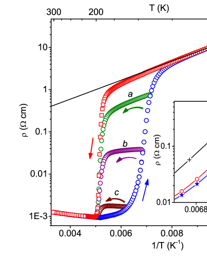
Figure 1: (Color online) $\rho$ vs. $1/T$ plot for NdNiO₃. The blue circles represent cooling data and the red squares stand for heating data (cooling/heating rate 2.0 K/min). The solid line is a least square fit to the band gap insulator model below 115 K. The curves labeled a, b & c were taken as described in the text. The accuracy of the data points is better than 1% everywhere. The error does not exceed 0.8 m$\Omega$cm anywhere. The inset shows $\rho$ vs $1/T$ for three different cooling rates: lower curve (blue stars): 2 K/min, middle curve (red circles): 0.2 K/min, upper curve (black pluses): infinitely slowly (explained in text). The connecting lines are to guide the eyes.

1 shows the electrical resistivity of NdNiO₃ as a function of temperature. We see that the function is multiple valued, the cooling and heating data differing significantly from each other and forming a large hysteresis loop. The resistivity plot indicates that NdNiO₃ undergoes a relatively sharp M-I transition at about 190 K while heating with a width of about 10 K. In contrast, while cooling, the resistivity shows a rather broad M-I transition centered around 140 K with a spread of about 40 K. Below 115 K or so, the heating and cooling data merge and the $\log\rho$ vs $1/T$ plot is linear. This indicates that the sample is insulating at low temperatures and, if the band gap is $\Delta$, the resistivity should follow the relation

$$\rho(T)=\rho_{0}\exp(\Delta/k_{B}T)$$ (1)

Below 115 K the data fit quite well to this model, with a coefficient of determination, $R^{2}$= 0.99955. $\rho_{0}$ and $\Delta$ for the insulating region turn out to be 99 m$\Omega$ cm and 42 meV respectively, which are in reasonable agreement with the values previously reported(Granados, ).

We collected more hysteresis data with different minimum temperatures such as 140 K, 146 K and 160 K. In these measurements we cool the sample from 220 K to one of the minimum temperatures mentioned above and then heat it back to 220 K, both operations being carried out at a fixed rate of 2 K/min. Loops formed in this fashion are called minor loops and these are indicated by the labels a, b and c in Figure 1. In the cooling cycle all the three minor loops coincide with the cooling curve of the full hysteresis loop. In the heating cycle, for loops a and b with lower minimum temperatures, the resistivity decreases with increasing temperature and joins the full loop at 195 K. In the case of loop c, as we increase the temperature, the resistivity increases somewhat till about 182 K and then it falls and joins the full loop at 195 K.

The resistivity also shows a noticeable dependence on the rate of temperature change in the cooling cycle as shown in the inset of Figure 1. The data for the lowest curve was collected at 2 K/min and for the middle curve at 0.2 K/min. The uppermost curve is an estimate obtained by extrapolating the time dependence data shown in Figure 2 to infinite time. We did not see any rate dependence in the heating cycle. This is an indication that while cooling, below the M-I transition temperature, the system is not in equilibrium and hence the resistivity evolves with time. The non-rate dependence observed in the data while heating tells us that in the heating cycle the system is either in, or very close to, equilibrium. These observations are corroborated by the data shown in Figure 2.

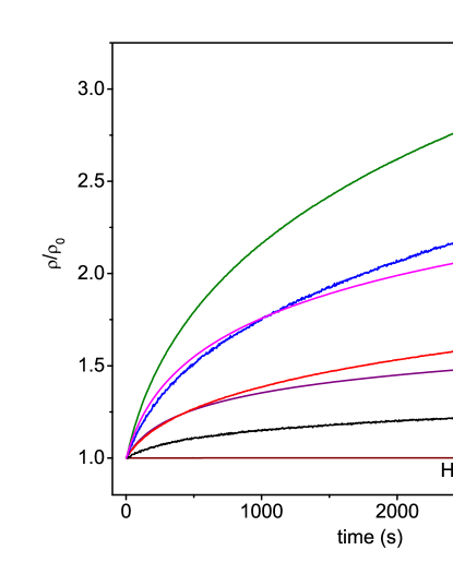
Figure 2: (Color online) Time dependence of resistivity while cooling, at various temperatures in the range 140 to 155 K, for a period of one hour. Maximum time dependence is seen at 145 K which is about 300 %. The curve at the bottom, which looks like a straight line, shows the increase in resistivity in a heating run taken at 145 K and the change in this case is less than 0.2 %. Not all the data are shown here to avoid clutter.

A subset of the time dependent resistivity data taken while cooling is shown in Figure 2. The data are presented as $\rho(t)/\rho(t=0)$ so that the values are normalized to unity at $t=0$ for easy comparison. We found that that below 160 K, the resistivity of the sample increases with time considerably. A maximum relative increase in resistivity of about 300 % for a duration of one hour is seen at 145 K, the time dependence being lower both above and below this temperature. We fitted the $\rho(T,t)$ curves in figure 2 to the stretched exponential function

$$\rho(t)=\rho_{0}+\rho_{1}(1-\exp(-(t/\tau)^{\gamma}))$$ (2)

where $\rho_{0}$, $\rho_{1}$, $\tau$ and $\gamma$ are fit parameters. The fits are quite good with the $R^{2}$ value greater than 0.999 in most cases. See Table 1. We note that the exponent $\gamma$ lies in the range $0.5<\gamma<0.6$ and $\tau$ has a peak around 147.5 K. The variation of resistivity with time shows that the system slowly evolves towards an insulating state at a constant temperature. We collected data up to 12 hours (not shown here) to check whether the system reaches an equilibrium state, but found that it was continuing to relax even after such a long time.

#	T(K)	$\rho_{1}/\rho_{0}$	$\tau$ ($10^{3}$s)	$\gamma$	$\chi^{2}/DOF$	$R^{2}$
1	140.0	0.764(5)	1.52(1)	0.538(3)	9.5	0.99971
2	142.5	1.89(1)	2.02(2)	0.554(2)	5.9	0.99981
3	145.0	4.59(3)	5.05(5)	0.567(1)	0.67	0.99993
4	147.5	3.39(6)	7.9(3)	0.568(3)	0.51	0.99978
5	150.0	1.22(1)	4.04(6)	0.582(2)	0.0014	0.99988
6	155.0	0.391(5)	2.6(1)	0.557(7)	0.0003	0.99845

Table 1: Fit parameters for the time dependence data shown in Figure 2. The degrees of freedom of the fits $DOF\approx 1000$. The $\chi^{2}/DOF$ for 150 K and 155 K are too small, indicating that we have overestimated the error in resistivity in these cases. Anyway, we note that, the $R^{2}$ values are consistently good and indicate reasonably good fits.

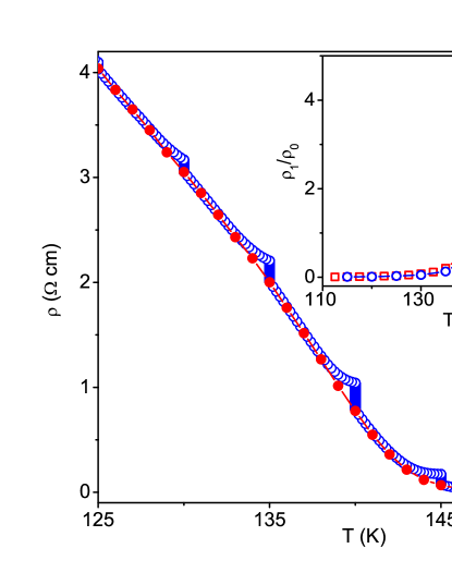
Figure 3: (Color online) Temperature dependence of $\rho$ on cooling with ageing by intermediate stops of one hour each (blue open circles) at 155, 150, 145, 140, 135, and 130 K. Red solid circles show the resistivity without ageing. The inset compares the temperature dependence of $\rho_{1}/\rho_{0}$ calculated from the fit of Equation (2) to $\rho(T,t)$ data with intermediate ageing (blue circles) to the time dependence data shown in Figure 2(red squares).

Figure 3 compares the resistivity in a cooling run with and without intermediate aging. These data were taken as follows: we start from 220 K, come down to 160 K at 2 K/min, collect time dependence data for one hour and after that resume cooling at 2 K/min and go down to 155 K, collect resistivity time dependence again for one hour and so on down to 110 K for every 5 K interval. We note that when cooling is resumed after aging for an hour, $\rho(T)$ curve merges smoothly with the curve obtained without aging. A rather similar observation has been reported in the phase-separated manganite La_0.5Ca_0.5Mn_0.95Fe_0.05O₃ (Levy, ).

The red squares in the inset of Figure 3 displays $\rho_{1}/\rho_{0}$ obtained from stretched exponential fitting of time dependence resistivity data of Figure 2. The $\rho_{1}/\rho_{0}$ increases on decreasing the temperature below 160 K, attains a maximum around 145 K, and then decreases on further lowering the temperature. We have already seen this behavior in Table 1. The value of $\rho_{1}/\rho_{0}$ obtained from the fitting of time dependence data with intermediate aging is shown as blue circles in the inset of figure 3, and we note that the value of $\rho_{1}/\rho_{0}$ is relatively small compared to what one obtains without intermediate aging.

In the heating cycle, the $\rho$ vs $T$ exhibits a rather sharp insulator to metal transition. The magnitude of time dependence in heating runs (maximum $\approx 0.2\%$) is negligible compared to what one gets in cooling runs (maximum$\approx 300\%)$ (figure 2), which suggest that in the heating run, below $T_{MI}$, the sample is almost fully insulating and stable.

The major observations that have been made so far are summarized below.

1. The metal to insulator transition in cooling runs is rather broad and extends from about 160 K to 120 K.

2. In cooling runs a large amount of time dependence in resistivity is seen compared to which the time dependence seen in heating runs is negligible.

3. NdNiO₃ undergoes a rather sharp insulator to metal transition between 185K and 195 K while heating.

4. There is a large hysteresis between the cooling and heating data below the MI transition temperature.

IV DISCUSSION

It has been known that the M-I transition in NdNiO₃ is associated with a latent heat and a jump in the unit cell volume which are the characteristics of a first order phase transitionTorrance ; Granados . DSC measurements of Granados et al. show that, while cooling, the latent heat released during the M-I transition extends over a broad temperature range(Granados, ). This is consistent with the results of the resistivity measurements that the M-I transition in NdNiO₃ is broadened while cooling . Thus we can say that NdNiO₃ has a broadened first order metal to insulator phase transition while cooling.

We have seen that, below $T_{MI}$, while cooling, the system is not in equilibrium and evolves with time which suggests that it is in a metastable state. The resistivity of this metastable state slowly increases with time which means that a slow metal to insulator transition is going on in the system. On the other hand while heating up from low temperature we saw that the system remains insulating all the way up to 185 K and then it transitions to the metallic state by 195 K. The resistivity was found to have negligible time dependence during the whole of the heating run. This result indicates that the low temperature insulating state is stable and is probably the ground state of the system. It is well known that below a phase transition temperature a high temperature phase can survive as a metastable supercooled state. Based on these facts we propose that the metastable state in the case of NdNiO₃ consists of supercooled (SC) metallic phases and stable insulating phases.

In a first order transition, a metastable SC phase can survive below the first order transition temperature ($T_{C}$), till a certain temperature called the limit of metastability ($T^{*}$) is reached Chaikin (15, , 14). In the temperature range $T^{*}<T<T_{C}$ there is an energy barrier separating the SC phase from the stable ground state. The height of the energy barrier ($U$) separating the SC metastable phase from the stable ground state can be written as $U\propto f(T-T^{*})$, where $f$ is a continuous function of ($T-T^{*}$), and vanishes for $T\leq T^{*}$. As the temperature is lowered, at $T=T^{*}$, the SC metastable phase becomes unstable and switches over to the stable ground state (Chaikin, 15). At $T>T^{*}$ the SC metastable phase can cross over to the stable ground state with a probability (p) which is governed by the Arrhenius equation

$$p\propto exp(-U/\mbox{k}_{B}T)$$ (3)

which tells us that the barrier will be crossed with an ensemble average time constant $\tau\propto 1/p$. If we imagine an ensemble of such SC phases with the same barrier $U$, then the volume of the metastable phase will exponentially decay with a time constant $\tau$.

The energy barrier $U$ that we talked about in the previous paragraph is an extensive quantity. Our system is polycrystalline, ie., it is made up of tiny crystallites of different sizes. Each one of the crystallites will have an energy barrier proportional to its volume. Thus for a crystallite the energy barrier separating the metastable state from the ground state can be written as

$$U\propto Vf(T-T^{*})$$ (4)

where $V$ is the volume of the crystallite. As already mentioned $f$ is a continuous function which vanishes for non-positive values of its argument. This means that various crystallites with the same $T^{*}$ will have different energy barriers depending on their size which implies that the time constant $\tau$, of the previous paragraph, will spread out and become a distribution of time constants depending on the distribution of the size of the crystallites. This can give rise to the volume of the metallic state decaying in a stretched exponential manner with timePalmer (16, 17). This behavior of the metallic volume with time will give rise to the resistivity also evolving with time in a similar fashion. We shall see later in the discussion how the metallic volume, the resistivity, and their time dependences are connected with each other.

Imry and Wortis have argued that a weak disorder can cause a distribution of $T^{*}$’s in different regions of a sampleImry (18, ). This has been experimentally observed in a vortex lattice melting experiment in a high $T_{C}$ superconductor Soibel (19). In our case grain boundaries, shape of the crystallite etc. could be sources of disorder which would give rise to different $T^{*}$’s for different crystallites. This effect will further broaden the distribution of time constants in our system which arise from the distribution of crystallite sizes.

Coming back to the heating runs we note that the lack of time dependence of the resistivity data indicates that the system is in a stable state. Now the question arises: what is the reason for the width of about 10 K observed in the insulator to metal transition? Could it be a superheating effect? It cannot be because, as already noted, the lack of time dependence during heating runs rules out the possibility of any metastable phase in the system. The broadening while heating is most likely caused by the rounding of the phase transition due to finite size of the crystallites. A similar observation on broadening of phase transitions due to finite size of grains have been reported in a CMR manganiteFu (20).

Now we understand the reason for the hysteresis seen in this system. During a heating run from low temperature the system is insulating and hence its resistivity is high. While cooling some of the crystallites transform themselves into the stable insulating state while others remain in the supercooled metallic state . The presence of the metallic crystallites lowers the resistivity of the system. Thus we get different values of resistivity during heating and cooling runs giving rise to hysteresis in resistivity.

The picture so far: NdNiO₃ is polycrystalline and thus consists of tiny crystallites. Below $T_{MI}$, while cooling, the tiny crystallites can be in either a supercooled metallic state or a stable insulating state. A crystallite in the supercooled metallic state can make a transition to the stable insulating state if it crosses the barrier $U$ with the help of energy fluctuations which in our case are thermal in origin. Each crystallite would undergo the transition independent of each other. This is supported by the fact that the resistivity, and as we shall see later, the volume of the metastable metallic state, behave in a stretched exponential manner with time. At a particular temperature, as a function of time, the transition from the metallic to the insulating phase will begin with the smaller crystallites, because the barrier is small for them, and then proceed with the larger crystallites, in the increasing order of barrier size. While heating the system remains insulating and stable all the way up to the M-I transition and then it goes over to the stable metallic state. There is no superheating during heating runs.

Now that we have understood the origin of time dependence and hysteresis in the system we would like to consider some more issues that needs to be understood. These are

1. The dependence of resistivity on cooling rate as shown in the inset of Figure 1.

2. The behavior of the minor loops seen in Figure 1.

3. The intermediate ageing behavior seen in Figure 3.

4. Both $\rho_{1}/\rho_{0}$ and $\tau$ of Equation (2) go through a peak around 145 K and 147.5 K respectively as shown in Table 1 and also in the inset of Figure 3 and Figure 6.

Let us take up these issues one by one.

IV.1 Cooling Rate Dependence

In the inset of Figure 1 we saw that while cooling a lower cooling rate increases the resistivity of the sample in the hysteresis region. A lower cooling rate allows a larger number of the metastable metallic crystallites to switch over to the insulating state and thus the resistivity will be larger if the measurement is done slowly.

If the measurement is done infinitely slowly in the cooling run we should get the uppermost curve shown in the inset of Figure 1. It is interesting to note that this curve does not come anywhere near the heating run curve. To paraphrase, even if we sit for an infinite time on the cooling curve we cannot reach the heating curve. The reason for this is that only a small number supercooled crystallites which have a relatively small energy barrier are able to switch over to the insulating state at any given temperature. The others with the larger energy barriers remain trapped in the metallic state. These crystallites with the larger barriers can switch their state only if the temperature is lowered such that $T$ comes sufficiently close to $T^{*}$ and thus the barrier becomes small and easy to cross (Equation (4)).

IV.2 Minor Loops

The minor loops a, b, and c shown in Figure 1 follow the full hysteresis loop in the cooling cycle till we start the heating. While heating, curve a, with the lowest minimum temperature (140 K), shows a falling resistivity with increasing temperature. Curve b with the intermediate minimum temperature (146 K) shows a rather flat resistivity with increasing temperature, while curve c with the highest minimum temperature (160 K) shows a rising resistivity with increasing temperature initially before falling and joining the full hysteresis loop at the MI transition temperature 195 K.

The behavior of the minor loops can be understood by recognizing that the nature of resistivity, when heating is resumed, in the metastable region is determined by the competition between the temperature dependence and time dependence of resistivity. In the case of curve a, with the lowest minimum temperature, most of the crystallites will be in the insulating state as can be inferred from the large value of resistivity. Only few of the crystallites will be in the metastable state and hence the time dependence effects can be expected to be small. Thus during heating the resistivity of the sample will be dominated by the temperature dependence of resistivity of the insulating crystallites. This is the reason the heating part of the curve looks more or less parallel to the main heating curve before the onset of the transition.

The behavior of curve c is easier to understand and hence let us consider it before discussing curve b. In this case the resistivity is low and most of the crystallites are in the metallic state. The metallic crystallites form a percolating network and the resistivity of the sample will be governed by their behavior. The insulating crystallites are essentially shorted out and will have little role in determining the resistivity. The metallic crystallites, being metastable, will switch to the insulating state governed by Equation (3), thus slowly increasing the resistivity of the sample as a function of time. When the resistivity values are collected while heating, there will be some time difference between two data points depending on the heating rate, allowing a rise in resistivity to register. We would then find that the resistivity increases with increasing temperature. Curve b lies between curves a and c and in this case there will be a good number of both insulating and metallic crystallites. Here there would be competition between the temperature dependence of the insulating crystallites and the time dependence of the metallic crystallites and hence one can expect that the curve b would be more or less flat at the onset of heating.

IV.3 Intermediate Ageing

Now let us consider the intermediate ageing data shown in Figure 3. We note that after ageing for one hour, when the cooling is resumed, the slope of the the $\rho$ vs. $T$ curve is less in magnitude than for the curve obtained without ageing. When we stop the cooling and age the sample at a fixed temperature the supercooled metallic crystallites with relatively small $U$ will switch over to the insulating state. This decreases the number of crystallites in the metallic state and raises the resistivity. So now, when the cooling is resumed, the number of metallic crystallites which can switch to the insulating state would be less and hence the change in resistivity with temperature would be lower.

From Figure 3 it is clear that on resuming cooling after an intermediate stop of one hour the cooling curve merges with the curve obtained without ageing within about 3 K or less. As already noted in the previous paragraph when we stop the cooling and age the sample at a fixed temperature the supercooled metallic crystallites with relatively small $U$ will switch over to the insulating state. As can be inferred from Equation (4) those crystallites will have a small $U$ which have (i) their metastability temperature ($T^{*}$) close to their temperature ($T$) (ii) a small size. The major contributions to resistivity change will come from the relatively larger crystallites making the transition from the metallic state to the insulating state. In the light of this the merger of the cooling curves with and without ageing within a small temperature change of about 3 K means that most of the crystallites which undergo the transition from metal to insulator during ageing have their $T^{*}$ within a few kelvin of the temperature of the sample. We had already reached this conclusion earlier when we discussed the cooling rate dependence.

IV.4 Peaks in $\rho_{1}/\rho_{0}$ and $\tau$

We had noted earlier that both $\rho_{1}/\rho_{0}$ and $\tau$ go through peaks around 145 K and 147.5 K respectively. The peak in $\rho_{1}/\rho_{0}$ is not surprising because it shows up in a region of temperature in the cooling curve where the resistivity changes very fast with temperature. Thus one would expect that a large number of metastable crystallites are switching over to the insulating state near this region. Hence if a relaxation measurement is done here we should see the effect of a large number of crystallites transitioning to the insulating state as a peak in $\rho_{1}/\rho_{0}$. But the peak in $\tau$ at about 147.5 K is not that easily understood. To check whether this peak has anything to with percolation we should examine how the metallic and insulating volumes depend on temperature.

The conductivity of a phase separated system depends on the volume fraction of insulating and metallic phases, their geometries, distribution, and their respective conductivities ($\sigma_{I}$ and $\sigma_{M}$). McLachlan has proposed an equation based on a general effective medium (GEM) theory for calculating the effective electrical conductivity $\sigma_{E}$ of a binary MI mixture (McLachlan, 21), which is

$$(1-f)\frac{(\sigma_{I}^{1/t}-\sigma_{E}^{1/t})}{(\sigma_{I}^{1/t}+A\sigma_{E}^{1/t})}+f\frac{(\sigma_{M}^{1/t}-\sigma_{E}^{1/t})}{(\sigma_{M}^{1}/t+A\sigma_{E}^{1/t})}=0$$ (5)

where $f$ is the volume fraction of the metallic phases and $A=(1-f_{c})/f_{c}$, $f_{c}$ being the volume fraction of metallic phases at the percolation threshold, and $t$ is a critical exponent which is close to 2 in three dimensions (Herrmann, 22, 23). The constant $f_{c}$ depends on the lattice dimensionality, and for 3D its value is 0.16 (Efros, 24). The GEM equation has been successfully applied to a wide variety of isotropic, binary, macroscopic mixtures and it works well even in the percolation regime (McLachlan, 21, 23, 25).

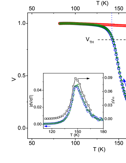
Figure 4: (Color online)Temperature variation of $V$ ($=1-f$), the insulating volume fraction. The blue circles show the cooling cycle (2 K/min cooling rate) and the red squares represent the heating cycle. The green pluses represent the insulating volume fraction for 0.2 K/min cooling rate. The dashed horizontal line at 84% insulating volume represents the percolation threshold. The inset shows the variation of $|dV/dT|$ (blue circles: cooling rate 2 K/min, and green pluses: cooling rate 0.2 K/min) and $\Delta V_{\infty}$ (black squares) with temperature.

In order to calculate the volume fraction of metallic and insulating phases from Equation (5), we need their respective resistivities $\rho_{M}(T)$ and $\rho_{I}(T)$. $\rho_{M}(T)$ was obtained using $\rho_{M}=\rho_{0}+AT$, where $A$ is the temperature coefficient of resistivity estimated from the resistivity data above the M-I transition. $\rho_{I}(T)$ was calculated using the parameters obtained by fitting the resistivity data below 115 K to Equation (1). Using the above information and the resistivity data, we calculated the volume fraction of metallic and insulating phases and it is shown in Figure 4. In the cooling cycle the volume fraction of the insulating phases ($V=1-f$) slowly increases on decreasing the temperature below $T_{MI}$, while in the case of heating cycle it remains nearly constant up to about 185 K, and then drops to zero by 200 K. As can be seen from Figure 4 the percolation threshold for the cooling runs occurs at around 144 K. Below this temperature there will be no continuous metallic paths in the system.

The rate of change of metallic volume fraction ($-dV/dT$) has a maximum around 147.5 K in the cooling runs (inset of Figure 4). Figure 5 displays the increment ($\Delta V$) of insulating volume fraction with time, that has been extracted from the time dependent resistivity data of Figure 2. Just as in the case of time dependence of resistivity, the $\Delta V(t)$ curves of Figure 5 were fitted to a stretched exponential function $\Delta V(t)=\Delta V_{\infty}(1-\exp(-(t/\tau)^{\gamma}))$, where the constant $\Delta V_{\infty}$ gives the increase in the insulating volume fraction when waiting for an infinitely long time. The inset of Figure 4 also shows the variation of $\Delta V_{\infty}$ with temperature, which mimics the behavior of $|dV/dT|$. Figure 6 compares the constant of relaxation $\tau$ obtained from the fitting of $\rho(t)$ and $\Delta V(t)$ curves of Figure 2 and 5 respectively. For the $\rho(t)$ curves, $\tau$ has a peak around 147.5 K while for the $\Delta V(t)$ curves, surprisingly, $\tau$ is nearly constant.

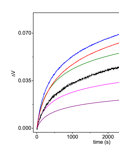
Figure 5: (Color online) Increase in volume fraction of insulating phases ($\Delta V$) with time, at various temperatures.

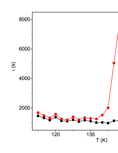
Figure 6: (Color online)Temperature variation of $\tau$ obtained from the stretched exponential fitting of $\rho(t)$ (red circles) and $\Delta V(t)$ (black squares) curves.

During cooling $|dV/dT|$ of the inset of Figure 4 represents the amount of volume that will change from the supercooled metallic to the insulating state for a unit temperature change. Now a small change in temperature will result in those supercooled crystallites with their $T^{*}$ falling in that temperature range switching to the insulating state. This means that the value of $|dV/dT|$ at $T$ is a good measure of the fraction of supercooled metastable crystallites which have their $T^{*}$ close to $T$. Thus $|dV/dT|$ of the cooling curve represents the distribution of $T^{*}$’s in the system. In coming to the above conclusion we have disregarded the small fraction of crystallites that would be switching due to the time elapsed in covering the small temperature change. This is supported by the fact that the $|dV/dT|$ values calculated from the 2 K/min and 0.2 K/min cooling curves are essentially the same.

The peak in $\triangle V_{\infty}$ occurs at 147.5 K which is also where the distribution of $T^{*}$’s peak. This is understandable because all the crystallites with $T^{*}$ close to 147.5 K would be switching to the insulating state if we wait for a sufficiently long time. Since the maximum number of crystallites with $T^{*}$ are close to 147.5 K, we will get the maximum temperature dependence for $\triangle V_{\infty}$ at 147.5 K.

One would have expected that the peak in $\rho_{1}/\rho_{0}$ and $\triangle V_{\infty}$ would occur at the same temperature. The peak in $\rho_{1}/\rho_{0}$ is at 145 K which is 2.5 K below the peak of $\triangle V_{\infty}$. The reason for this is that the resistivity would change faster for a given metallic volume change nearer the percolation threshold. We guess that even if the volume change is smaller at 145 K a larger resistivity change due to the proximity to the percolation threshold compensates for the smaller volume change and shifts the maximum of $\rho_{1}/\rho_{0}$ to that temperature.

As can be seen from Figure 6 the parameter $\tau$ of the resistivity time dependence fit has a peak around 147.5 K while there is no such peak in the $\tau$ of the volume fraction time dependence. The rather flat temperature dependence of the $\tau$ of the volume fraction is probably an indication that the distribution of energy barriers look more or less the same at all temperatures. We note that the difference in behavior of the $\tau$’s from resistivity and volume fraction is most pronounced close to the percolation threshold, while away from the threshold both $\tau$’s behave in a very similar manner. In a resistivity relaxation measurement, close to the percolation threshold, the resistivity will change significantly even when the metallic volume changes very little. Thus, one will find that, near the percolation threshold, the resistivity will relax over a longer time period.

V Conclusion

Our experimental results demonstrate that while cooling the physical state of NdNiO₃ is phase separated below the M-I transition temperature; the phase separated state consists of SC metallic and insulating crystallites. A metastable metallic crystallite switches from the metallic to the insulating state probabilistically depending on the closeness of the temperature of metastability and the size of the crystallite. At low temperature, below 115 K or so, the system is insulating, all the crystallites having switched over to the insulating state. While heating the crystallites remain in the stable insulating state till the MI transition temperature is reached and then they switch over to the metallic state.

- (1) X. Granados, J. Fontcuberta, X. Obradors, and J. B. Torrance, Phys. Rev. B 46, 15683 (1992)
- (2) X. J. Chen, H. -U. Habermier, and C. C. Almasan, Phys. Rev. B 68, 132407 (2003).
- (3) P. Chaddah, cond-mat/0109310v1
- (4) P. Levy, F. Parisi, L. Granja, E. Indelicato, and G. Polla, Phys. Rev. Lett. 89, 137001 (2002).
- (5) L. Ghivelder, F. Parisi, Phys. Rev. B 71, 184425 (2005).
- (6) V. Podzorov et al., Phys. Rev. B 61, R3784 (2000).
- (7) M. L. Medarde, J. Phys.: Condens. Matter 9, 1679 (1997).
- (8) J. A. Alonso et al., Phys. Rev Lett. 82, 3871 (1999).
- (9) J. A. Alonso et al., Phys. Rev. B 61, 1756 (2000).
- (10) U. Staub et al., Phys. Rev Lett. 88, 126402 (2002).
- (11) X. Granados et al., Phys. Rev. B 48, 11 666 (1993).
- (12) J. B. Torrance et al., Phys. Rev. B 45, 8209 (1992).
- (13) N. E. Massa, J. A. Alonso, M. J. Martinez-Lope, I. Rasines, Phys. Rev. B 56, 986 (1997).
- (14) P. Chaddah, and S. B. Roy, Phys. Rev. B 60, 11926 (1999).
- (15) P. M. Chaikin and T. C. Lubensky, Principles of Condensed Matter Physics (Cambridge University Press 1998) chapter 4.
- (16) R. G. Palmer, D. L. Stein, E. Abrahams and P. W. Anderson, Phys. Rev Lett. 53, 958 (1984).
- (17) M. D. Ediger, C. A. Angell, Sidney R. Nagel, J. Phys. Chem. 100, 13200 (1993).
- (18) Y. Imry, and M. Wortis, Phys. Rev. B 19, 3580 (1979).
- (19) A. Soibel et.al., Nature 406, 282 (2000).
- (20) Yonglai Fu, Appl. Phys. Lett., 77, 118 (2000).
- (21) D. S. McLachlan, J.Phys.C 20, 865 (1987).
- (22) H. J. Herrmann, B. Derrida, and J. Vannimenus, Phys. Rev. B 30, 4080 (1984).
- (23) G. Hurvits, R. Rosenbaum, and D. S. McLachlan, J. Appl. Phys. B 73, 7441 (1993).
- (24) A. L. Efros, Physics and Geometry of Disorder Percolation Theory (Mir Publishers Moscow 1986) chapter 6.
- (25) K. H. Kim, M. Uehara, C. Hess, P. A. Sharma, and S-W. Cheong, Phys. Rev Lett. 84, 2961 (2000).