Shot noise in a quantum dot coupled to non-magnetic leads: Effects of Coulomb interaction

Abstract

We study electron transport through a quantum dot, connected to non-magnetic leads, in a magnetic field. A super-Poissonian electron noise due to the effects of both interacting localized states and dynamic channel blockade is found when the Coulomb blockade is partially lifted. This is sharp contrast to the sub-Poissonian shot noise found in the previous studies for a large bias voltage, where the Coulomb blockade is completely lifted. Moreover, we show that the super-Poissonian shot noise can be suppressed by applying an electron spin resonance (ESR) driving field. For a sufficiently strong ESR driving field strength, the super-Poissonian shot noise will change to be sub-Poissonian.

1 Introduction

Shot noise, i.e., current fluctuations due to the discrete nature of electrons, describes the correlation in electron transport through mesoscopic systems, such as quantum dots (QDs) or molecular devices. Recently, shot noise measurements have provided additional information that is not available in conventional conductance measurements (for reviews, see Refs. [1] and [2]). In contrast to Poissonian noise often observed in classical transport, quantum transport of electrons is usually described by binomial statistics [3], as has been used to explain the suppression of noise in noninteracting conductors [4]. For quantum transport in many mesoscopic systems, the Coulomb repulsion allows an electron to enter a region only after the departure of another electron. This effect induces a negative electron correlation and, therefore, leads to a sub-Poissonian shot noise [5]. Instead of Coulomb blockade, an electron blockade due to the Pauli exclusion principle also has a similar effect [6]. Recently, it was found that the interplay between the Coulomb repulsion and Pauli-exclusion principle can lead to electron bunching, i.e., a super-Poissonian shot noise [7, 8].

There have been numerous theoretical studies on electron correlations [9, 10, 11, 12, 13, 14, 15, 16, 17, 18, 19, 20, 21]. Electron correlations in a single QD connected to two terminals have been studied theoretically in both sequential [9, 10, 11, 12] and coherent tunneling regimes [13, 14, 15]. A sub-Poissonian Fano factor of electrons transporting through two tunnel junctions was found to be due to a Coulomb blockade [9, 10]. In contrast, a super-Poissonian Fano factor has recently been predicted based on a dynamic channel blockade [11] which occurs when a QD is connected to spin polarized leads [12, 13] or is coupled to a localized level [14] at low temperature. In a three-terminal QD [16, 17], positive cross correlations have been obtained by lifting the spin degeneracy [17], comparing to the predicted intrinsic negative cross correlation when the level spacing of the dot is much smaller than thermal fluctuations [16]. Also, a super-Poissonian Fano factor has been found in the two-terminal case in the cotunneling regime [18, 19, 21].

Noise measurements have also been performed in many experimental realizations [7, 22, 23, 24, 25, 26, 27, 28]. The specific conditions under which super-Poissonian shot noise occur was investigated. Positive noise correlations due to the effect of interacting localized states [8] was observed in metal-semiconductor field transistors [7], mesoscopic tunnel barriers [22], and self-assembled stacked coupled QDs [23]. Dynamic channel blockade induced super-Poissonian shot noise has also been verified in both the weak tunneling [24, 25] and the quantum Hall regimes[26] in GaAs/AlGaAs QDs. In addition, positive cross correlations were also recently observed in an electronic beam splitter [27], as well as in capacitively coupled QDs [28].

Recently, Sánchez et al [29]. investigated the noise properties of electrons transporting through a QD containing two orbital levels. Only the case with at most one electron in the QD was considered. They found a super-Poissonian shot noise due to dynamic channel blockade. After applying an ac field to drive transitions between the two levels, the dynamic channel blockade is suppressed and the electron shot noise becomes sub-Poissonian at a large field strength. Also, Djuric et al [30]. considered the spin dependent transport of electrons through a QD with a single orbital level. Their results show that when the bias voltage is beyond that corresponding to the Coulomb blockade regime, the spin blockade is lifted and the spin-up and spin-down electrons can both tunnel through the QD independently. As a result, only a sub-Poissonian shot noise of electrons was obtained.

In the present work, we investigate the shot noise of electron transport through a single QD under a magnetic field. The QD is connected to two non-magnetic leads and can take a single-electron spin-up, single-electron spin-down or two-electron singlet states. In the nonequilibrium case, a bias voltage is applied and this leads to different chemical potentials in the two leads. Following a setup used to detect single-spin decoherence [31], there is a spin-dependent energy cost for adding a second electron into the QD, due to the effects of both Coulomb interactions and Zeeman splitting. If the left-lead chemical potential can supply the extra energy for only one of the spin orientations, the Coulomb blockade is partially lifted. In this regime, the transport mechanisms for the spin-up and spin-down electrons are different. Here, we also found a super-Poissonian shot noise, similar to that in [29], but it is caused by the effects of both interacting localized states and dynamic channel blockade is obtained. Moreover, we show that these effects can be suppressed by applying an electron spin resonance (ESR) driving magnetic field. When the ESR driving field is strong enough, the electron shot noise will change from super-Poissonian to sub-Poissonian.

The paper is organized as follows. In Sec. II, we introduce the theoretical model. The master equation and generating function are explained in Sec. III. Electron shot noise in the presence of an ESR magnetic field and couplings to the environment in various bias voltages are discussed in Sec. IV. Section V is a brief summary.

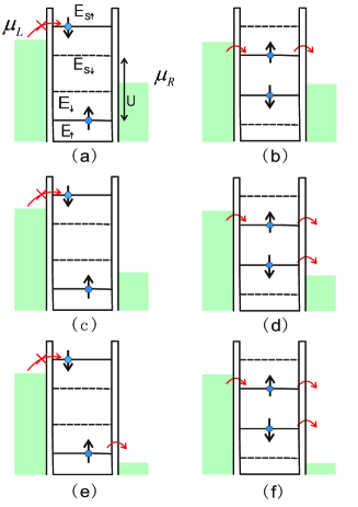
Figure 1: (Color online) Energy diagram of a QD connected to two non-magnetic leads with chemical potential $\mu_{L}$ and $\mu_{R}$, respectively. The left lead chemical potential is set between $E_{S\uparrow}$ and $E_{S\downarrow}$, i.e., $E_{S\uparrow}>\mu_{L}>E_{S\downarrow}$. By tuning the right lead chemical potential $\mu_{R}$, one can control the transport through the QD in three different regimes: (a) and (b) $E_{S\downarrow}>\mu_{R}>E_{\downarrow}$; (c) and (d) $E_{\downarrow}>\mu_{R}>E_{\uparrow}$; (e) and (f) $E_{\downarrow}>E_{\uparrow}>\mu_{R}$. The detailed transport mechanisms in these three regimes are explained in the text.

2 Theoretical model

We consider a single QD connected to two electron reservoirs by tunneling barriers, as schematically shown in Fig. 1. Electron transport can occur when there are discrete energy levels of the QD within the bias window defined by the chemical potentials $\mu_{L}$ and $\mu_{R}$ of the two leads. The full Hamiltonian reads

$$H\!=\!H_{\rm{leads}}+H_{\rm{dot}}+H_{\rm{T}},$$ (1)

with

$$H_{\rm{leads}}=\sum_{\alpha k\sigma}E_{\alpha k\sigma}c_{\alpha k\sigma}^{+}c_{\alpha k\sigma},$$ (2)

where $c_{\alpha k\sigma}^{+}$ ($c_{\alpha k\sigma}$) is the creation (annihilation) operator of an electron with momentum $k$ and spin $\sigma$ in lead $\alpha$ $(\alpha=l,r)$. $H_{\rm{dot}}$ represents the Hamiltonian of an isolated QD and is given by

$$H_{\rm{dot}}\!=\!\sum_{\sigma}E_{0\sigma}a_{\sigma}^{+}a_{\sigma}+Un_{\uparrow}n_{\downarrow}+H_{\rm{spin}},$$ (3)

where $E_{0\sigma}$ describes the orbital energy for the electron spin $\sigma$ and $U$ is the Coulomb interaction between electrons in the dot. We have defined $a_{\sigma}^{+}$ ($a_{\sigma}$) as the creation (annihilation) operator for electrons with spin $\sigma$, and $n_{\sigma}\!=\!a_{\sigma}^{+}a_{\sigma}$ is the number operator. External magnetic fields $B_{z}$ and $B_{x}$ are applied in the $z$ and $x$ directions, respectively. They result in an interaction $H_{\rm{spin}}$ given by

$$H_{\rm{spin}}\! \!=\! \!\frac{1}{2}[\Delta_{z}\sigma_{z}+\Delta_{x}\cos(\omega_{c}{t})\sigma_{x}],$$ (4)

where $\Delta_{z}\!=\!g\mu_{B}{B}_{z}$ and $\Delta_{x}\!=\!g\mu_{B}{B}_{x}$ with $g$ being the electron g factor, $\mu_{B}$ the Bohr magnetron and $\sigma_{z(x)}$ the Pauli operator. The first term in Eq. (4) generates a Zeeman splitting between two different spin states. The energy levels of these two spin states are $E_{\uparrow(\downarrow)}=E_{0}\mp\frac{1}{2}\Delta_{z}$. The second term in Eq. (4) is an ESR driving field with frequency $\omega_{c}$, which produces spin flips when it is resonant with the Zeeman splitting. The tunneling coupling between the QD and the leads is given by

$$H_{\rm{T}}=\sum_{k\sigma}(\Omega_{l}a_{\sigma}^{+}c_{lk\sigma}+\Omega_{r}a_{\sigma}^{+}c_{rk\sigma}+\rm{H.c.}),$$ (5)

where $\Omega_{l(r)}$ characterizes the coupling strength between the QD and the left (right) lead.

In the present discussion, only a single orbital level in the QD is considered. With one electron in the dot, it can be at either the spin-up ground state, $|\!\uparrow\rangle$, or the spin-down excited state, $|\downarrow\rangle$. When an additional electron enters the dot, we only need to consider the singlet ground state with two opposite spins, i.e., $|S\rangle=\frac{1}{\sqrt{2}}(|\uparrow\downarrow\rangle-|\downarrow\uparrow\rangle)$. This is because triplet states have symmetric spin wavefunctions. One of the electrons must then occupy a higher orbital level to attain an antisymmetric orbital wavefunction. In general, the energy difference between two orbital levels in a QD is much larger than the exchange energy between the spins. The triplet states can hence be neglected  [32, 33]. When the QD is occupied by one spin-up (down) electron, the energy cost $E_{S\uparrow(\downarrow)}$ to add a spin-down (up) electron to form a singlet state is $E_{S\uparrow(\downarrow)}=E_{\downarrow(\uparrow)}+U$ [31].

We first consider the case $E_{S\uparrow}>\mu_{L}>E_{S\downarrow}>\mu_{R}>E_{\downarrow}$, as shown in Figs. 1(a) and 1(b). From an initial spin-down state, a spin-up electron can enter the QD since $\mu_{L}>E_{S\downarrow}$. Moreover, for an initial spin-up state, the condition $E_{S\uparrow}>\mu_{L}$ implies that a second electron cannot enter the dot and the tunneling through the QD is blocked at low temperature. However, the QD becomes unblocked after exciting the electron spin via an ESR driving field (spin flips), but only a spin-up electron can tunnel into the QD from the left lead to form a singlet state. Then, either a spin-up or spin-down electron hops onto the right lead from this singlet state, leaving the QD in a single electron state again. In the intermediate regime with $E_{\downarrow}>\mu_{R}>E_{\uparrow}$ [see Figs. 1(c) and 1(d)], the transport mechanism is similar to that in the previous regime. The only difference is that a single spin-down electron in the dot can now hop onto the right lead, because $E_{\downarrow}>\mu_{R}$. Alternatively, when the right-lead chemical potential is further tuned down to the third regime with $\mu_{R}<E_{\uparrow}<E_{\downarrow}$, tunneling is always ensured, as shown in Figs. 1(e) and 1(f).

3 Master equation and generating function method

We have derived a particle number resolved master equation to describe the time evolution of the reduced density matrix, $\rho^{(m)}(t)$, of the QD [34]. The diagonal element $\rho_{ii}^{(m)}(t)$ $(i=0,\uparrow,\downarrow,S)$ gives the occupation probability of state $i$ assuming that $m$ electrons have arrived at the right lead at time $t$. The off-diagonal element $\rho_{\uparrow\downarrow}^{(m)}(t)$ describes the coherence of two spin states. In the Born-Markov approximation, the master equation [35, 36] is given, after some algebra, by

$$\dot{\rho}_{00}^{(m)}=-(W_{\uparrow 0}+W_{\downarrow 0})\rho_{00}^{(m)}+W_{0\uparrow}^{l}\rho_{\uparrow\uparrow}^{(m)}+W_{0\downarrow}^{l}\rho_{\downarrow\downarrow}^{(m)}+W_{0\uparrow}^{r}\rho_{\uparrow\uparrow}^{(m-1)}+W_{0\downarrow}^{r}\rho_{\downarrow\downarrow}^{(m-1)}$$

$$\dot{\rho}_{\uparrow\uparrow}^{(m)}=-(W_{S\uparrow}+W_{0\uparrow})\rho_{\uparrow\uparrow}^{(m)}+\gamma\rho_{\downarrow\downarrow}^{(m)}+W_{\uparrow S}^{l}\rho_{SS}^{(m)}+W_{\uparrow S}^{r}\rho_{SS}^{(m-1)}+W_{\uparrow 0}^{l}\rho_{00}^{(m)}+W_{\uparrow 0}^{r}\rho_{00}^{(m+1)}$$

$$+i\frac{\Omega}{2}(\rho_{\uparrow\downarrow}^{(m)}-\rho_{\downarrow\uparrow}^{(m)})$$

$$\dot{\rho}_{\downarrow\downarrow}^{(m)}\!=\!-(W_{S\downarrow}+W_{0\downarrow}+\gamma)\rho_{\downarrow\downarrow}^{(m)}+W_{\downarrow S}^{l}\rho_{SS}^{(m)}+W_{\downarrow S}^{r}\rho_{SS}^{(m-1)}+W_{\downarrow 0}^{l}\rho_{00}^{(m)}+W_{\downarrow 0}^{r}\rho_{00}^{(m+1)}$$

$$-i\frac{\Omega}{2}(\rho_{\uparrow\downarrow}^{(m)}-\rho_{\downarrow\uparrow}^{(m)})$$

$$\dot{\rho}_{SS}^{(m)}\!=\!W_{S\uparrow}^{l}\rho_{\uparrow\uparrow}^{(m)}+W_{S\uparrow}^{r}\rho_{\uparrow\uparrow}^{(m+1)}+W_{S\downarrow}^{l}\rho_{\downarrow\downarrow}^{(m)}+W_{S\downarrow}^{r}\rho_{\downarrow\downarrow}^{(m+1)}-(W_{\downarrow S}+W_{\uparrow S})\rho_{SS}^{(m)}$$

$$\dot{\rho}_{\uparrow\downarrow}^{(m)}\!=\!i(E_{\downarrow}-E_{\uparrow}-\omega_{c})\rho_{\uparrow\downarrow}^{(m)}+i\frac{\Omega}{2}(\rho_{\uparrow\uparrow}^{(m)}-\rho_{\downarrow\downarrow}^{(m)})-\frac{1}{2}(W_{0\uparrow}+W_{0\downarrow}+W_{S\uparrow}+W_{S\downarrow}+\gamma)\rho_{\uparrow\downarrow}^{(m)},$$ (6)

where $\Omega=\frac{1}{2}\Delta_{x}$. The time dependence of the coefficients in Eq. (6) has been eliminated by applying a rotating-wave approximation at the resonant condition $E_{\downarrow}-E_{\uparrow}-\omega_{c}=0$. We now explain the the transition rate $W_{ij}$ from state $j$ to another state $i$, i.e., $W_{ij}=\sum_{\alpha=l,r}W_{ij}^{\alpha}$, where $i,j=0$,$\uparrow$,$\downarrow$,$S$. We have defined $W_{S\uparrow}^{\alpha}=\Gamma_{\alpha}f_{\alpha}(E_{S\uparrow})$ and $W_{\uparrow S}^{\alpha}=\Gamma_{\alpha}[1-f_{\alpha}(E_{S\uparrow})]$ with the Fermi distribution $f_{\alpha}(E_{S\uparrow})=\{1+\exp{[{(E_{S\uparrow}-\mu_{\alpha}})/k_{B}T]}\}^{-1}$. Also, $\Gamma_{\alpha}=2\pi\rho_{\alpha}\Omega_{\alpha}^{2}$ is the half-width of the dot level due to coupling to the electrodes, while $\rho_{\alpha}$ and $\Omega_{\alpha}$ denote, respectively, the density of states and transition amplitude at lead $\alpha$. Here, the transition rates are spin-independent since the leads are non-magnetic. This is in contrast to the spin-dependent transition rates for ferromagnetic leads (e.g., Ref. [17]). Similar definitions are also applied to $W_{\downarrow S}$, $W_{S\downarrow}$, $W_{0\sigma}$, and $W_{\sigma 0}$. Effects of the environment, such as phonons, nuclear spins, etc., are effectively taken into account by introducing an additional relaxation rate $\gamma=1/{T^{\prime}_{2}}$. Here, we neglect longitudinal relaxation, i.e., $T_{1}\gg T^{\prime}_{2},1/\Gamma_{L,R}$ [31, 36].

To calculate the electron correlations, one can use the generating function [37, 38], $G(t,s_{\rm{e}})=\sum_{m}s_{e}^{m}\rho^{(m)}(t)$. The equation of motion for the generating function reads,

$$\dot{G}(t,s_{\rm{e}})=M(s_{\rm{e}})G(t,s_{\rm{e}}),$$ (7)

where $M(s_{e})$ is the transition matrix depending on the counting variable $s_{e}$. The matrix $M(s_{e})$ can be obtained from the master equation, Eq. (6). One can obtain the correlations from the derivatives of the generating function w.r.t. the electron counting variable,

$$\frac{\partial^{p}{\rm{tr}}G(t,1)}{\partial s_{e}^{p}}=\big{\langle}\prod_{i=1}^{p}(m-i+1)\big{\rangle}.$$ (8)

In particular, the number $m$ of electrons reaching the right lead has a mean

$$\langle m\rangle=\frac{\partial{\rm{tr}}G(t,1)}{\partial s_{e}},$$ (9)

and a variance

$$\sigma_{e}^{2}=\langle m^{2}\rangle-\langle m\rangle^{2}=\frac{\partial^{2}{\rm{tr}}G(t,1)}{\partial s^{2}_{e}}+\langle m\rangle-\langle m\rangle^{2}.$$ (10)

Laplace transforming Eq. (7), we get

$$\tilde{G}(z,s_{\rm{e}})=(z-M)^{-1}G(0,s_{\rm{e}}).$$ (11)

The long time behavior can be extracted from the pole, $z_{0}$, closest to zero. From the Taylor expansion of the pole $z_{0}=\sum_{m>0}c_{m}(s_{\rm{e}}-1)^{m}$, one obtains $G(t,s_{\rm{e}})\!\sim\!g(s_{\rm{e}})e^{z_{0}t}$, which yields[29]

$$\langle m\rangle=\frac{\partial{g(1)}}{\partial s_{e}}+c_{1}t,$$

$$\sigma_{e}^{2}=\frac{\partial^{2}g(1)}{\partial{s^{2}_{e}}}-\bigg{(}\frac{\partial g(1)}{\partial s_{e}}\bigg{)}^{2}+(c_{1}+2c_{2})t.$$

(12)

In the long time limit, full statistical information about the electron transport can be obtained from the coefficients $c_{m}$. In particular, the shot noise Fano factor is given by $F_{e}=1+2c_{2}/c_{1}$. $F_{e}>1$ $(F_{e}<1)$ indicates super(sub)-Poissonian noise while the classical Poissonian noise corresponds to $F_{e}=1$.

4 Electron shot noise

We have considered above electron transport through a single QD in the regime $E_{S\uparrow}>\mu_{L}>E_{S\downarrow}>\mu_{R}$. Thus, at low temperature that we are interested in with $\Delta_{z}>k_{B}T$, $f_{\alpha}(E_{S\uparrow})=0$, and $f_{l}(E_{i})=1$, where $E_{i}=E_{S\downarrow},E_{\downarrow}$, or $E_{\uparrow}$. This leads to $W_{S\uparrow}=0$, $W^{l(r)}_{\uparrow S}=\Gamma_{L(R)}$, and $W_{S\downarrow}^{l}=W_{\sigma 0}^{l}=\Gamma_{L}$. By varying the chemical potential $\mu_{R}$ of the right lead, one arrives at the following three different tunneling regimes: (i) $E_{S\downarrow}>\mu_{R}>E_{\downarrow}$, (ii) $E_{\downarrow}>\mu_{R}>E_{\uparrow}$ , and (iii) $E_{\uparrow}>\mu_{R}$, in which the transport mechanisms are different. For simplicity, we define $\chi_{1}\equiv f_{r}(E_{\uparrow})$, $\chi_{2}\equiv f_{r}(E_{\downarrow})$, and $\chi_{3}\equiv f_{r}(E_{S\downarrow})$.

4.1 Noise properties with no ESR driving field

Let us first consider the case without a driving field $(\Omega=0)$. In the first regime, i.e., $E_{S\downarrow}>\mu_{R}>E_{\downarrow}$, a spin-up or spin-down electron enters the initially empty dot. If it is a spin-down electron, an additional spin-up electron can enter the QD and occupies the energy level, $E_{S\downarrow}$, as shown in Fig. 1(b). This electron can later tunnel out to the right lead, leaving a spin-down electron in the QD. The whole process then repeats and a continuous current results. However, if the QD is initially occupied by a spin-up electron, transport will be completely suppressed due to the Coulomb blockade, i.e., $E_{S\uparrow}>\mu_{L,R}$, in the low temperature limit. In this case, no current can be detected. As a result, a current can be detected only with a probability of $1/2$ when $E_{S\downarrow}>\mu_{R}>E_{\downarrow}$. For this reason, we will only further study the transport properties for $\mu_{R}<E_{\downarrow}$, i.e., $\chi_{3}\approx\chi_{2}\approx 0$, in this subsection. The Fano factor is obtained as

$$F_{e}\! =\!1+\frac{2\Gamma_{L}\Gamma_{R}}{\Pi_{1}^{2}}\times\bigg{\{}\big{[}2\Pi_{1}(\gamma+\Gamma_{L}+2\Gamma_{R})(1-\chi_{1})+3\Pi_{1}(\Gamma_{L}+\Gamma_{R})\big{]}$$ (13)

$$-2\Pi_{2}\!~{}\!(\gamma+\Gamma_{L}+\Gamma_{R})(\Gamma_{L}+2\Gamma_{R})(1-\chi_{1})\bigg{\}},$$

where

$$\eqalign{\Pi_{1}&=\gamma(\Gamma_{L}+2\Gamma_{R})(2\Gamma_{L}+\Gamma_{R})+2(\Gamma_{L}+\Gamma_{R})^{3}-2\Gamma_{L}\Gamma_{R}(\Gamma_{L}+\Gamma_{R})\chi_{1},\\ \Pi_{2}&=3\gamma(\Gamma_{L}+\Gamma_{R})+5(\Gamma_{L}+\Gamma_{R})^{2}-\Gamma_{L}\Gamma_{R}\chi_{1}.}$$

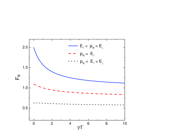
Figure 2: (Color online) Electron Fano factor $F_{e}$ as a function of relaxation rate $\gamma$ characterizing couplings to the outside environment in the absence of any driving field ($\Omega=0$). The Fano factor is found to decrease with the relaxation rate. Parameters: $\Delta_{z}=50~{}\mu$ev, $E_{\uparrow}=200~{}\mu$ev, $U=1$ mev, $\Gamma_{L}=\Gamma_{R}=\Gamma=5~{}\mu$ev, and $k_{B}T=1~{}\mu$ev.

In the regime $E_{\downarrow}>\mu_{R}>E_{\uparrow}$ ($\chi_{1}\approx 1$), the spin-up level is occupied most of the time since it is well below the chemical potentials of the two leads. Its occupation blocks further transport through others levels of the QD. This mechanism is termed as dynamic channel blockade, and it leads to enhanced shot noise [17, 11]. Once this spin-up electron tunnels out to the right lead due to thermal fluctuations, subsequent electron with either spin up or spin down tunnels into the QD. For a spin-up electron, we are back to the previous situation and just one electron is transported in this cycle. In contrast, for a spin-down electron, it can quickly tunnel to the right lead, or an additional spin-up electron enters the QD. A super-Poissonian shot noise due to the dynamic channel blockade results and the Fano factor is given by

$$F_{e}=1+\frac{6\Gamma_{L}\Gamma_{R}(\Gamma_{L}+\Gamma_{R})}{\Lambda_{1}},$$ (14)

where

$$\Lambda_{1}=\gamma(\Gamma_{L}+2\Gamma_{R})(2\Gamma_{L}+\Gamma_{R})+2(\Gamma_{L}+\Gamma_{R})(\Gamma_{L}^{2}+\Gamma_{L}\Gamma_{R}+\Gamma_{R}^{2}).$$ (15)

In Figure 2, the Fano factor is plotted as a function of the relaxation rate $\gamma$. It can be seen that the Fano factor decreases with the relaxation rate $\gamma$ in this regime. This is because the relaxation process increases the occupation of the spin-up state, which blocks further tunneling event and makes the current noise Poissonian.

In the large bias limit, i.e., $E_{\downarrow}>E_{\uparrow}>\mu_{R}$ ($\chi_{1}\approx 0$), tunneling for both spin orientations are allowed. The dynamic channel blockade is suppressed since the spin-up electron can now quickly tunnel into the right lead. Then, the current noise becomes sub-Poissonian with a negative correlation between electron transport events[30, 14]. We have

$$F_{e}=1-\frac{2\Gamma_{L}\Gamma_{R}\times\Lambda_{2}}{[2\gamma(\Gamma_{L}+\Gamma_{R})^{2}+\gamma\Gamma_{L}\Gamma_{R}+2(\Gamma_{L}+\Gamma_{R})^{3}]^{2}},$$ (16)

where

$$\Lambda_{2}\!=\!6\Gamma_{R}(\Gamma_{L}+\Gamma_{R})^{3}+2\gamma^{2}(\Gamma_{L}+2\Gamma_{R})^{2}+\gamma[\Gamma_{L}^{2}(2\Gamma_{L}+13\Gamma_{R})+\Gamma_{R}^{2}(23\Gamma_{L}+14\Gamma_{R})].$$ (17)

Our results explained here are different from those for a two-level-system case considered in Ref. [29], where the current noise is independent of the coupling to outside environment in the large bias regime. The transport mechanisms involving either of the two orbital levels discussed there are the same. As a result, the relaxation effect will not affect the current noise. For our system, the electron transport process depends on the precise state in the QD involved. With an initial spin-up electron, it will tunnel to the right lead. Starting from a spin-down state, it may tunnel to the right lead or an additional electron enters the QD to form a singlet. Even though the environment-induced relaxation have no direct effect on the singlet state, the noise shows a dependence on the relaxation effect [see Eq. (16)]. From Fig. 2, however, one notes that the effect of the relaxation does not alter the super- or sub-Poissonian characteristics of the shot noise in both regimes discussed above.

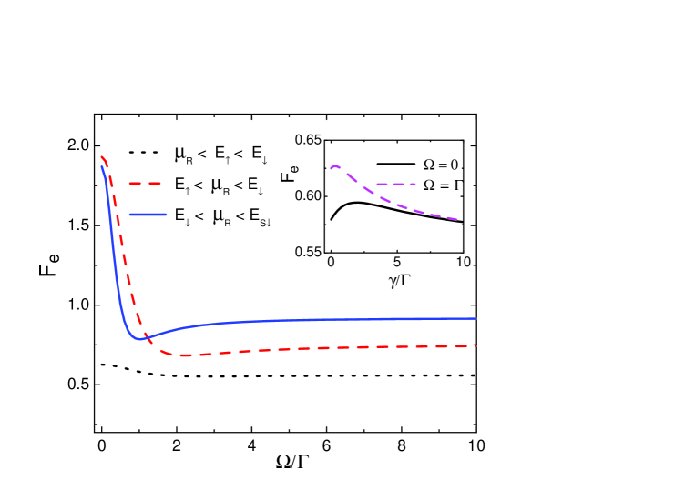
Figure 3: (Color online) Electron Fano factor $F_{e}$ as a function of the driving field strength $\Omega$ for $\gamma=0.1\Gamma$. At small driving field, super-Poissonian shot noise is obtained due to the interacting localized states in the regime $E_{\downarrow}<\mu_{R}<E_{S\downarrow}$. It is on the other hand due to dynamic channel blockade in the intermediate regime $E_{\uparrow}<\mu_{R}<E_{\downarrow}$. These two mechanisms are gradually suppressed by increasing the driving field intensity. At large $\Omega$, the noise becomes sub-Poissonian. Inset: the effect of driving field on electron noise in the large bias regime $\mu_{R}<E_{\uparrow}<E_{\downarrow}$. At small relaxation rate, the shot noise is different because of the effect of the driving field. At increasing relaxation rate, most tunneling events involve the spin-up state and the shot noise tends to be the same in two cases.

4.2 Noise properties with an ESR driving field

In this subsection, we discuss the effects of an ESR driving field on the current shot noise. The ESR driving field that induces spin flips between two opposite spin states will affect the transport through the QD differently in the three regimes considered above.

For $E_{S\downarrow}>\mu_{R}>E_{\downarrow}$, we have $\chi_{3}\approx 0$, and $\chi_{2}\approx\chi_{1}\approx 1$. The physical mechanism in this regime is similar to that for two interacting localized states discussed in Ref. [7], in which two impurity levels $M$ and $R$ were considered. When the transition rate through the lower impurity level $M$ is much smaller than that through the upper impurity level $R$, contribution of $M$ to the current is negligible. Due to Coulomb interaction between these two states, transport through $R$ is strongly modulated by the occupancy at $M$. As a result, the current jumps randomly between zero and a non-zero value. This modulation leads to an enhanced current shot noise [7].

Similarly, in our case, the main contribution to the current is from the transport via the singlet state. Another point we need to emphasize is that the system can only arrive at the singlet state starting from the spin-down state. Hence, current jumps randomly between zero and a non-zero value, e.g., $I_{0}$. The Fano factor is given by

$$F_{e}=1+\frac{2\Gamma_{L}\Gamma_{R}\times[\Theta_{1}(\gamma+\Gamma_{L})^{2}-\Theta_{2}\Omega^{2}]}{[\Theta_{1}(\Gamma_{L}+\gamma)+\Omega^{2}(3\Gamma_{L}+4\Gamma_{R})]^{2}},$$

(18)

where

$$\Theta_{1} = \Gamma_{L}(\Gamma_{L}+\Gamma_{R})+\gamma(\Gamma_{L}+2\Gamma_{R})$$

$$\Theta_{2} = 2(\Omega^{2}+\gamma^{2})+\gamma(7\Gamma_{L}+8\Gamma_{R})+\Gamma_{L}(5\Gamma_{L}+4\Gamma_{R}).$$ (19)

From Eq. (18), one notes that the current noise is super-Poissonian at a small driving field strength (see Fig. 3). With increasing field strength, however, the modulation of the current from the spin-up state will be suppressed by quick Rabi oscillations between the two spin states. As a result, the current noise changes from super-Poissoian to sub-Poissonian, as shown in Fig. 3.

When the right-lead chemical potential $\mu_{R}$ is tuned to the intermediate regime, $E_{\downarrow}>\mu_{R}>E_{\uparrow}$, with $\chi_{1}\approx 1$, and $\chi_{3}\approx\chi_{2}\approx 0$, the dynamic channel blockade will induce a super-Poissonian shot noise similar to the non-driven case in explained subsection 4.1. Furthermore, if the spin flips generated by the driving field are very frequent, the dynamic channel blockade will be suppressed. We then get

$$F_{e}\!=\!1+\frac{2\Gamma_{L}\Gamma_{R}}{\Xi_{1}^{2}}\{\Xi_{1}[3(\Gamma_{L}+\Gamma_{R}+\gamma)(\Gamma_{L}+\Gamma_{R})+4\Omega^{2}]-6\Omega^{2}\Xi_{2}(\Gamma_{L}+\Gamma_{R})\},$$ (20)

where

$$\Xi_{1}=2(\Gamma_{L}^{2}+\Gamma_{L}\Gamma_{R}+\Gamma_{R}^{2}+\gamma^{2}+3\Omega^{2})(\Gamma_{L}+\Gamma_{R})^{2}$$

$$+\gamma^{2}\Gamma_{L}\Gamma_{R}+\gamma(\Gamma_{L}+\Gamma_{R})(4\Gamma_{L}^{2}+7\Gamma_{L}\Gamma_{R}+4\Gamma_{R}^{2})$$

$$\Xi_{2}=(9\Gamma_{L}^{2}+13\Gamma_{L}\Gamma_{R}+9\Gamma_{R}^{2}+3\gamma^{2}+7\Omega^{2})(\Gamma_{L}+\Gamma_{R})+\gamma(12\Gamma_{L}^{2}+25\Gamma_{L}\Gamma_{R}+12\Gamma_{R}^{2}).$$ (21)

From Fig. 3, one can see that the Fano factor decreases gradually with increasing driving field strength. This indicates that the current shot noise changes from super-Poissoian to sub-Poissonian.

In the large bias regime, $E_{\downarrow}>E_{\uparrow}>\mu_{R}$, the current shot noise is always sub-Poissonian, as shown in Fig. 3. The expression for the Fano factor is too lengthy and is not shown here. Due to the interplay with the singlet state, our results are distinct from those without a driving field at a small relaxation rate. When the spin flips generated by the driving field is not able to compete with a large relaxation rate, however, the noise tends to be the same in the two cases, as shown in the inset of Fig. 3.

5 Conclusion

In conclusion, we have investigated current noise in a single QD under the influence of both external magnetic fields and the outside environment. When the dot is initially been occupied by an electron, the Zeeman splitting causes a spin-dependent energy cost for adding an additional electron, i.e., $E_{S\uparrow}\neq E_{S\downarrow}$. If the left-lead chemical potential $\mu_{L}$ lies within $E_{S\downarrow}$ and $E_{S\uparrow}$, the Coulomb blockade will be partially lifted. In this setup, the transport mechanisms for spin-up and spin-down electrons are different [31]. In previous studies [30], only a sub-Poissonian shot noise was found when the Coulomb blockade was completely lifted by applying a large bias voltage, i.e., $\mu_{L}>E_{S\uparrow(\downarrow)}$. However, in the full Coulomb blockade regime, a super-Poissonian shot noise was obtained in a QD containing two orbital levels due to dynamic channel blockade [29]. In the more general case considered here, we find a super-Poissonian electron shot noise induced by the effects of both interacting localized states and dynamic channel blockade via tuning the chemical potential of the right lead $\mu_{R}$. Moreover, we show that these mechanisms are suppressed by Rabi oscillations between the two spin states (generated by an ESR driving field). As a result, the current shot noise will change to sub-Poissonian at a large Rabi frequency.

References

References

- [1] Blanter Y M and Büttiker M 2000 Phys. Rep 336 1
- [2] Nazarov Yu V 2003 Quantum Noise in Mesoscopic Physics (Kluwer, Dordrecht)
- [3] Levitov L S and Lesovik G B 1993 JETP Lett. 58 230 ; Levitov L S, Lee H W and Lesovik G B 1996 J. Math. Phys. 37 4845
- [4] Khlus V A 1987 Sov. Phys. JETP 66 1243
- [5] Korotkov A N 1994 Phys. Rev. B. 49 10381
- [6] Lesovik G B 1989 JETP Lett. 49 592; Büttiker M 1990 Phys. Rev. Lett. 65 2901
- [7] Safonov S S, Savchenko A K, Bagrets D A, Jouravlev O N, Nazarov Y V, Linfield E H and Ritchie D A 2003 Phys. Rev. Lett. 91 136801
- [8] Kiesslich G, Wacker A and Schöll E 2003 Phys. Rev. B. 68 125320
- [9] Hershfield S, Davies J H, Hyldgaard P, Stanton C J and Wilkins J W 1993 Phys. Rev. B. 47 1967; Hanke U, Galperin Yu M, Chao K A and Zou N 1993 Phys. Rev. B. 48 17209
- [10] Chen L Y and Ting C S 1992 Phys. Rev. B. 46 4714
- [11] Belzig W 2005 Phys. Rev. B. 71 161301 (R)
- [12] Bulka B R, Martinek J, Michalek G and Barnas J 1999 Phys. Rev. B 60 12246; Bulka B R 2000 Phys. Rev. B. 62 1186
- [13] Gorelik L Y, Kulinich S I, Shekhter R I, Jonson M and Vinokur V M 2007 App. Phys. Lett. 90 192105
- [14] Djuric I, Dong B and Cui H L 2005 App. Phys. Lett. 87 032105
- [15] Elattri B and Gurvitz S A 2002 Phys. Lett. A. 292 289
- [16] Bagrets D A and Nazarov Yu V 2003 Phys. Rev. B. 67 085316
- [17] Cottet A, Belzig W and Bruder C 2004 Phys. Rev. Lett. 92 206801; Cottet A, Belzig W and Bruder C 2004 Phys. Rev. B. 70 115315
- [18] Sukhorukov E V, Burkard G and Loss D 2001 Phys. Rev. B. 63 125315
- [19] Thielmann A, Hettler M H, König J and Schön G 2005 Phys. Rev. Lett. 95 146806
- [20] Braun M, König J and Martinek J 2006 Phys. Rev. B. 74 075328
- [21] Weymann I and Barnaś J 2008 Phys. Rev. B. 77, 075305; Weymann I and Barnaś J 2007 J. Phys.: Condens. Matter. 19 096208
- [22] Chen Y and Webb R A 2006 Phys. Rev. B. 73 035424
- [23] Barthold P, Hohls F, Maire N, Pierz K and Haug R J 2006 Phys. Rev. Lett. 96 246804
- [24] Gustavsson S, Leturcq R, Simovi B, Schleser R, Studerus P, Ihn T, Ensslin K, Driscoll D C and Gossard A C 2006 Phys. Rev. B. 74 195305
- [25] Zhang Y, DiCarlo L, McClure D T, Yamamoto M, Tarucha S, Marcus C M, Hanson M P and Gossard A C 2007 Phys. Rev. Lett. 99 036603
- [26] Zarchin O, Chung Y C, Heiblum M, Rohrlich D and Umansky V 2007 Phys. Rev. Lett. 98 066801
- [27] Chen Y and Webb R A 2006 Phys. Rev. Lett. 97 066604
- [28] McClure D T, DiCarlo L, Zhang Y, Engel H A, Marcus C M, Hanson M P and Gossard A C 2007 Phys. Rev. Lett. 98 056801
- [29] Sánchez R, Platero G and Brandes T 2007 Phys. Rev. Lett. 98 146805
- [30] Djuric I, Dong B and Cui H L 2006 J. Appl. Phys. 99 063710
- [31] Engel H A and Loss D 2001 Phys. Rev. Lett. 86 4648
- [32] Sánchez R, Cota E, Aguado R, and Platero G 2006 Phys. Rev. B 74 035326
- [33] Johnson A C, Petta J R, Taylor J M, Yacoby A, Lukin M D, Marcus C M, Hanson M P and Gossard A C 2005 Nature 435 925
- [34] Plenio M B and Knight P L 1998 Rev. Mod. Phys. 70 101; Gurvitz S A and Prager Ya S 1996 Phys. Rev. B. 53 15932
- [35] Blum K 1996 Density Matrix Theory and Applications (Plenum, New York), Chap. 8
- [36] Martin I, Mozyrsky D and Jiang H W 2003 Phys. Rev. Lett. 90 018301
- [37] Lenstra D 1982 Phys. Rev. A. 26 3369
- [38] Dong B, Cui H L and Lei X L 2005 Phys. Rev. Lett. 94 066601