Exact relativistic tritium $\beta$-decay endpoint spectrum in a hadron model

Abstract

We present the relativistic calculation of the $\beta$-decay of tritium in a hadron model. The elementary particle treatment (EPT) of the transition ${}^{3}H\rightarrow^{3}He+e^{-}+\overline{\nu}_{e}$ is performed in analogy with the description of the $\beta$-decay of neutron. The effects of higher order terms of hadron current and nuclear recoil are taken into account in this formalism. The relativistic Kurie function is derived and presented in a simple form suitable for the determination of neutrino masses from the shape of the endpoint spectrum. A connection with the commonly used Kurie function is established.

I Introduction

Neutrinos are one of the most intriguing and fascinating fundamental particles, which make up the Universe. However, they are also one of the least understood particles. Studies of neutrinos have played a crucial role in the understanding of elementary particle laws and their interactions.

Three types of light neutrinos are known. The recent observation of neutrino oscillations SK ; SNO ; Kamland ; K2K ; Minos has now beyond doubt established the non-zero masses of neutrinos, the flavor change and neutrino mixing. It has opened a new excited era in neutrino physics and represents a big step forward in our knowledge of neutrino properties and serves as solution of many problems in cosmology, elementary particle physics, and astrophysics.

While neutrino oscillation experiments are sensitive only to differences of squared neutrino masses, the neutrino mass measurements with tritium ($Q_{\beta}(^{3}H)=18.6~{}keV$) and rhenium ($Q_{\beta}(^{187}Re)=2.47~{}keV$) $\beta$-decays yield direct information on the absolute neutrino mass scale. The idea underlying the measurement of neutrino mass is actually fairly obvious. A long time ago, it was already pointed out by E. Fermi fermi that the shape of the electron spectrum in nuclear $\beta$-decay, near the kinematical end point, is sensitive to the neutrino mass.

Attempts to evaluate the rest mass of the neutrino experimentally were already being undertaken long ago. In 1940 one of the first kinematical measurements of neutrino mass was performed by Hanna and Pontecorvo hanna with a proportional chamber filled with tritium. A limit of $\sim~{}1~{}keV$ on the neutrino mass was obtained, which was determined by the resolution of the detector. The Mainz mainz and Troitsk troitsk tritium $\beta$-decay experiments using the magnetic adiabatic collimation technique, place the present upper limit on the mass of the electron neutrino of $2.3~{}eV$ and $2.2~{}eV$, respectively. The best published calorimetric limit to the electron neutrino mass obtained from the $\beta$-spectrum of ${}^{187}Re$ is $15~{}eV$ mibeta . We note that the bounds on neutrino mass imposed by the shape of the spectrum are independent of whether neutrino is a Majorana or a Dirac particle.

A next-generation tritium $\beta$-decay experiment is the KArlsruhe TRItium Neutrino experiment (KATRIN) katrin ; drexlin ; wein , which is presently in construction phase (It is planned to take data starting 2010). This experiment is projected for measurement of the neutrino mass with a sensitivity of 200 meV, which will have important implications for the theory of neutrino masses. If the result will be positive, it will imply a degenerate spectrum of neutrino masses. On the other hand, a negative result will be a very useful constraint. There is also a chance that the planned MARE experiment mare based on arrays of rhenium low temperature microcalorimeters will be able to achieve sensitivity lower than 0.2 eV in future. The MARE approach would have totally different systematics with respect to the KATRIN.

In view of an enormous experimental progress in the field there is a request for a highly accurate theoretical description of the electron energy spectrum in the determination of the neutrino masses from the shape of the endpoint spectrum. The subject of interest has been molecular effects in tritium beta decay Doss , radiative corrections meissner , Lorentz invariance violations lorentz , interactions beyond the standard model goldman , relativistic form for the $\beta$-decay endpoint spectrum repko ; masood etc.

The aim of this paper is to derive the relativistic form for the $\beta$-endpoint spectrum in a hadron model. We shall take advantage of the fact that the nuclei ${}^{3}H$ and ${}^{3}He$ are, respectively, the nuclear analogs of the neutron and the proton, i.e., they form an isospin SU(2) doublet. A correspondence to the commonly used formulae will be established. We note that the considered approach is known also as Elementary Particle Treatment (EPT) of weak processes, which was developed by Kim and Primakoff kim .

II The nuclear physics description of tritium $\beta$-decay

By neglecting neutrino mixing for simplicity and taking into account only left-handed weak interaction, the electron energy spectrum for tritium $\beta$-decay is

$$N(E_{e}) = \frac{d\Gamma}{dE_{e}}$$ (1)

$$= \frac{G^{2}_{F}V^{2}_{ud}}{2\pi^{3}}|M.E.|^{2}F(Z,E_{e})p_{e}E_{e}$$

$$\times\left(E_{0}-E_{e}\right)\sqrt{(E_{0}-E_{e})^{2}-m^{2}_{\nu}},$$

where $G_{F}$ is the Fermi constant and $V_{ud}$ is the element of the Cabbibo-Kobayashi-Maskawa (CKM) matrix. $p_{e}$, $E_{e}$ and $E_{0}$ are the momentum, energy, and maximal endpoint energy (in the case of zero neutrino mass) of the electron, respectively. $F(Z,E)$ denotes the relativistic Coulomb factor.

The transition is superallowed, a mix of Fermi and Gamow-Teller transitions. The absolute square of the nuclear matrix element is given by

$$|M.E.|^{2}=f^{2}_{V}|M_{F}|^{2}+f^{2}_{A}|M_{GT}|^{2},$$ (2)

where the Fermi and Gamow-Teller matrix elements take the form

$$M_{F} = <^{3}He|\sum^{3}_{k=1}\tau^{+}_{k}|^{3}H>,$$ (3)

$${\vec{M}}_{GT} = <^{3}He|\sum^{3}_{k=1}\tau^{+}_{k}\vec{\sigma}_{k}|^{3}H>.$$ (4)

$f_{V}$ and $f_{A}$ are the vector and the axial-vector coupling constants of the nucleon, respectively. We note that the derivation of the differential decay rate in (1) involves non-relativistic approximations and that only the $s_{1/2}$ states of outgoing leptons are taken into account.

The Fermi matrix element can be evaluated by assuming the exact isospin symmetry as well as the fact that ${}^{3}H$ and ${}^{3}He$ form an isospin doublet $(T=1/2)$ (the projection $T_{z}=1/2$ is assigned to the ${}^{3}He$ and $T_{z}=-1/2$ to the ${}^{3}H$) with the result $M_{F}=1$.

The absolute square of the Gamow-Teller matrix element can be deduced from the Ikeda sum rule by taking into account that the Gamow-Teller operator has no radial dependence and thus can not scatter into higher shells. In ${}^{3}He$ the 1s neutron level is already occupied by two neutrons and therefore in the transition $p$ to $n$ the neutron would need to be scattered into a higher orbit (e. g., 2s) in the continuum, which is forbidden for the Gamow-Teller operator. Thus only ${}^{3}H\rightarrow^{3}He$ but not ${}^{3}H\rightarrow 3n$ can contribute to the Ikeda sum rule. In addition, there are no excited states of ${}^{3}He$. As a consequence $|M_{GT}|^{2}=3$. This result is in a good agreement with the recommended value $|M_{GT}|=\sqrt{3}(0.962\pm 0.002)$ obtained in nuclear structure calculation brown .

The conserved vector current (CVC) hypothesis proposed by Feynman and Gell-Mann suggests that the vector coupling constant $f_{V}$ is not renormalized in the nuclear medium, i.e., $f_{V}=1.0$. The accurately measured $\beta$-decay lifetime of tritium ($T_{1/2}(^{3}H)=12.32\pm 0.03~{}years$) budick ; hft is used to adjust the value of axial-vector coupling constant $f_{A}$ via the calculation of the theoretical half-life

$$\left(T_{1/2}\right)^{-1/2}=\frac{\Gamma}{\ln{2}}=\int_{m_{e}}^{E_{0}-m_{\nu}}N(E_{e})dE_{e}.$$ (5)

In the computation of the integral over the electron energy $E_{e}$ we adopted the relativistic Coulombic factor $F(Z,E)$ doi , which take into account the finite size of the nucleus. For $|M_{GT}|^{2}=3$ we found $|f_{A}|=1.247$. The very good agreement between this result and the bare nucleon value $|f_{A}/f_{V}|=1.2695\pm 0.0029$ PDG suggests that the axial-vector coupling constant is only weakly quenched in the tritium.

The dependence of spectrum shape on the mass of neutrino $m_{\nu}$ in (1) follows from the phase volume factors only. The traditional way to look at the $\beta$-spectrum data is to make a Kurie plot, where

$$K(E_{e}) \equiv \sqrt{\frac{N(E_{e})}{F(Z,E_{e})p_{e}E_{e}}}$$ (6)

$$= \frac{G_{F}V_{ud}}{\sqrt{2\pi^{3}}}|M.E|$$

$$\times\left(E_{0}-E_{e}\right)\sqrt[4]{1-\left(\frac{m_{\nu}}{(E_{0}-E_{e})}\right)^{2}}.$$

For zero mass neutrino, if $K(E_{e})$ is plotted against $E_{e}$, the result is a straight line that crosses the $E_{e}$ axis at $E_{e}=E_{0}$. For $m_{\nu}\neq 0$ the endpoint shifts to $E^{max}=E_{0}-m_{\nu}$ and the rate near the endpoint is depressed, namely the Kurie plot has a kink at the endpoint. This distortion will be washed out at the experiment unless the energy resolution is comparable to $m_{\nu}$.

There are open questions related to the presented conventional approach for kinematical study of the $\beta$-decay endpoint of ${}^{3}H$. In particular, it is not known what the consequences of the considered non-relativistic approximations are. Further, the effect of the nuclear recoil is not taken into account. It is also worth mentioning that the relativistic expression for the maximal electron energy

$$E^{max}_{e}=\frac{1}{2M_{f}}\left[M^{2}_{i}+m^{2}_{e}-(M_{f}+m_{\nu})^{2}\right],$$ (7)

gives a value about $3.4~{}eV$ lower than the considered approximation $E^{max}_{e}\simeq M_{i}-M_{f}-m_{\nu}$ masood ($M_{i}$, $M_{f}$ and $m_{e}$ are masses of the tritium atom, ${}^{3}He^{+}$ and the electron, respectively). In view of the planned sensitivity of $\sim 0.2~{}eV$ of the KATRIN experiment, there is a request for a consistent relativistic description of the $\beta$-decay of tritium masood .

III Relativistic $\beta$-decay kinematics in hadron model

We shall study the $\beta$-decay of tritium,

$${}^{3}H~{}\rightarrow~{}^{3}He~{}+~{}e^{-}~{}+{\overline{\nu}}_{e},$$ (8)

in an analogy with the $\beta$-decay of a free neutron,

$$n~{}\rightarrow~{}p~{}+~{}e^{-}~{}+{\overline{\nu}}_{e},$$ (9)

as the spin-isospin characteristics of ${}^{3}H$ (${}^{3}He$) nucleus and neutron (proton) are the same. The kinematics of the two processes above differ mostly due to different Q-values and the Coulomb corrections.

The invariant $\beta$-decay amplitude is given by

$${M} = \frac{G_{F}V_{ud}}{\sqrt{2}}~{}\overline{u}(P_{e})\gamma_{\alpha}(1-\gamma_{5})v(P_{\nu})$$

$$\times\overline{u}(P_{f})\left[G_{V}(q^{2})\gamma^{\alpha}+i\frac{G_{M}(q^{2})}{2M_{i}}\sigma^{\alpha\beta}q_{\beta}\right.$$

$$\left.~{}~{}~{}~{}~{}~{}~{}~{}~{}-G_{A}(q^{2})\gamma^{\alpha}\gamma_{5}-G_{P}(q^{2})q^{\alpha}\gamma_{5}\right]u(P_{i}).$$

Here, $q_{\alpha}=(P_{f}-P_{i})_{\alpha}=(P_{e}+P_{\nu})_{\alpha}$ is the momentum transferred to the hadron vertex. $P_{i}=(M_{i},0)$, $P_{f}=(M_{f},{\mathbf{p_{f}}})$, $P_{e}=(m_{e},{\mathbf{p_{e}}})$ and $P_{\nu}=(m_{\nu},{\mathbf{p_{\nu}}})$ are four momenta of the ${}^{3}H$, ${}^{3}He$, electron and antineutrino in the laboratory frame, respectively.

The form factors $G_{V}(q^{2})$, $G_{M}(q^{2})$, $G_{A}(q^{2})$, $G_{P}(q^{2})$ are real functions of the squared momentum $q^{2}$. They are parameterized as follows:

$$G_{V}(q^{2}) = \frac{g_{V}}{\left(1-\frac{q^{2}}{M^{2}_{V}}\right)^{2}},~{}~{}~{}~{}G_{M}(q^{2})=\frac{g_{M}}{\left(1-\frac{q^{2}}{M^{2}_{V}}\right)^{2}},$$

$$G_{A}(q^{2}) = \frac{g_{A}}{\left(1-\frac{q^{2}}{M^{2}_{A}}\right)^{2}}.$$ (11)

The two form-factor cut-offs $M_{V}$ and $M_{A}$ are in general different and their values are expected to be of the order of $1~{}GeV$ like it is in the case of nucleon form-factors. As it will be discussed later the $q^{2}$-dependence of these form-factors is not crucial for tritium $\beta$-decay.

The conserved vector current hypothesis (CVC) implies $g_{V}=1.0$. $g_{M}=-6.106$ is calculated from the values of magnetic moments of ${}^{3}H$ and ${}^{3}He$ using the CVC hypothesis as well stone . The axial coupling constant $g_{A}$ can be determined from the measured half-life of ${}^{3}H$. The induced pseudoscalar coupling is given by the partially conserved axial-vector current hypothesis (PCAC)

$$g_{P}(q^{2})={2M_{i}g_{A}(q^{2})}/({m^{2}_{\pi}-{q}^{2}}).$$ (12)

$m_{\pi}$ is the mass of pion.

For the spin-summed, Lorentz-invariant squared amplitude we get

$$\frac{1}{2}\sum_{spins}|{M}|^{2}=16(G_{F}V_{ud})^{2}~{}~{}~{}~{}~{}~{}~{}~{}~{}~{}~{}~{}$$

$$\times\left[G^{2}_{V}{\cal P}_{VV}+G_{A}G_{V}{\cal P}_{AV}+G^{2}_{A}{\cal P}_{AA}+~{}~{}~{}~{}~{}\right.$$

$$+G_{A}G_{P}{\cal P}_{AP}+G^{2}_{P}{\cal P}_{PP}~{}~{}~{}~{}~{}~{}~{}~{}~{}~{}~{}~{}~{}$$

$$\left.+G_{V}G_{M}\frac{{\cal P}_{VM}}{2M_{i}}+G_{A}G_{M}\frac{{\cal P}_{AM}}{2M_{i}}+G_{M}^{2}\frac{{\cal P}_{MM}}{4M^{2}_{i}}\right]$$

(13)

with

$${\cal P}_{VV}=P_{ef}P_{\nu i}+P_{ei}P_{\nu f}-M_{i}M_{f}P_{e\nu},$$ (14)

$${\cal P}_{AA}=P_{ef}P_{\nu i}+P_{ei}P_{\nu f}+M_{i}M_{f}P_{e\nu},$$ (15)

$${\cal P}_{AV}=2\left(P_{ef}P_{\nu i}-P_{ei}P_{\nu f}\right),$$ (16)

$${\cal P}_{AP}=M_{f}(m^{2}_{e}P_{\nu i}+m^{2}_{\nu}P_{ei})-M_{i}(m^{2}_{e}P_{\nu f}+m^{2}_{\nu}P_{ef}),$$ (17)

$${\cal P}_{PP}~{}=~{}\frac{1}{2}(P_{if}-M_{i}M_{f})\left(P_{e\nu}(m^{2}_{e}+m^{2}_{\nu})+2m^{2}_{\nu}m^{2}_{e}\right),$$ (18)

$${\cal P}_{VM}=~{}~{}~{}~{}~{}~{}~{}~{}~{}~{}~{}~{}~{}~{}~{}~{}~{}~{}~{}~{}~{}~{}~{}~{}~{}~{}~{}~{}~{}~{}~{}~{}~{}~{}~{}~{}$$

$$~{}M_{i}\left[P_{e\nu}(P_{if}-M^{2}_{f})+P_{ef}(P_{\nu i}-2P_{\nu f})+P_{ei}P_{\nu f}\right]$$

$$+M_{f}\left[P_{e\nu}(P_{if}-M^{2}_{i})+P_{ei}(P_{\nu f}-2P_{\nu i})+P_{ef}P_{\nu i}\right],$$ (19)

$${\cal P}_{AM}=2(M_{i}+M_{f})(P_{ef}P_{\nu i}-P_{ei}P_{\nu f}),$$ (20)

$${\cal P}_{MM}~{}=~{}~{}~{}~{}~{}~{}~{}~{}~{}~{}~{}~{}~{}~{}~{}~{}~{}~{}~{}~{}~{}~{}~{}~{}~{}~{}~{}~{}~{}~{}~{}~{}~{}~{}$$

$$-\frac{1}{2}P_{if}\left(P_{e\nu}(m^{2}_{e}+m^{2}_{\nu})+2m^{2}_{e}m^{2}_{\nu}\right)-M_{i}M_{f}m^{2}_{e}m^{2}_{\nu}$$

$$+2P_{ei}P_{ef}(P_{e\nu}+m^{2}_{\nu})+2P_{\nu i}P_{\nu f}(P_{e\nu}+m^{2}_{e})~{}~{}~{}~{}~{}~{}~{}$$

$$-\frac{1}{2}M_{i}M_{f}P_{e\nu}\left(3m^{2}_{e}+3m^{2}_{\nu}+4P_{e\nu}\right).~{}~{}~{}~{}~{}~{}~{}~{}~{}~{}~{}~{}~{}$$ (21)

Here, $P_{kl}\equiv\left(P_{k}\cdot P_{l}\right)$ with $k,l=i,~{}f,~{}e$ and $\nu$ denotes the scalar product of two four-momenta.

By neglecting the contribution from higher order currents (terms proportional to $G_{M,P}$) we find

$$\frac{1}{2}\sum_{spins}|{M}|^{2}=16(G_{F}V_{ud})^{2}~{}~{}~{}~{}~{}~{}~{}~{}~{}~{}~{}~{}$$

$$\times\left[(G_{V}+G_{A})^{2}(P_{e}\cdot P_{f})(P_{\nu}\cdot P_{i})~{}~{}~{}~{}~{}~{}\right.$$

$$+(G_{V}-G_{A})^{2}(P_{e}\cdot P_{i})(P_{\nu}\cdot P_{f})~{}~{}~{}~{}~{}~{}$$

$$\left.(-G^{2}_{V}+G^{2}_{A})M_{i}M_{f}(P_{e}\cdot P_{\nu})\right].~{}~{}~{}~{}~{}~{}$$ (22)

The advantage of the presented formalism is that the squared Lorentz invariant amplitude is calculated exactly unlike in Ref. masood , where an assumption about its dominant constituent was considered. We note that for $G_{V}=G_{A}=1$ the squared amplitude is proportional to $(P_{e}\cdot P_{f})(P_{\nu}\cdot P_{i})$, i.e., the structure is similar as, e.g., in the case of the muon decay.

For the tritium $\beta$-decay at rest the differential decay rate is

$$d\Gamma = \frac{1}{2M_{i}}F(Z,E_{e})\left(\frac{1}{2}\sum_{spins}|{M}|^{2}\right)$$

$$\times\frac{(2\pi)^{4}}{(2\pi)^{9}}\delta^{(4)}(P_{i}-P_{f}-P_{e}-P_{\nu})\frac{d^{3}p_{e}}{2E_{e}}\frac{d^{3}p_{\nu}}{2E_{\nu}}\frac{d^{3}p_{f}}{2E_{f}}.$$

The factor $1/2$ in front of the squared amplitude stands for the average over the spin of the initial state.

The subject of interest is the energy distribution of the electron. Hence, the integration over antineutrino and final nucleus momenta have to be performed in (LABEL:eq:11). It requires calculation of the following integrals:

$${\cal K} = \int\frac{d^{3}p_{f}}{E_{f}}\frac{d^{3}p_{\nu}}{E_{\nu}}~{}\delta^{(4)}(Q-P_{f}-P_{\nu}),$$ (24)

$$({\cal L}_{\nu,f})^{\rho} = \int\frac{d^{3}p_{f}}{E_{f}}\frac{d^{3}p_{\nu}}{E_{\nu}}~{}\delta^{(4)}(Q-P_{f}-P_{\nu})(P_{\nu,f})^{\rho},$$ (25)

$$({\cal N}_{kl})^{\rho\sigma} = \int\frac{d^{3}p_{f}}{E_{f}}\frac{d^{3}p_{\nu}}{E_{\nu}}~{}\delta^{(4)}(Q-P_{f}-P_{\nu})(P_{k})^{\rho}(P_{l})^{\sigma}$$

with $Q=P_{i}-P_{e}$ and $k,l=\nu,f$. The details of integrations with results are given in the Appendix.

The differential decay rate is found to be of the form

$$\frac{d\Gamma}{dE_{e}} = \frac{1}{2\pi^{3}}(G_{F}V_{ud})^{2}F(Z,E_{e})p_{e}$$

$$\times\frac{M^{2}_{i}}{(m_{12})^{2}}\sqrt{y\left(y+2m_{\nu}\frac{M_{f}}{M_{i}}\right)}$$

$$\times\left[g^{2}_{V}{\cal R}_{VV}+g_{A}g_{V}{\cal R}_{AV}+g^{2}_{A}{\cal R}_{AA}+\right.$$

$$~{}~{}~{}~{}~{}~{}~{}+g_{A}g_{P}{\cal R}_{AP}+g^{2}_{P}{\cal R}_{PP}$$

$$~{}~{}\left.+g_{V}g_{M}{\cal R}_{VM}+g_{A}g_{M}{\cal R}_{AM}+g_{M}^{2}{\cal R}_{MM}\right],$$

where $(m_{12})^{2}=M_{i}^{2}+m_{e}^{2}-2M_{i}E_{e}$ and $y=E^{max}_{e}-E_{e}$. In the calculation we neglected $q^{2}$ dependence of the form-factors as for the $\beta$-decay of ${}^{3}H$ the value of $q^{2}$ is rather small. Their consideration would lead only to small correction factors, which are not sensitive to neutrino mass. We find not usefull to present here the explicit form of all ${\cal R}_{I}$ ($I=VV,~{}VA,~{}AA,~{}AP,~{}PP,~{}VM,~{}AM,~{}MM$) factors. Instead of that we conclude about their structure and importance.

Our analysis showed that each term of ${\cal R}_{I}$ is proportional to $(y+m_{\nu}({M_{f}+m_{\nu}})/{M_{i}})$ or $(y+m_{\nu}{M_{f}}/{M_{i}})$. So, a common $(y+m_{\nu}{M_{f}}/{M_{i}})$ can be put in front of the bracket in (LABEL:eq:13) by neglecting a small term $m_{\nu}/M_{i}$. The importance of different ${\cal R}_{I}$ contributions can be studied in the limit $M_{i}=M_{f}$, $E_{e}=m_{e}$ and by making Taylor expansion in in $m_{\nu}$, $m_{e}$ ($m_{\nu}\ll m_{e}\ll M_{i}$). The leading terms of different ${\cal R}_{I}$ (without the common factor) are as follows:

$$VV:~{}m_{e}M_{i},~{}~{}~{}AA:~{}3m_{e}M_{i},~{}~{}~{}AV:~{}2m^{2}_{e},~{}~{}~{}$$

$$VM:~{}\frac{1}{2}\frac{m^{3}_{e}}{M_{i}},~{}~{}~{}MM:~{}\frac{3}{16}\frac{m^{5}_{e}}{M^{3}_{i}},~{}~{}~{}AM:~{}2m^{2}_{e},~{}~{}$$

$$AP:~{}2m_{e}M_{i}\frac{m^{2}_{e}}{m^{2}_{\pi}},~{}~{}PP:~{}\frac{1}{2}m_{e}M_{i}\frac{m^{4}_{e}}{M^{2}_{i}m_{\pi}^{2}}.~{}~{}~{}~{}~{}~{}~{}$$

(28)

From their comparison we conclude that the contributions coming from higher order terms of hadron current to the decay rate of ${}^{3}H$ can be neglected.

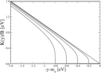
Figure 1: Endpoints of the relativistic Kurie plot [see Eqs. (31) and (32)] of the tritium beta decay for various values of the neutrino mass: $m_{\nu}=0,~{}0.2,~{}0.4,~{}0.6,$ and $0.8~{}eV$.

Then we have

$$\frac{d\Gamma}{dE_{e}} = \frac{1}{2\pi^{3}}(G_{F}V_{ud})^{2}F(Z,E_{e})p_{e}$$ (29)

$$\times\frac{M^{2}_{i}}{(m_{12})^{2}}\sqrt{y\left(y+2m_{\nu}\frac{M_{f}}{M_{i}}\right)}$$

$$\times\left[(g_{V}+g_{A})^{2}y\left(y+m_{\nu}\frac{M_{f}}{M_{i}}\right)\frac{M_{i}^{2}(E^{2}_{e}-m^{2}_{e})}{3(m_{12})^{4}}\right.$$

$$~{}~{}(g_{V}+g_{A})^{2}(y+m_{\nu}\frac{M_{f}+m_{\nu}}{M_{i}})\frac{(M_{i}E_{e}-m_{e}^{2})}{m_{12}^{2}}$$

$$~{}~{}~{}~{}~{}~{}~{}~{}~{}~{}~{}~{}\times(y+M_{f}\frac{M_{f}+m_{\nu}}{M_{i}})\frac{(M_{i}^{2}-M_{i}E_{e})}{m_{12}^{2}}$$

$$~{}-(g_{V}^{2}-g^{2}_{A})M_{f}\left(y+m_{\nu}\frac{(M_{f}+M_{\nu})}{M_{i}}\right)$$

$$~{}~{}~{}~{}~{}~{}~{}~{}~{}~{}~{}~{}~{}~{}~{}~{}~{}\times\frac{(M_{i}E_{e}-m^{2}_{e})}{(m_{12})^{2}}$$

$$~{}\left.+(g_{V}-g_{A})^{2}E_{e}\left(y+m_{\nu}\frac{M_{f}}{M_{i}}\right)\right].$$

The first term in the brackets in (29), which is quadratic in y, plays a subleading role. By keeping only the dominant contributions and by introducing a mass scale parameter $M$ instead of the $M_{i}$ and $M_{f}$, we get

$$\frac{d\Gamma}{dE_{e}} \simeq \frac{1}{2\pi^{3}}(G_{F}V_{ud})^{2}F(Z,E_{e})p_{e}E_{e}(g^{2}_{V}+3g^{2}_{A})$$ (30)

$$\times\sqrt{y\left(y+2m_{\nu}\right)}\left(y+m_{\nu}\right).$$

For the relativistic form of the Kurie function we can write

$$K(y)=B\left(\sqrt{y\left(y+2m_{\nu}\right)}\left(y+m_{\nu}\right)\right)^{1/2}$$ (31)

with

$$B=\frac{G_{F}V_{ud}}{\sqrt{2\pi^{3}}}\sqrt{g^{2}_{V}+3g^{2}_{A}}.$$ (32)

The unknown coupling constant $g_{A}$ of the hadron current is fixed to the half-life of ${{}^{3}H}$ budick ; hft with result $g_{A}=1.247$. This value coincides well with that of the axial-vector coupling of the nucleon (see previous section). We have $B=3.43\times 10^{-6}~{}GeV^{-2}$.

By comparing the Kurie function in (31) and (32) with the commonly used one (6) we find that they are equal if $y$ is replaced with $(E_{0}-E_{e}-m_{\nu})$ and $|M_{GT}|^{2}=3$ is assumed. This confirms what was generally expected, namely that the relativistic effects are small corrections to the results known in the traditional method due to a small $Q$-value of the $\beta$-decay of tritium. However, it was not clear yet whether the recoil of the nucleus, which value is $3.4$ eV for maximal electron energy, affects the endpoint spectra, if sub eV mass of neutrino is measured. Within the considered EPT of $\beta$-decay of tritium we find that there is no significant modification of the shape of the electron spectra close to the endpoint due to the nuclear recoil.

In Fig. 1 we show a relativistic Kurie plot for the $\beta$-decay of ${}^{3}H$ versus $y=E^{max}-E_{e}$ near the endpoint. Special attention is given to the effect of a small neutrino mass ($m_{\nu}=0.2,~{}0.4,~{}0.6$ and $0.8~{}eV$). We see that the Kurie plot is linear near the endpoint for zero neutrino mass ($m_{\nu}=0$). However, the linearity of the Kurie plot is lost if the neutrino has a non-zero mass. Deviation from a straight line depends on the magnitude of neutrino mass $m_{\nu}$. Though, there is no difference with the previously known dependences, it is worth to stress that in this case the relativistic form of the $\beta$-decay Kurie plot is used, which also takes the nuclear recoil ($\sim 3.4$ eV) into account.

IV Conclusion

The neutrino absolute mass scale, which is very important for particle physics as well as for cosmology and astrophysics, cannot be resolved by oscillation experiments. A way of the direct determination of the neutrino mass scale in laboratory experiment is the investigation of the kinematics of tritium $\beta$-decay.

The KATRIN experiment katrin ; drexlin ; wein , which is under construction, will be able to reach a sensitivity of neutrino mass in the sub-eV range. In connection with that there is a request for a highly accurate theoretical description of the electron energy spectrum.

In this paper we derived the relativistic form for the $\beta$-decay endpoint spectrum in the elementary particle treatment of weak interaction. The considered formalism follows from the analogy between ${}^{3}H$ (${}^{3}He$) and the neutron (proton) having the same spin-isospin properties. It allowed us unlike in Ref. masood to determine the squared $\beta$-decay amplitude more accurately. In addition, we found that the higher order terms of the hadron current can be neglected without affecting the dependence of the Kurie plot on the electron energy and the neutrino mass. By comparing the relativistic and previously used Kurie functions a good agreement between them was established.

We acknowledge the support of the EU ILIAS project under the contract RII3-CT-2004-506222, the Deutsche Forschungsgemeinschaft (436 SLK 17/298) and of the VEGA Grant agency of the Slovak Republic under the contract No. 1/0249/03.

Appendix A

Here we outline the calculation of integrals over neutrino and final nuclear momenta.

Integration of ${\cal K}$:
The integration is performed by choosing $Q=(Q_{0},\mathbf{0})$, i.e., the rest frame connected with the center of mass of antineutrino and final nucleus. We have

$${\cal K} = \int\int\frac{d^{3}p_{f}}{E_{f}}\frac{d^{3}p_{\nu}}{E_{\nu}}~{}\delta^{(4)}(Q-P_{f}-P_{\nu})$$

$$= \int\frac{1}{E_{\nu}}~{}\delta(Q_{0}-E_{f}-E_{\nu})~{}{p_{f}dE_{f}d\Omega_{f}}$$

with $E_{f}=(m_{\nu}^{2}-M^{2}_{f}+E_{f}^{2})^{1/2}$. By using $\delta(f(x))=\delta(x-x_{0})/{|f^{\prime}(x_{0})|}$ we find

$${\cal K}=2\pi\frac{\sqrt{[Q^{2}_{0}-(M_{f}+m_{\nu})^{2}][Q^{2}_{0}-(M_{f}-m_{\nu})^{2}]}}{Q^{2}_{0}}.$$

We replace $Q_{0}^{2}$ with $Q^{2}$ and write ${\cal K}$ in the Lorentz invariant form

$${\cal K} = 2\pi\frac{\sqrt{[Q^{2}-(M_{f}+m_{\nu})^{2}][Q^{2}-(M_{f}-m_{\nu})^{2}]}}{Q^{2}}$$ (35)

$$= 4\pi M_{i}\frac{\sqrt{y\left(y+2m_{\nu}\frac{M_{f}}{M_{i}}\right)}}{(m_{12})^{2}}.$$

Integration of $({\cal L}_{\nu})^{\rho}$:
The integral

$$({\cal L}_{\nu})^{\rho} = \int\frac{d^{3}p_{f}}{E_{f}}\frac{d^{3}p_{\nu}}{E_{\nu}}~{}\delta^{(4)}(Q-P_{f}-P_{\nu})(P_{\nu})^{\rho}$$

can be written as

$$({\cal L}_{\nu})^{\rho}=AQ^{\rho}.$$ (37)

Here, $A\equiv A(Q^{2})$ is a scalar function of $Q^{2}$. By multiplying $({\cal L}_{\nu})^{\rho}$ with $Q_{\rho}$ the constant $A(Q^{2})$ can be determined. Then we get

$$({\cal L}_{f})^{\rho}=\frac{(Q\cdot P_{f})}{Q^{2}}~{}{\cal K}~{}~{}Q^{\rho}.$$ (38)

Integration of $({\cal N}_{\nu f})^{\rho\sigma}$:
The integral

$$({\cal N}_{\nu f})^{\rho\sigma} = \int\frac{d^{3}p_{f}}{E_{f}}\frac{d^{3}p_{\nu}}{E_{\nu}}~{}\delta^{(4)}(Q-P_{f}-P_{\nu})(P_{\nu})^{\rho}(P_{f})^{\sigma}$$

is a second rank tensor

$$({\cal N}_{\nu f})^{\rho\sigma}=Cg^{\rho\sigma}+DQ^{\rho}Q^{\sigma},$$ (40)

where $C\equiv C(Q^{2})$ and $D\equiv D(Q^{2})$ are scalar functions of $Q^{2}$.

By multiplying $({\cal N}_{\nu f})^{\rho\sigma}$ with $g^{\mu\nu}$ and with $Q_{\rho}Q_{\sigma}$ a set of two equations is formed. By solving them we find

$$\frac{({\cal N}_{\nu f})^{\rho\sigma}}{\cal K} = \left(\left(P_{\nu}\cdot P_{f}\right)-\frac{\left(Q\cdot P_{\nu}\right)\left(Q\cdot P_{f}\right)}{Q^{2}}\right)~{}\frac{1}{3}g^{\rho\sigma}$$

$$-\left(\left(P_{\nu}\cdot P_{f}\right)-4\frac{\left(Q\cdot P_{\nu}\right)\left(Q\cdot P_{f}\right)}{Q^{2}}\right)\frac{Q^{\rho}Q^{\sigma}}{3Q^{2}}.$$

The remaining integrals $({\cal L}_{\nu})^{\rho}$, $({\cal N}_{\nu\nu})^{\rho\sigma}$, $({\cal N}_{ff})^{\rho\sigma}$ can be calculated following the scheme given above.

References

• (1) Super-Kamiokande Collaboration, S. Fukuda et al., Phys. Rev. Lett. 81, 1562 (1998); Y. Ashie et al., Phys. Rev. Lett. 93, 101801 (2004); Phys. Rev. Lett. 93, 101801 (2004); Phys. Rev. D 71, 112005 (2005).
• (2) SNO collaboration, Q.R. Ahmed et al., Phys. Rev. Lett. 87, 071301 (2001); Phys. Rev. Lett. 89, 011301 (2002); Phys. Rev. Lett. 89, 011302 (2002); B. Aharmim et al., Phys. Rev. C 72, 055502 (2005).
• (3) KamLAND collaboration, T.Araki et al., Phys. Rev. Lett. 94, 081801 (2004); Phys. Rev. Lett. 94, 081801 (2005).
• (4) K2K Collaboration, M.H. Alm et al., Phys. Rev. Lett. 90, 041801 (2003); E. Aliu et al., Phys. Rev. Lett. 94, 081802 (2005).
• (5) MINOS Collaboration, D.G. Michael et al., Phys. Rev. Lett. 97, 191801 (2006).
• (6) E. Fermi, Z. Phys. 88, 161 (1934).
• (7) G. Hanna and B. Pontecorvo, Phys. Rev. 75, 983 (1949).
• (8) Ch. Kraus et al., Eur. Phys. J. C 40, 447 (2005).
• (9) V.M. Lobashev, Nucl. Phys. A 719, 153 (2003).
• (10) M. Sisti et al., Nucl. Instrum. Meth. A 520, 125 (2004).
• (11) MARE Collaboration, E. Andreotti et al., Nucl. Instrum. Meth. A 572, 208 (2007); M. Sisti for MARE Collaboration, Nucl. Phys. B 168, 48 (2007).
• (12) KATRIN Collaboration, A. Osipowicz et al., hep-ex/0109033; L. Bornschein et al., Nucl. Phys. A 752, 14 (2005).
• (13) G. Drexlin for the KATRIN Collaboration, Nucl. Phys. Proc. Suppl. 145, 263 (2005).
• (14) C. Weinheimer, Nucl. Phys. Proc. Suppl. 168, 5 (2007).
• (15) N. Doss, J. Tennyson, A. Saenz, S. Jonsell, Phys. Rev. C 73, 025502 (2006).
• (16) S. Gardner, V. Bernard, and Ulf-G. Meißner, Phys. Lett. B 598, 188 (2004).
• (17) J.M. Carmona and J.L. CortΓ©s, Phys. Lett. B 494, 75 (2000).
• (18) G.J. Stephenson, Jr., T. Goldman, and B.H.J. McKellar, Phys. Rev. D 62, 093013.
• (19) C.E. Wu, W.W. Repko, Phys. Rev. C 27, 1754 (1983).
• (20) S.S. Masood, S. Nasri, J. Schechter, M.A. TΓ³rtola, J.W.F. Valle, and C. Weinheimer, Phys. Rev. C 76, 045501 (2007).
• (21) C.W. Kim and H. Primakoff, Phys. Rev. 139, B 1447 (1965); 140, B 566 (1965); C.W. Kim, Phys. Rev. 146, 691 (1966).
• (22) J.J. Simpson, Phys. Rev. C 35, 752 (1987).
• (23) B. Budick, J. Chen, and H. Lin, Phys. Rev. Lett. 67, 2630 (1991).
• (24) G.E. Brown and W. Weise, Phys. Rep. 22, 280 (1975).
• (25) Particle Data Group, W.M. Yao et al., J. Phys. G 33, 1 (2006).
• (26) M. Doi, T. Kotani and E. Takasugi, Prog. Theor. Phys. (Supp.) 83, 1 (1985).
• (27) N.J. Stone, Oxford University preprint, http://ie.lbl.gov/toi.html