Descents and nodal load in scale-free networks

Abstract

The load of a node in a network is the total traffic going through it when every node pair sustains a uniform bidirectional traffic between them on shortest paths. We show that nodal load can be expressed in terms of the more elementary notion of a node’s descents in breadth-first-search (BFS or shortest-path) trees, and study both the descent and nodal-load distributions in the case of scale-free networks. Our treatment is both semi-analytical (combining a generating-function formalism with simulation-derived BFS branching probabilities) and computational for the descent distribution; it is exclusively computational in the case of the load distribution. Our main result is that the load distribution, even though it can be disguised as a power-law through subtle (but inappropriate) binning of the raw data, is in fact a succession of sharply delineated probability peaks, each of which can be clearly interpreted as a function of the underlying BFS descents. This find is in stark contrast with previously held belief, based on which a power law of exponent $-2.2$ was conjectured to be valid regardless of the exponent of the power-law distribution of node degrees.

I Introduction

In a scale-free network, node connectivities (or degrees) are distributed according to a power law, that is, the probability that a randomly chosen node has degree $k$ is proportional to $k^{-\tau}$ for some $\tau>1$. Scale-free networks are therefore strictly diverse from networks of the classic Erdős-Rényi type Erdős and Rényi (1959), in which node degrees are Poisson-distributed. The importance of scale-free networks in various natural, social, and technological settings (the latter encompassing now ubiquitous structures such as the Internet and the WWW) has motivated considerable research along several fronts during the last decade. For the main results that have been attained the reader is referred to Boccaletti et al. (2006) and to the chapters in Bornholdt and Schuster (2003); Newman et al. (2006).

Most of these research efforts have been focused on either extracting a scale-free network structure out of data on some particular domain, or the creation of mechanisms of network evolution to function as generative models of such networks. As a consequence, it seems fair to state that so far the greatest thrust has been directed toward what may be called the “syntactic” aspects of scale-free networks, as opposed to their “semantic” (or “functional”) aspects, these being related to the higher processes, either natural or artificial, that depend on the underlying networks as a substrate. In the case of computer networks, for example, this issue is illustrated by the networks’ topological properties, on the one hand, and their utilization (for end-to-end communication protocols, data storage and retrieval, etc.), on the other.

Still in the context of computer networks, exceptions to the research trend just mentioned can be found in the works reported in Stauffer and Barbosa (2006a, b, 2007), all concerned with the efficient, global dissemination of information through the nodes of a network. The common thread that runs through all three of them is that degree-based local heuristics exist for forwarding information through the nodes of the network so that, globally, good statistical properties are achieved (such as expecting delivery to occur for most nodes, for example). However, when disseminating information globally is the goal, we find that designing heuristics based on node degrees, even though meritorious by their eminently local nature, is somewhat lacking in plausibility, since important performance-related notions, like locally available bandwidth and and node congestion, for example, remain inadequately accounted.

We see, then, that even as we move from the merely topological aspects of a network toward its higher-level, functional aspects, there remain entities that make up a node’s set of local characteristics (e.g., node congestion) which ultimately can be understood as originating higher up at more abstract levels (e.g., the protocols that steer information this way or that as it moves through the network). Clearly, understanding such entities seems to be one of the fundamental keys to better design decisions at the upper levels. And even though the setting of computer networks provides good examples here, note that very similar issues are present in other contexts, such as that of networks representing road or street maps and, in fact, any other network where end-to-end flows of some sort intersect one another.

In this paper we study the load of a node in a scale-free network. This property was originally introduced and analyzed in Goh et al. (2001) and gives, for the node in question, the total communication demand on that node when all node pairs sustain a uniform, bidirectional message traffic between them on shortest paths. Clearly, the load of a node is one of the aforementioned entities, bridging the various levels of abstraction at which the network may be analyzed. The study in Goh et al. (2001) is essentially based on simulations and ends with the conjecture that nodal load is distributed as a power law whose exponent is invariant with respect to $\tau$ in the range $(2,3]$. We follow a different approach, providing both a semi-analytical treatment and results from computational simulations. As we discuss in the sequel, we have found that nodal-load distribution in the scale-free case is richly detailed in a way that can be understood by resorting to appropriate graph-theoretic concepts, such as breadth-first-search (BFS) trees and descents. This contrasts sharply with the purported nature of such a distribution as a power law, and also with the conjecture of a universal exponent.

II Descents and nodal load

We conduct our study entirely on undirected random graphs whose degrees are distributed as a power law. Also, in order to avoid any spurious effects resulting from the existence of node pairs joined by no path at all, we concentrate exclusively on each graph’s giant connected component (GCC), which for $\tau<3.47$ is guaranteed to exist Stauffer and Barbosa (2007). For the sake of the analysis in this section, we then assume that $G$ is a connected undirected graph. We let $n$ be the number of nodes in $G$.

Shortest paths in $G$ are intimately connected with the graph’s so-called BFS trees Cormen et al. (2001). For each node $r$ of $G$, a BFS tree of $G$ rooted at $r$ spans all of $G$’s nodes and results from the process of visiting all nodes, beginning at $r$, in the following manner. First all neighbors of $r$ are placed in a queue. Then we repeatedly mark the node at the head of the queue as visited, add its neighbors that are not already in the queue to the tail of the queue, and remove it from the queue. This is repeated until the queue becomes empty. If $i$ is the head-of-the-queue node when its neighbor $j$ is appended to the queue, then a tree edge is created between $i$ and $j$. At the end, the resulting tree comprises exactly one path from $r$ to each other node, and this path is shortest. Of course, depending on the order of addition of a node’s neighbors to the queue, multiple BFS trees may exist for the same root $r$, and consequently multiple shortest paths from $r$ to each of the other nodes.

Let $t_{r}$ be the number of distinct BFS trees rooted at $r$ and $T_{r}^{1},\ldots,T_{r}^{t_{r}}$ the trees themselves. If $T_{r}^{t}$ is one of these trees, then we define the descent of node $i$ in $T_{r}^{t}$, denoted by $d_{r}^{t}(i)$, as the number of nodes in the sub-tree of $T_{r}^{t}$ rooted at $i$. This definition is also valid for $i=r$ and includes $i$ in its own descent [thus $d_{r}^{t}(i)=n$ if $i=r$ and $d_{r}^{t}(i)=1$ $i$ if is a leaf in $T_{r}^{t}$]. We see that, by definition, $d_{r}^{t}(i)$ is the number of shortest paths on $T_{r}^{t}$ that lead from $r$ to some other node through node $i$.

A node’s descents are then related to its load. Assuming, as we do henceforth, that the notion of load includes traffic from the node in question to itself, then one possibility for expressing the load of node $i$ in terms of its descents might seem to be to write it as $\sum_{r=1}^{n}\sum_{t=1}^{t_{r}}d_{r}^{t}(i)$. Notice, however, that this would make each pair of nodes weight in the load of node $i$ in proportion to the number of distinct shortest paths between them going through $i$, which is not acceptable: the definition of load refers to uniform traffic between all node pairs, meaning that the traffic between pairs interconnected by multiple shortest paths is distributed among those paths.

In order to avoid this distortion and still be able to do some mathematical analysis, we consider node $i$’s average descent in trees $T_{r}^{1},\ldots,T_{r}^{t_{r}}$, denoted by $d_{r}(i)$, and substitute it for $\sum_{t=1}^{t_{r}}d_{r}^{t}(i)$ in the previous expression. Since $d_{r}(i)=\sum_{t=1}^{t_{r}}d_{r}^{t}(i)/t_{r}$, this corresponds to assuming that each of the multiple shortest paths between a node pair carries the same fraction of the total traffic between the two nodes. If $\ell(i)$ is the load of node $i$, the approximation we use is then

$$\ell(i)=\sum_{r=1}^{n}d_{r}(i).$$ (1)

As we move to the setting of the GCC of a random graph whose degrees are power-law distributed, even a relation as simple as the one in Eq. (1) on the corresponding random variables is of little help, since a node’s descents in the various BFS trees are not independent of one another. For this reason, in the remainder of this section we limit ourselves to pursuing the relatively simpler goal of analyzing the descent distribution of a randomly chosen node in a randomly chosen BFS tree.

If $i$ and $r$ are such a node and the root of such a tree, respectively, and if $i$ has $c_{i}$ immediate descendants on the tree, then clearly

$$d_{r}(i)=\cases{1,&if $c_{i}=0$;\cr 1+\sum_{j=1}^{c_{i}}d_{r}(j),&if $c_{i}>0$.}$$ (2)

In the case of formally infinite $n$, it is possible to model descents via the branching process whose branching probabilities are given by the distribution of immediate descendants on the tree. If such a distribution is Poisson, for example, then descents can be found to be distributed according to the Borel distribution Aldous (1998). Other examples include a generalization of the Poisson case, yielding a generalization of the Borel distribution Barbosa et al. (2003). The branching probabilities of interest to us, however, are of difficult analytical determination (cf. Section III), and for this reason, unlike the Poisson case or its aforementioned generalization, there is little hope of determining the descent distribution as a closed-form expression. Even so, some analytical characterization remains within reach.

For $c\geq 0$ and $d\geq 1$, let $P_{c}$ and $Q_{d}$ be, respectively, the probabilities that a randomly chosen node has $c$ immediate descendants and descent equal to $d$ in a randomly chosen tree. Let the corresponding generating functions be $\mathcal{P}(x)$ and $\mathcal{Q}(x)$, that is,

$$\mathcal{P}(x)=\sum_{c\geq 0}P_{c}x^{c}$$ (3)

and

$$\mathcal{Q}(x)=\sum_{d\geq 1}Q_{d}x^{d}.$$ (4)

Considering Eq. (2), and by well-known properties of probability generating functions Feller (1968); Graham et al. (1994), we have

$$\mathcal{Q}(x)=x\mathcal{P}(\mathcal{Q}(x)),$$ (5)

where the $x$ factor compensates for the fact that the sum in Eq. (4) starts at $d=1$ (instead of $d=0$)—thus accounting for the $1$ summand in Eq. (2)—and $\mathcal{P}(\mathcal{Q}(x))$ is the generating function of the distribution of the sum of a $P_{c}$-distributed number of independent, $Q_{d}$-distributed random variables.

In order to continue with the determination of each $Q_{d}$, we proceed in the same manner as Aldous (1998); Barbosa et al. (2003), based on the approach of Goovaerts and Kaas (1991). First we let $q=\mathcal{Q}(x)$, so that Eq. (5) becomes $x=f(q)=q/\mathcal{P}(q)$, and define $g(q)=q$. Then we apply Lagrange’s expansion Abramowitz and Stegun (1965) directly: for $f^{\prime}(0)\neq 0$ (which we assume) and $g(q)$ infinitely differentiable (which it is), $g$ can be expressed as the power series in $x$ given by

$$g(q)=g(0)+\sum_{d\geq 1}\frac{x^{d}}{d!}\left[\frac{\mathrm{d}^{d-1}}{\mathrm{d}q^{d-1}}\left(g^{\prime}(q)\left(\frac{q}{f(q)}\right)^{d}\right)\right]_{q=0}.$$ (6)

Comparing Eqs. (4) and (6), in turn, yields

$$Q_{d} = \frac{1}{d!}\left[\frac{\mathrm{d}^{d-1}}{\mathrm{d}q^{d-1}}\left(g^{\prime}(q)\left(\frac{q}{f(q)}\right)^{d}\right)\right]_{q=0}$$ (7)

$$= \frac{1}{d!}\left[\frac{\mathrm{d}^{d-1}}{\mathrm{d}q^{d-1}}\left(\left(\sum_{c\geq 0}P_{c}q^{c}\right)^{d}\right)\right]_{q=0}$$ (8)

$$= \frac{1}{d!}\left[\frac{\mathrm{d}^{d-1}}{\mathrm{d}q^{d-1}}\left(\sum_{m\geq 0}R_{m}q^{m}\right)\right]_{q=0},$$ (9)

where, by a well-known equality Gradshteyn and Ryzhik (2000),

$$R_{m}=\cases{P_{0}^{d},&if $m=0$;\cr(1/mP_{0})\sum_{l=1}^{m}(ld-m+l)P_{l}R_{m-l},&if $m>0$.}$$ (10)

After careful (but tedious) calculation, we obtain

$$Q_{d}=\frac{R_{d-1}}{d}.$$ (11)

III Computational methodology

We use $n=1\,000$ in all our simulations. The reason for such a relatively modest value of $n$ is that, for statistical significance, sufficiently many repetitions are needed for each of the three sources of randomness. These are: the number of graphs for each value of $\tau$ (we use $10\,000$), the number of roots for each graph (we use all nodes in the graph’s GCC, whose number we denote simply by $n_{\mathrm{GCC}}$ even though it depends on the graph), and the number of BFS trees for each root (we use $50$). For each value of $\tau$, the two distributions of interest (viz. the descent distribution and the nodal-load distribution) can be obtained by computing descents and accumulating them as needed to yield the nodal loads as in Eq. (1).

Each graph is generated in the following manner. First we sample a degree for each of the $n$ nodes from the power-law degree distribution (this is repeated until a realizable degree sequence turns up, i.e., one whose degrees sum up to an even value). Then node pairs are selected uniformly at random from the pool of nodes whose degrees are not yet exhausted by previous connections and a new edge is created between the nodes in each pair. This method may occasionally generate self-loops or multiple edges between the same two nodes, but it remains the method of our choice because it deploys edges independently of one another, which conforms to the independence assumption behind Eq. (5).

The fact that we are constrained to operating within each graph’s GCC has to be taken into account carefully, since for the larger values of $\tau$, $n_{\mathrm{GCC}}$ tends to be distributed around a lower mean and more widely, as illustrated in Fig. 1. The consequences of this are twofold. First, as demonstrated in Stauffer and Barbosa (2007), a random graph’s degree distribution is not preserved when conditioned upon the nodes’ being part of the graph’s GCC; so, even though we generate the graph from a scale-free degree distribution, such a property is not guaranteed to hold within the GCC. Secondly, the analytical prediction of the descent distribution embodied in Eq. (11) is the result of assuming a formally infinite number of nodes [if not, then once again the independence assumption underlying Eq. (5) makes little sense], which is clearly an ever cruder assumption as $\tau$ increases and the GCC decreases.

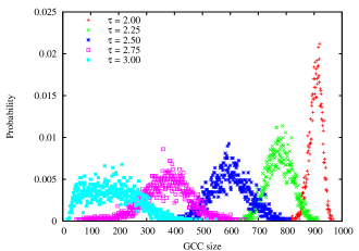
Figure 1: (Color online) Distributions of GCC sizes ($n_{\mathrm{GCC}}$).

Another source of difficulties concerning Eq. (11) is that it depends on the distribution of a node’s immediate descendants on BFS trees (i.e., $P_{c}$ for $c\geq 0$), which to our knowledge cannot be determined analytically with satisfactory correctness or accuracy . What we do is to resort to simulation data to fill in for this distribution, but even this has to be approached carefully, for reasons that are apparent in Fig. 2. In this figure, the distribution of immediate BFS descendants within the GCC is shown for three values of $\tau$ and two values of $n$. For fixed $\tau$, the distribution seems to be the same (except for variations due to finite-size effects) for both $n=1\,000$ and $n=10\,000$. So, although all our simulations are carried out for the smaller of these values of $n$, we use simulation data relative to the larger one, since the effects of finite $n$ only become manifest for significantly higher degrees.

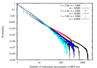
Figure 2: (Color online) Distribution of immediate BFS descents.

We remark, in addition, that this use of simulation data in lieu of the distribution called for in Eq. (11) may itself be prone to severe inaccuracy because of the already mentioned dependency on $\tau$ of the GCC-size distribution. For the larger values of $\tau$, the fact that GCC sizes are widely varying implies that any number giving a node’s immediate BFS descent is necessarily highly dependent on the size of the current GCC. Ideally, we should express such numbers as fractions of $n_{\mathrm{GCC}}$ (as in fact we do in Section IV for other quantities), but this would require—in place of Eq. (11)—an expression in terms of such fractions as well. Regrettably, we have no such expression just yet.

IV Computational results and discussion

Our computational results are summarized in Figs. 3 and 4 for five values of $\tau$ in the interval $[2,3]$. Fig. 3 gives the descent distributions and also their analytical predictions as given by Eq. (11). Since no descent value is larger than the GCC size ($n_{\mathrm{GCC}}$) for the graph in question, all data are shown normalized to the appropriate $n_{\mathrm{GCC}}$: simulation data are normalized to the corresponding GCC sizes occurring during the simulation, and analytical data to the mean GCC size for the $\tau$ value at hand.

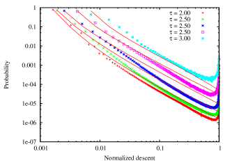
Figure 3: (Color online) Descent distributions. Solid lines give the analytical predictions of Eq. (11). Abscissae are normalized to $n_{\mathrm{GCC}}$ and binned.

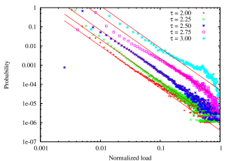
Figure 4: (Color online) Load distributions. Solid lines give power laws of exponent $-2.2$. Abscissae are normalized to $n_{\mathrm{GCC}}^{2}$ and binned.

Notice that all simulated probabilities accumulate significantly at the largest possible normalized descent. While this is clearly due to the finiteness of $n$, for $\tau\leq 2.75$ it also indicates that, had we been able to afford substantially larger values of $n$, we could expect this accumulated probability to spread through values of normalized descent one to two orders of magnitude below the maximum and make the simulation data agree with the analytical predictions ever more closely from below. As we discussed in the previous section, this is in good agreement with the limitations we expect Eq. (11) to have for relatively small values of $n$. As for the remaining value of $\tau$ ($\tau=3$), recall that in this case the effect of relatively small $n$ is considerably severer, since $n_{\mathrm{GCC}}$ has a very low mean and is also very widely spread. So, while we may still expect good agreement between simulation and analytical data as $n$ grows, this seems to be reasonable only for values of $n$ even larger than for the previous $\tau$ values.

All the simulation data in Fig. 4 are also normalized, but now to $n_{\mathrm{GCC}}^{2}$, since the greatest load value a node may have grows quadratically with the number of nodes . These data are plotted against power laws of exponent $-2.2$, which is the exponent that in Goh et al. (2001) is conjectured to be universal with respect to $\tau$ for large $n$. And in fact the agreement of these power laws with the simulation data seems good for $\tau\leq 2.5$, as in these cases GCC sizes have a relatively high mean and low spread. However, unlike the case of the descent distributions, normalizing and binning the raw simulation data for the load distributions has the deleterious effect of masking important information that is present in the raw data and allows nodal-load distributions to be interpreted in terms of the underlying descents.

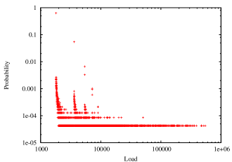
Figure 5: (Color online) Load distribution for $n_{\mathrm{GCC}}=904$ and $\tau=2$.

This is illustrated in Fig. 5, where the raw simulation data are shown for $\tau=2$ but restricted to graphs having $n_{\mathrm{GCC}}=904$, where $904$ is the observed mean GCC size. What we see in this figure is a succession of sharply defined probability peaks. The first peak occurs for a load value of $1\,807$, the second one for $3\,611$, the third for $5\,413$, and so on. If we examine these numbers in the light of Eq. (1), which expresses a node’s load as the sum of its descents in the $n_{\mathrm{GCC}}$ distinct BFS trees, then they can be explained as follows:

• The first peak’s location can be decomposed as $1\,807=904\times 1+1\times 903$, and therefore accounts for those nodes whose descent is $904$ in exactly one tree (this happens for every node and corresponds to the tree rooted at it) and $1$ in all the remaining $903$ trees (of which they are leaves). These, clearly, are all degree-$1$ nodes. Note also that the trees in which they have descent $1$ constitute the near totality of the trees.

• The location of the second peak can be similarly decomposed, for example as $3\,611=904\times 1+903\times 1+2\times 902$, referring to those nodes whose descent is $904$ in the tree rooted at it, is $903$ in one other tree, and $2$ in the remaining $902$ trees. There may exist degree-$2$ nodes that conform to this arrangement of descents, but this is no longer necessary. Also, now it is the trees in which these nodes have descent $2$ that constitute the overwhelming majority of the trees.

• For the third peak, we can write $5\,413=904\times 1+903\times 2+3\times 901$, now referring to nodes that have descent $904$ in the tree where it is root, $903$ in two other trees, and $3$ in the remaining $901$ trees. Once again it is possible, though not necessary, for this arrangement to refer to degree-$3$ nodes. Continuing the trend established by the previous two cases, the trees in which they have descent $3$ are by far the most numerous.

This same pattern of “diophantine” decomposition can be applied to the subsequent peaks and, although the correspondence to node degrees beyond $1$ is not guaranteed, we see that peak locations tend to become chiefly determined by the descents which, from our previous analyses, we know are the most frequently occurring: $1$, then $2$, then $3$, etc.

As for larger values of $\tau$, we remark that the same type of behavior can also be observed, provided $\tau$ is sufficiently small for GCC sizes to be relatively large and concentrated around the mean.

V Concluding remarks

We have considered the load of nodes in scale-free networks and have studied its distribution from the perspective of expressing a node’s load in terms of the node’s descents in all BFS (or shortest-distance) trees in the graph. We have characterized the descent distribution semi-analytically by resorting to a generating-function formalism and to simulated data on the distribution of immediate BFS descendants. We then studied the distribution of nodal load, but through computer simulations only (analytical work in this case would require independence assumptions that we found to be too strong).

Our results have allowed us to revisit the results of Goh et al. (2001) on the load distribution, particularly the conjecture that such a distribution is a power law whose exponent does not depend on $\tau$ (i.e., is independent of the underlying graph’s degree distribution in the scale-free case). The purported universal exponent of the load distribution is $-2.2$, and indeed we have been able to confirm that such an exponent seems satisfactorily accurate for large networks after data have been conveniently normalized and binned.

Looking at the raw data, however, reveals that the load distribution is richly structured in a way that can be understood precisely by resorting to the characterization of nodal load in terms of descents in BFS trees. In our view, this discovery indicates that nodal load is not power-law-distributed and that the conjecture of a universal exponent makes, after all, little sense. Of course, the origin of the previously accepted conclusion and conjecture seems to have been the mishandling of data by inappropriate binning. This, along with other pitfalls of a similar nature, is often the source of inaccurate data interpretation Clauset et al. (2007).

We note, finally, that studying quantities like descents in trees and nodal load is well aligned with what we think should be the predominating direction in complex-network investigations. The overwhelming majority of network studies so far have concentrated primarily on structural notions of a predominantly local nature (e.g., node-degree distributions). Descents and loads, on the other hand, are examples of structural notions of a more global nature and, for this very reason, their study constitutes an important step toward complex-network research that emphasizes the networks’ functional, rather than structural, properties.