Modeling Ultraviolet Wind Line Variability in Massive Hot Stars
Abstract
We model the detailed time-evolution of Discrete Absorption Components (DACs) observed in P Cygni profiles of the Si iv 1400 resonance doublet lines of the fast-rotating supergiant HD 64760 (B0.5 Ib). We adopt the common assumption that the DACs are caused by Co-rotating Interaction Regions (CIRs) in the stellar wind. We perform 3D radiative transfer calculations with hydrodynamic models of the stellar wind that incorporate these large-scale density- and velocity-structures. We develop the 3D transfer code Wind3D to investigate the physical properties of CIRs with detailed fits to the DAC shape and morphology.
The CIRs are caused by irregularities on the stellar surface that change the radiative force in the stellar wind. In our hydrodynamic model we approximate these irregularities by circular symmetric spots on the stellar surface. We use the Zeus3D code to model the stellar wind and the CIRs, limited to the equatorial plane. We compute a large grid of hydrodynamic models and dynamic spectra for the different spot parameters (brightness, opening angle and velocity). We demonstrate important effects of these input parameters on the structured wind models that determine the detailed DAC evolution.
We constrain the properties of large-scale wind structures with detailed fits to DACs observed in HD 64760. A model with two spots of unequal brightness and size on opposite sides of the equator, with opening angles of 20 5 and 30 5 diameter, and that are 205% and 85% brighter than the stellar surface, respectively, provides the best fit to the observed DACs. The recurrence time of the DACs compared to the estimated rotational period corresponds to spot velocities that are 5 times slower than the rotational velocity.
The mass-loss rate of the structured wind model for HD 64760 does not exceed the rate of the spherically symmetric smooth wind model by more than 1%. The fact that DACs are observed in a large number of hot stars constrains the clumping that can be present in their winds, as substantial amounts of clumping would tend to destroy the CIRs.
1 Introduction
Over recent years compelling evidence has accumulated that the mass-loss rates of hot massive stars have systematically been overestimated because their winds are not simply steady outflows of stellar material, but frequently contain complex density- and velocity-structures. There is considerable observational evidence that hot star winds are clumped both on small and large length scales. The presence of structure significantly influences the mass-loss rate determinations (Fullerton et al., 2006; Prinja et al., 2005; Puls et al., 2006). This in turn is important for models of stellar and galactic evolution.
Hydrodynamic models by Cranmer & Owocki (1996) showed that large-scale (or coherent) wind structures in the form of Co-rotating Interaction Regions (CIRs) can at least qualitatively explain the behavior of Discrete Absorption Components (DACs) in UV resonance lines of hot stars. The DACs are observed to propagate bluewards through the line profiles on time scales comparable with the stellar rotation period (e.g. Massa et al., 1995a; Prinja, 1998). The CIRs are spiral-shaped density and velocity perturbations winding up in or above the plane of the equator that extend from the stellar surface to possibly several tens of stellar radii. CIRs can be produced by intensity irregularities at the stellar surface, such as dark and bright spots, magnetic loops and fields, or non-radial pulsations. The surface intensity variations alter the radiative wind acceleration locally, which creates streams of faster and slower material through the extended stellar wind. The CIRs are formed where the fast and slow wind regions collide.
In this paper we investigate to what extent the CIR wind model can explain the detailed wind line variability observed in the B0.5 Ib supergiant HD 64760. Fullerton et al. (1997) pointed out how exceptional IUE data have made this (apparently single) field star ( 4.24) a key object for studying the origin and nature of variability in hot-star winds. For this star there is a substantial amount of high-quality IUE observations (MEGA campaign, Massa et al., 1995a) with unsaturated P Cygni profiles we utilize to model wind regions where the CIRs dominate the dynamics. Fullerton et al. (1997) propose to clearly distinguish the slowly bluewards shifting DACs from a second type of wind line variability called ‘modulations’. The latter are most pronounced at intermediate blueshifts and drift fast. They are not ‘discrete’ absorption components, but are very broad and rather shallow. We do not investigate the modulations here, but we refer to Hamann et al. (2001), Brown et al. (2005) and Krtička et al. (2004) who provide kinematical models for these modulations. Owocki et al. (1994) present a model specifically for HD 64760.
We focus instead on the detailed DAC properties with fully hydrodynamic models. We extend the work of Cranmer & Owocki (1996) by using CIR models to obtain a best fit of the DAC evolution for HD 64760. The star has a high rotational velocity, suggesting we see it close to equator-on (in what follows, we will assume that ): this will considerably simplify the modeling of the CIRs and the comparison to the observations.
Kaufer et al. (2006) investigate variability observed in optical lines of HD 64760 and propose a model with perturbations (spots) resulting from the interference of non-radial pulsations at the base of the wind. This interference pattern does not co-rotate with the stellar surface. In this paper we show that the shape and evolution of the slow DACs observed in UV wind lines, such as Si iv 1395, of HD 64760 can correctly be computed with a spot velocity different from the stellar surface velocity. The requirement that the CIRs originate from spots that are not locked onto the surface turns out to be crucial for the development of more realistic hydrodynamic models of large-scale wind structures in massive hot stars.
In fitting the HD 64760 observations, we concentrate on the apparent acceleration of the DAC (i.e. the evolution of the velocity position of the flux minimum with time) and the morphology (DAC FWHM evolution over time). Using a kinematical model, Hamann et al. (2001) showed that the apparent acceleration of DACs is always steeper than derived from non-rotating wind models with the same velocity law in the radial direction. For spots locked to the surface they concluded that the DAC acceleration does not depend at all on the stellar rotation rate. The present work allows us to check if this conclusion still holds for spots not locked on the surface.
We implement an advanced 3D radiative transfer code Wind3D for the detailed modeling of the properties of radiatively driven winds (Sect. 2.1 and Appendix). It solves the radiation transport problem in three geometric dimensions for winds with arbitrary density models and velocity fields. The transfer modeling assumes that the line under consideration is a pure scattering line (which is an important ingredient of non-LTE) for calculating its detailed shape formed in a supersonic accelerating wind. We investigate the physics of dynamic wind structures by analyzing HD 64760 both observationally (Sect. 3) and theoretically (Sect. 5). We compute an advanced hydrodynamic model and perform radiative transfer calculations in its rotating wind. We explore models with structured wind regions that either co-rotate with the stellar surface, or rotate slower than the surface (Sect. 4). We compare time series of theoretical line profiles (‘dynamic spectra’) with detailed spectroscopic observations of the Si iv 1395 line variability. In Sect. 6 we discuss some physical properties of the large-scale structured wind regions (mass-loss rate and dynamic properties) that result from our best fit procedure. We address the important question of how much additional material the structured wind contains compared to spherically symmetric smooth wind models. We also compare our results to the Kaufer et al. (2006) model for H variability in HD 64760. The summary and conclusions are given in Sect. 7.
2 Numerical Wind Modeling
2.1 3D Radiative Transfer Code Implementation
We develop the computer code Wind3D for the spatial transfer of radiation in optically thick resonance lines observed in massive star spectra. Our implementation is based on the finite element method described by Adam (1990). In the Appendix we present the implementation of the 3D radiative transfer scheme by further developing Adam’s Cartesian method with three new aspects. (i) We considerably accelerate the 3D lambda iteration of the source function with appropriate starting values computed with the Sobolev approximation. (ii) Since the lambda iteration is the bottleneck of the numerical transfer problem we fully parallelize the mean intensity computation. (iii) We introduce a new technique that 3D interpolates the converged source function to a higher resolution (spatial) grid to solve the final 3D transfer equation for very narrow line profile functions. It enables us to resolve small flux variations in the absorption portions of very broad unsaturated P Cygni line profiles.
In the following sections we apply Wind3D to model the profiles of the Si iv 1395 line of HD 64760 and investigate the effects of large-scale wind structures on the detailed variability of the emergent line fluxes. We model only the short-wavelength component of this doublet resonance line. We can do this as the lines are well separated because the terminal velocity (=1500 ) is not too high. The code could easily be adapted to model both components at the same time. In the next Section we test the detailed line formation calculations with models of accelerating isothermal winds that incorporate parameterized 3D density- and velocity-structures. In Sect. 2.3 we replace the input models with more realistic hydrodynamic models that invoke large-scale wind structures in the plane of the equator.
2.2 3D Parameterized Wind Models
Preliminary tests of the Wind3D code were carried out to compare the accuracy of the equidistant 3D rectangular grid computations with a simplified radiative transfer (SEI) method. The latter method (Sobolev with Exact Integration; Lamers et al., 1987) is however limited to spherically symmetric winds which is not applicable to more realistic asymmetric wind conditions. The SEI method, however, offers a simplified line source function, critical for very fast calculations of the detailed shape of resonance lines that form in radiatively driven winds. It was therefore temporarily adopted to test the numerical accuracy and efficiency of Wind3D. Over following code implementation stages the assumptions of a smooth and symmetric wind were relaxed to the more realistic conditions of structured asymmetric winds. The simplified SEI source function was therefore replaced with the fully lambda-iterated line source function.
The Wind3D code very efficiently computes the transport of radiation in detailed spectral lines formed in extended stellar winds. The FORTRAN code is developed for high-performance computers with parallel processing. It has been implemented as a fully parallelized (exact) lambda iteration scheme with a two-level atom formulation. We also implemented and tested an accelerated lambda iteration scheme (ALI), but which turned out to not significantly accelerate the overall convergency rates for pure scatting lines formed in optically thin wind conditions (see discussion in Appendix B). Applications of Wind3D to wind conditions that are much more optically thick will be given elsewhere. The model calculations are performed with grid-points on an equidistant grid. The code lambda-iterates the 3D line source function to accuracies below 1% differences between subsequent lambda iteration steps. The local mean intensity integral sums 80 80 spatial angles over 100 wavelength points covering the P Cygni profile. Next the source function is interpolated to grid-points and the 3D radiative transfer equation is solved to determine the emergent flux. Both during the lambda iteration and in the final radiative transfer equation, the intrinsic line profile function is assumed to be a narrow Gaussian function.
Tests with spherically symmetric models show that the 1 % constraint on the difference between subsequent lambda iteration steps results in a final source function that is very close to the SEI solution. However, more important for our detailed modeling purposes is the effect on the resulting line fluxes. We find that these differ by less than in the flux normalized absorption portion of the P Cygni profile. Lambda iterating to 0.1% (or 0.01%) therefore yields identical emergent flux profiles, but lengthens iteration times tremendously. We emphasize however that the emergent line fluxes we compute strongly depend on the very narrow intrinsic line profile width of only 8 we adopt. Our grid of points for the line source function undersamples the narrow line profile function . For the actual line flux calculations we therefore have to refine the grid to at least points, to avoid an undersampling of . We 3D-interpolate the iterated line source function values to this higher-resolution grid (see Appendix C). Lower-resolution grids would result in line profiles that are too (numerically) noisy to compare with the observations.
Wind3D has been carefully load balanced for parallel processing with the OpenMP programming strategy, and shows excellent scaling properties for multi-threading. It accepts arbitrary 3D density models and velocity fields without assumptions of axial symmetry. As it uses an observer frame approach, complicated code constructs to track multiple resonance points are avoided. Wind3D is ‘fast’ and very accurate to trace small variations of local velocity gradients and density on line opacities in strongly scattering dominated extended stellar winds. It currently runs on a parallel compute server with 64-bit Itanium-2 1.5 GHz microprocessors and a memory architecture allowing for very fast access to all the memory on the server. A typical run ( mesh, angles, 100 wavelengths) for a single spectral line with ‘normal’ convergence rates of the source function takes 300 min of wallclock time using 16 CPUs, followed by another 300 min to interpolate the source function ( gridpoints), and to compute the dynamic spectrum over 36 lines of sight. We discuss some memory allocation and parallelization properties in Appendices B & C.
We test Wind3D with parameterized input models of the wind-velocity and -opacity. We consider a -velocity law for an isothermal wind with =1 and =35 . The underlying smooth wind reaches a terminal velocity of =1600 within the simulation box of 30 . The smooth wind is perturbed with 3D spiraling density structures wound around the central star (the velocities are unchanged from their smooth-wind values). The source function in the structured model is 3D lambda-iterated to equilibrium with the radiation field of the structured wind. The convergency of the iterations can be accelerated but our tests show that it is already fast and converges within 5 to 8 iterations when the size of the CIRs above and below the plane of the equator is limited to 0.5 at the outer edge. The converged 3D line source function is used to solve the transfer problem for a uniformly distributed set of sight-angles in the plane of the equator around the star. In the test input models important free parameters for our detailed line profile modeling are therefore the properties of the adopted 3D wind structures, such as the number of spiral arms, their curvature and width, the height (or flaring angle), the density contrast profile throughout the spiral arms, and the inclination angle of the observer’s line of sight in or above the equatorial plane.
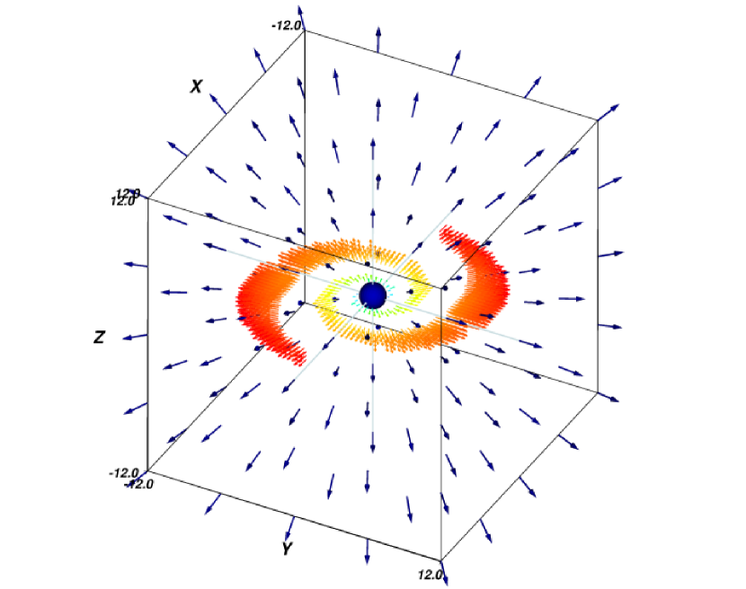
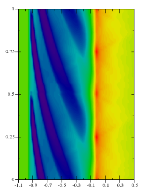
Parameterized 3D models of Co-rotating Interaction Regions (CIR) already provide comprehensive comparisons to the DAC evolution observed in resonance lines of massive hot stars. Figure 1 shows a schematic drawing of a parameterized wind velocity grid with two CIRs in the shape of winding density spirals. The smooth wind expansion is spherically symmetric with a beta-power velocity law (outer arrows). The wind velocities inside the CIRs also assume the beta law of the ambient wind and are directed radially (velocity vectors drawn with much finer spacing in the equatorial plane). The widths of both CIRs increase outwards with an exponential curvature. The outer edges of the CIRs are truncated at a maximum radius of 12 . Figure 2 shows the dynamic spectrum computed with Wind3D for the structured wind model in Fig. 1. The computed line profiles reveal two (and for certain rotation phases three) Discrete Absorption Components (DACs) drifting toward shorter wavelengths in the unsaturated absorption trough of the P Cygni line profile (time runs upward). The time sequence of these line fluxes is shown in the right-hand panel in grey-scale. The line opacity () inside the CIR has been increased by one order of magnitude with respect to the surrounding smooth wind opacity. The dynamic spectrum is computed for 72 angles of sight in the plane of the equator around the star. The Figure shows that the widths of the DACs decrease while they asymptotically drift toward shorter wavelengths. The DACs shift toward the blue edge of the P Cygni profile because the observer probes regions of increased wind absorption inside the CIR at larger distances from the star as the entire CIR structure rotates through the line of sight. The widths of the DACs decrease because the range of (radial) velocities in the CIR projected in the observer’s line of sight (inside the absorbing cylinder in front of the stellar disk) decreases at larger distances from the star. At large distances from the star a radially expanding spherically symmetric wind has a smaller dispersion of radial velocities projected into the line of sight for the wind volume in front of the stellar disk. In Sect. 4.3.2 we investigate the DAC line formation with advanced hydrodynamic models in which both the CIR density and resulting wind velocity gradients turn out to be important for the detailed DAC evolution.
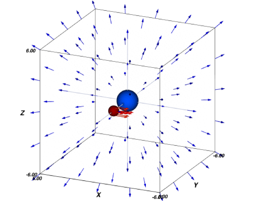
Further 3D transfer tests with parameterized spherical wind perturbations (‘blobs’ or ‘clumps’) of denser gas that move in front of the star produce extra and less absorption at different wavelengths in the wind profile. In Fig. 3 the opacity in the clump has been increased by an order of magnitude compared to the ambient wind opacity. The clump passes in front of the stellar disk and partly obscures it. It moves perpendicular (tangentially drawn arrows) to the surrounding radially expanding wind (outer arrows) which enhances the line absorption around the rest velocity (small dips in the line emission lobe). The dynamic spectrum in Fig. 4 shows how the absorption portion of the P Cygni profile becomes weaker when the local opacity enhancement in the blob crosses the observer’s line of sight. However, the amount of photon scattering between the star and the observer also decreases because the blob removes a region in the wind where resonant scattering would occur at the velocity of the surrounding wind (as the blob moves perpendicular to the radial wind expansion in the model). Around 70 % of the wind scattering therefore diminishes, yielding somewhat larger line fluxes in the absorption portion of the P Cygni profile (small bumps in the absorption trough). The clump diminishes the amount of line absorption in the line profile of Fig. 4, but also the line re-emission. For a given line of sight the decrease of absorption due to the blob does not have to equal the decrease of emission. When the clump is located in front of the star the“loss of absorption exceeds the loss of emission since absorption of photons is re-emitted into 4 . Other calculations with Wind3D show how the line absorption decreases further with larger clump opacities and larger clump sizes. The distance of the clump to the star determines the precise velocity position of the flux bump since the wind accelerates radially. In this example the velocity position of the small flux bump is (almost) invariable because the smooth wind velocity profile is spherically symmetric and the clump moves at the same distance from the star through the wind for an observer in the plane of the equator.
It is not a priori clear if a fully self-consistent line source function calculation is required in our modeling. We are, after all, not concerned with detailed changes in the relative depth of DACs (our best fit procedure is based on the DAC shape and FWHM evolution), and far blue-shifted DAC absorption chiefly results from line opacity in the wind volume in front of the stellar disk. When the volume in this cylinder is relatively small compared to the total wind volume its emission can safely be neglected with respect to the contributions from the emission lobes. Since the height of our hydrodynamic wind models is only 1 around the plane of the equator, having almost strictly radially expanding wind structures, there is no far blue-shifted emission emerging from the emission lobes that can significantly alter the small DAC absorption. It is however not correct to assume that an iteration of the source function in 3D radiative transfer calculations can be neglected for detailed modeling of wind features observed in any type of spectral line. A stronger underlying P Cygni profile would be influenced more by the emission, which could start to “erase” the DAC at lower velocities. Also, when the absorption features occur at much smaller velocities (around stellar rest say), and the hydrodynamic structures yield far blue-shifted emission, the detailed source function of the structured wind cannot be neglected. This is for instance the case for the double-peaked emission lines formed in Be-star disk winds, or for the wine-bottle type H emission profiles modeled by Hummel (1992). The study of the physical properties of large-scale structures in winds of massive hot stars is not limited to UV resonance lines only. The H profile of HD 64760 (Kaufer et al., 2006) reveals symmetrically blue- and red-shifted emission humps with 2.4 d modulations that can result from variations at the base of the stellar wind. It remains to be studied how 3D radiative transfer modeling of H can be combined with hydrodynamic models of rotational modulations observed in the Si iv line (but not addressed in this paper). It is clear however that to compare detailed normalized fluxes of both lines a self-consistent calculation of the H and Si iv line source functions in the structured wind model is required.
2.3 Hydrodynamic Wind Models
Our approach of computing hydrodynamic CIR models is very similar to that of Cranmer & Owocki (1996). The main differences are that we utilize the Zeus3D111http://www.astro.princeton.edu/jstone/zeus.htm (Stone & Norman, 1992) code rather than the VH-1 code, and that we introduce a spot velocity that does not have to equal the stellar rotational velocity.
We first outline the procedure and summarize the assumptions that we share with Cranmer & Owocki. The time-dependent 3D equations of hydrodynamics are solved, limited to the equatorial plane of the star. Full 3D hydrodynamic calculations of CIRs have been presented by Dessart (2004) and these suggest that 3D effects are small for spots that are symmetric around the equator. We opted to limit our calculations to the equatorial plane as the gain in computing time allows us to more fully explore the parameter space.
Our models include the rotation in the equatorial plane of the star, the gravity acceleration (corrected for electron scattering), and the line force due to radiative driving by line scattering. For evaluating the line force we apply the local Sobolev approximation and the CAK parameterization using a finite-disk correction. Note that this approach neglects the diffuse radiation field, which also suppresses the line-driven instability. It allows us to investigate the effect of the large-scale CIR wind structures rather than small-scale structures due to instability. For the Sobolev approximation we apply the absolute value of the radial velocity gradient (Rybicki & Hummer, 1978), while we neglect any multiple resonance points due to the possibly non-monotonic wind velocity. Although HD 64760 is a rapidly rotating supergiant we neglect possible effects of gravity darkening and rotational oblateness on the star and its wind. Limb darkening is also neglected. We include only the radial component of the radiative force in our model.
The neglect of non-radial forces, gravity darkening and oblateness could be relevant for the mass loss rate in the equatorial plane. Owocki et al. (1996) have shown how material can flow poleward if these effects are included (contrary to what might be expected from the Wind-Compressed Disk model – Bjorkman & Cassinelli (1993)). The mass-loss in the equator could therefore be smaller than the published value.
In our hydrodynamic model, one or more local radiation force enhancements (‘spots’) can be introduced at the base of the stellar wind. Each spot is determined by its position at time on the stellar surface, spot rotation velocity , spot strength (or brightness), and opening angle (the diameter of the spot). The spot is assumed to be circular symmetric and centered on the equator. Only the radial component of the additional line force due to this spot is included in the model. The additional force is responsible for the structure in the wind. The line force takes into account the full extent of the spot (i.e. not only the part on the equator but also those parts above and below it). The force is calculated analytically for any point directly above the spot center (including limb darkening in the spot). For other positions it is assumed that a Gaussian function (of azimuthal angle) relates the line force there to that directly above the spot center; this assumption is made to reduce computation times. For detailed equations we refer to Cranmer & Owocki (1996).
Our hydrodynamic modeling also includes radiative cooling in the energy conservation equation. Radiative heating has not been implemented, but instead a floor temperature is adopted to prevent the wind material from cooling down to below 80% of the stellar effective temperature. However, in the models presented in this paper this cooling turned out to be unimportant and all models are isothermal at 0.8 . We find in our exploratory calculations that this is no longer true for very bright spots (brighter than is required for modeling HD 64760). As an example, for = 20° and , the wind is no longer isothermal due to shock heating. The boundary value for where shocks become important is dependent of the spot angle and velocity. We find however that the wind is isothermal for all models with .
The main difference in our modeling with Cranmer & Owocki (1996) is that we allow the (angular) velocity of the spot rotation to differ from the velocity of the rotating stellar surface ( ). This is based on two arguments. Firstly, Kaufer et al. (2006) have shown that a beat pattern of non-radial oscillations (in HD 64760) can produce local surface spots required for modeling the large-scale wind structures. The beat patterns, however, are not locked onto the stellar surface, but can rotate with a velocity different from the stellar rotational velocity. Secondly, the observed recurrence time scale of the DAC compared to the estimated rotation period (Sect. 5) demonstrates that spot velocities considerably different from the surface velocity are required to match the observations. By abandoning the usual assumption that equals a much wider range in the dynamic behavior of the large-scale wind structures emerges from the models.
We have thoroughly tested the new hydrodynamic code and can successfully reproduce the results of Cranmer & Owocki (1996). We tested that the results of the code are not sensitive to details, such as the number of points in the grid, the extent of the grid, the Courant number and the assumed floor temperature. The results are slightly sensitive to the order of the advection scheme that is used (by default we use a second-order scheme), but the effect is not large enough, however, to influence the conclusions of this paper.
The stellar and wind parameters of HD 64760 were adopted from Kaufer et al. (2006) and are listed in Table 1. Note that these parameters are in acceptable agreement with the more recent ones derived by Lefever, Puls, & Aerts (2007). We determine the CAK and parameters to obtain the observed mass-loss rate and the terminal wind velocity (for simplicity, we assumed the CAK parameter ). We apply a polar grid in the hydrodynamic calculations. 800 grid points sample the radial direction covering the wind range 1–30 . The grid-step increases by a fixed ratio from the inside to the outside of the radius grid. For the angular part 900 spatial angle points are uniformly distributed over the full range. We set the Courant number to 0.5. The initial conditions of the model start with an angle-independent smooth wind flow having a -velocity law with the observed . The density structure of the smooth wind is derived from the conservation of mass and the observed mass loss rate. During the initial part of our hydrodynamic calculations the smooth wind settles into a stable steady-state outflow that becomes time-independent. Next one or more local spots are turned on at the stellar surface, yielding large-scale asymmetric structures in the extended stellar wind. We then proceed until the models assume a stationary state with a steadily expanding structured rotating wind.
The resulting equatorial density and velocity structure are then introduced into the Wind3D code. This is done by copying the structure in all planes parallel to the equatorial one, within around the equatorial plane. Outside this region, the density and velocity have their smooth wind value (as calculated by Zeus3D).
3 Observations
We investigate the detailed DAC properties in the high-resolution time series of IUE spectra of the B-type supergiant HD 64760 (B0.5 Ib), observed during the 1995 MEGA campaign (Massa et al., 1995a). Detailed analyses of the 1993 and 1995 IUE MEGA campaign data of this star have been presented in the literature. The 1993 data are thoroughly discussed in Massa et al. (1995b), while Prinja et al. (1995) and Howarth et al. (1998) present time-series analyses of both data sets. These studies however provide periods for the rotationally modulated wind variations rather than for the slower evolving DAC structures we model in this paper. Fullerton et al. (1997) presented a complete Fourier analysis of these data comparing detailed time-series of many lines individually, however also primarily focusing on the modulation periods. Only in a more recent study did Prinja et al. (2002) point out that the recurrence time scale for the (slowly migrating high-velocity) DACs is not constrained. We therefore re-analyzed the 1995 MEGA campaign data with the goal of determining an accurate recurrence time for the DACs of HD 64760.
The 1995 data sets are extracted from the IUE archive maintained at the Goddard Space Flight Center. The IUE SWP spectra cover the wavelength range from 1150 to 1975 Å with a nominal spectral resolution 10,000. The spectra were created by staff at GSFC using the IUEDAC software to combine most of the echelle orders to form a single continuous spectrum, which was placed on a uniformly spaced wavelength grid with 0.05 Å spacing. The wavelength scale calibration was improved by centering the spectra on selected interstellar lines using an echelle order-dependent correction (see also Prinja et al. (2002)). The mean signal-to-noise ratio in the continuum is typically 20 to 30 for both data sets.
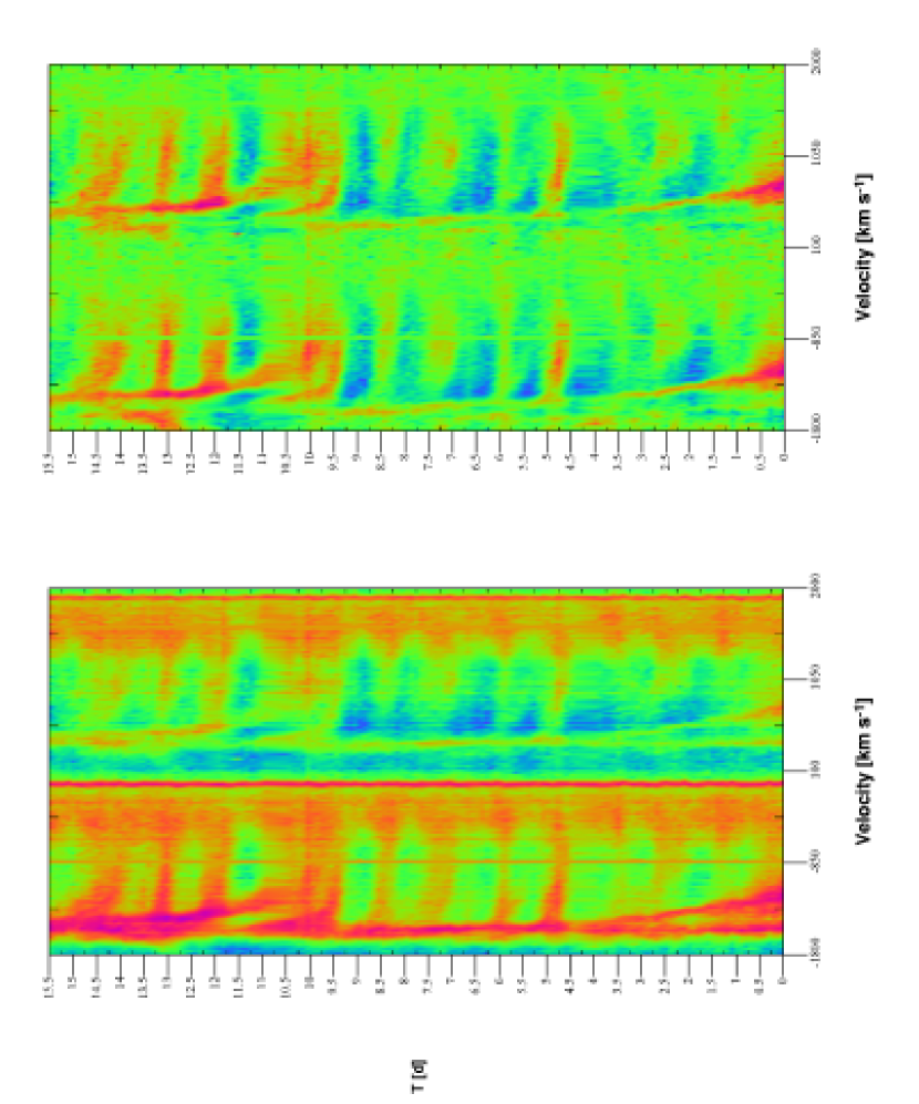
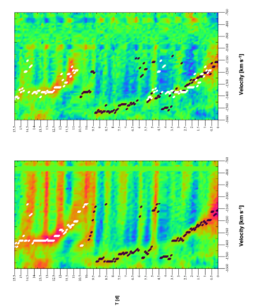
We combine a time series of 145 SWP spectra observed between 1995 January 13 at UT 12:57:35 (JD 2449731.03999) and January 29 at 01:02:18 (JD 2449746.54326). The spectra are integrated with the large aperture during 60 s, and observed about every 3 hours over this period of 15.5 d. The left-hand panel of Fig. 5 shows the time-sequence of the flux spectrum in velocity scale centered around the short-wavelength line of the Si iv 1400 resonance doublet. The dynamic spectrum is plotted with grey-scales for which dark and bright shades indicate low and high flux levels, respectively. The dark and bright shades correspond to red (or violet) and blue colors in the online image versions. The dynamic spectra in Fig. 5 are linearly interpolated over time to provide a uniform time-sampling. The dynamic spectrum reveals many subtle spectral features in the absorption portion of the P Cygni profile of both Si iv lines.
The straight vertical lines around 0 and 1900 are due to interstellar absorption of Si iv toward HD 64760. We plot the velocity scale in the stellar rest frame using a radial velocity of 41 (CDS Simbad), and a small heliocentric correction (5.43 from GSFC data header files). The flux minimum in the interstellar lines is constant within a fraction of a percent of the local continuum flux which indicates that the absolute flux calibration of the sequence is reliable. Note that the straight vertical line around 800 in the left-hand panel of Fig. 5 is due to a detector reseau mark. The zero flux values for these bins in the spectra have been set to a fixed value to prevent a compression of the grey-scale range in the dynamic spectrum image.
We investigate the Si iv lines of HD 64760 because they exhibit a variety of remarkable spectral features that signal formation in dynamic wind structures. Most striking are the slowly migrating high-velocity DACs observed between =0 and 5 d (further ‘lower DAC’), and between =10 and 15 d (‘upper DAC’) in Fig. 5. Both Si iv resonance doublet lines are sufficiently well separated. The blue edge velocity of the long wavelength P Cygni line profile does not overlap with the flux evolution of the DAC observed in the short-wavelength line. The S/N ratios in the Si iv wavelength region are sufficiently large to permit image processing techniques to the dynamic flux spectrum to investigate the detailed DAC properties without the application of any compromising spectral smoothing operations. In the right-hand panel of Fig. 5 we subtract the mean flux per wavelength bin from the absolute flux image in the left-hand panel. This operation removes the overall shape of the underlying P Cygni profiles of both doublet lines. The strong absorption feature observed around the blue edge velocity of 1600 is therefore removed in the right-hand panel of Fig. 5.
The flux difference image shows that the DACs in both doublet lines assume comparable depths and also reveal an almost identical flux evolution over time (see also the flux difference spectrum in Fig. 9 of Fullerton et al. (1997)). They drift bluewards from velocities exceeding 1000 to 1600 . The depth and width of the DACs decrease over time while drifting bluewards. The DACs are rather broad and intense when they appear in the P Cygni absorption line portion and gradually weaken and narrow while shifting bluewards. The base of the DAC evolution in HD 64760 reveals the shape of a slanted triangle over a period of 3 d. The top of the triangle further extends into a ‘tube-like’ narrow absorption feature that can be traced over the next 7 d and drifts asymptotically to a maximum velocity that slowly approaches the blue edge velocity of the P Cygni line profile. This is considerably clearer in the difference spectrum than in the original one. The flux difference spectrum clearly reveals that the lower DAC extends over time to at least 10 d.
We next constrain the recurrence time-scale for the DAC in HD 64760. For our DAC modeling purposes in Sect. 5 it is important to establish an accurate period over which the DAC recurs. In the right-hand panel of Fig. 5 we observe besides the DACs several individual spectral features that cover a large velocity range. They reveal a rather ‘bow-shaped’ morphology, extending bluewards and redwards at the same time. The ‘horizontal bow’ shape of these features clearly differs from the more ‘triangular’ shape of the DACs. These ‘modulations’ exhibit a possible period in HD 64760 of 1.2 d (Fullerton et al., 1997; Prinja et al., 2002), although careful inspection of the flux difference image reveals that these shallow modulations alternate over time with comparable absorption features that extend even more horizontally (i.e. they are almost completely horizontal without the rounded bow-like shape). Clear examples of both types of horizontal features are observed around 4.8 d and 6 d, and around 7.3 d and 8.5 d. Similarly shaped, but stronger modulations, occur around 12 d and 13.2 d when they distort the tube-like narrow absorption in the DAC at larger velocities. We observe that the flux differences in the bow-shaped modulations are distributed almost symmetrically around a velocity axis that is located 930 . For example, the fluxes in the modulation observed around 4.8 d decrease nearly symmetrically blueward and redward of this velocity value. We use this near-symmetry property of the bow-shaped features to remove the disturbing flux contributions from the modulations to the detailed DAC evolution, and to increase the flux contrast of the DAC. In the right-hand panel of Fig. 6 we subtract the mirror image from the left-hand panel. The velocity position of the mirror axis at 930 is determined by minimizing the flux contributions in the horizontal features observed between 11.5 d and 15 d that distort the flux values across the upper DAC.
Our mirroring flux difference procedure effectively cancels out the flux contributions from the modulations, while the fluxes inside the DAC remain unaffected (since the DAC is not observed symmetrically around the selected mirror axis). We next apply an automatic procedure to find the flux minimum for each separate spectrum. Due to our mirroring correction, this procedure will in most cases find the minimum of the DAC rather than that of a perturbing ‘modulation’ feature. The minima thus found are indicated in black (lower DAC) and white (upper DAC). In the right-hand panel of Fig. 6 we shift the upper DAC minima downwards and compute the best match with the shape of the lower DAC minima. We apply a simple least-squares minimization technique to the velocity positions of the shifted upper and the lower flux minima and find the best match for d. We hence determine a recurrence time of 10.3 d for the DAC in Si iv 1395 of HD 64760. We estimate an error bar of d on this result. It is clear from Fig. 6 that the upper DAC is not a repeat of the lower DAC. We show in Sect. 5 that a hydrodynamic wind model with two unequal CIRs provides the best fit to the shape and morphology of the lower and upper DAC.
It is of note that the detailed shape of the high-velocity DACs observed in HD 64760 strongly resembles the shape of DACs observed in the Si iv lines of Per (O7.5 III). The peculiar slanted triangular shape of the DAC base, which extends into a tube-like absorption feature, is also observed in a sequence of IUE spectra of 1991 October (Kaper et al., 1999). Interestingly these data reveal that the DACs in Per can extend to velocities considerably below the values observed for the DAC in HD 64760. In HD 64760 DAC velocities are observed only blueward of 1000 , while in Per they reach almost zero velocity, or down to the very base of the stellar wind. The foot of the DAC base in Per is nearly horizontal (e.g. the boundary where the DAC first appears is very sharp) signaling that the dynamic structures that produce the DACs can extend geometrically very far through the wind when they start to rotate into the observer’s line of sight (from almost the base of the wind to ).
In the following Sections we compute hydrodynamic models that correctly fit the detailed shape and morphology of the DACs in HD 64760. We find that the peculiar DAC shape cannot be computed with (simple) parameterized models of the wind density in Sect. 2.2. A detailed hydrodynamic model of Per will be presented in a future paper.
4 Hydrodynamic Wind Modeling
4.1 Model Example
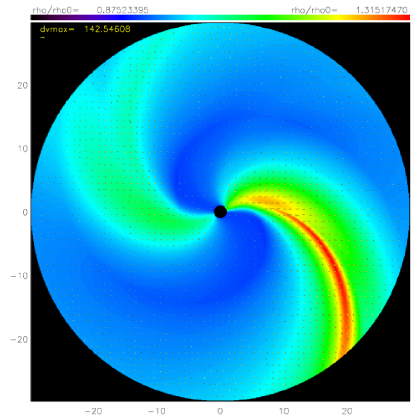
Figure 7 shows the density contrast for the hydrodynamic model222Animations of a number of hydrodynamic models are available at http://www.astro.oma.be/HOTSTAR/CIR/CIR.html of HD 64760 with , having two spots that are 20% and 8% brighter than the stellar surface (=0.2 and 0.08), with spot angle diameters of =20° and 30°, respectively. The wind velocity deceleration is typically largest inside the large-scale dynamic structures where the density contrast is also largest. This results from the conservation of momentum in the hydrodynamics equations. For an observer in the laboratory frame, wind particles expelled at the stellar surface follow almost straight radial paths outward. When the wind particles cross the spiraling structure radially they temporarily decelerate with respect to the smoothly accelerating wind, thereby enhancing the wind density locally. The extra mass from the bright spots induces stable density waves through which the surrounding fast wind streams. The density waves rotate in the plane of the equator with a period set by that of the spots. The tangential wind velocity components are small compared to the radial velocity components. They become relatively largest close to the stellar surface where the radial wind velocity is smallest. In this model the local deceleration of the flow across the density spirals does not exceed and decreases outward along the large-scale wind structures, becoming vanishingly small at radial distances beyond 30 where the density approaches that of the smooth wind expanding at .
4.2 Model Grid
To understand the effects of the different input parameters on the hydrodynamics, we compute a large grid of models with the Zeus3D code. We first compute the hydrodynamic model for the stellar parameters of HD 64760 and its smooth wind properties (Table 1). Next we introduce in the model a single spot at the equator. We vary the spot parameters of brightness (), spot angle (), and spot velocity () that provide different models for the large-scale structured wind. These models then serve as input to the Wind3D code, which calculates the resulting dynamic spectra. The underlying smooth-wind profile is subtracted from all calculated profiles to allow a comparison to the observed flux difference spectra.
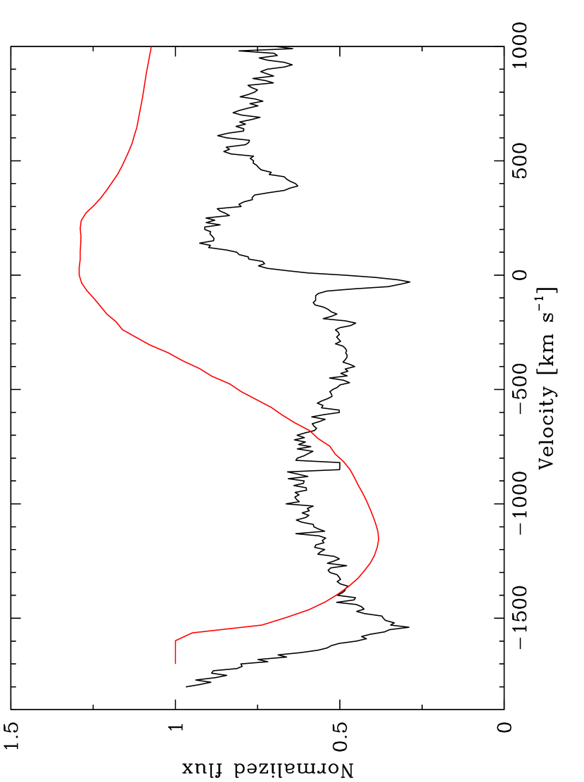
In our transfer calculations we compute the structured wind opacity in the Si iv resonance lines from the wind density contrast since / / (as long as Si iv is the dominant ion, which is the case for HD 64760). The smooth wind opacity in the lines is given by the Groenewegen & Lamers (1989) parameterization (see Appendix B). We set the thermal broadening to a small value of 8 . When the opacity parameters are set to , , , we find an acceptable “fit” to the underlying (unsaturated) P Cygni profile of the UV Si iv lines. Figure 8 shows the average normalized flux profile of the Si iv 1395 line of HD 64760 observed over a period of 15.5 d in 1995. It is of note that the Si iv line also contains other photospheric absorption lines (i.e. around 500 ), together with an interstellar absorption line (around the stellar rest velocity), a detector reseau mark, and a steady strong absorption feature around 1500 , which cannot all be accounted for in our 3D hydrodynamic wind models. We emphasize however that our DAC modeling is based on a best fit procedure in the absorption portion of the unsaturated Si iv P Cygni line profile. The best fit procedure is therefore based on the observed and computed flux difference profiles, instead of the normalized flux profiles shown in Fig. 8.
4.3 Parameter Study
In this Section we discuss the influence of the various parameters on the CIR hydrodynamics, and how the shape and morphology of the DACs in HD 64760 changes. We concentrate on the spot parameters as we assume all other parameters to be known. This parameter study will be important in Sect. 5 where we determine the best fit to the observed DACs. In doing so we concentrate on the detailed DAC shape (velocity position of the flux minima with time) and morphology (DAC FWHM evolution over time). We do not fit the detailed intensity variation of the DACs because that also depends on the opacity in wind structures above and below the equatorial plane we currently do not incorporate in our hydrodynamic models. We demonstrate however that detailed fits to the precise DAC depth are not needed primarily because the DAC shape and morphology are uniquely determined by the spot parameters.
4.3.1 Spot Strength
From the small grid of hydrodynamic models calculated by Cranmer & Owocki (1996), it is already clear that the effect of a larger spot brightness is to increase the range of density contrast (the ratio of density of the structured and the smooth wind /). The density contrast maxima increase while the minima decrease. Furthermore, the variations of the wind velocity with respect to the smooth wind velocity also increase with larger . Our more extensive grid confirms their results. For an example of a spot with and , an increase of from 0.1, 0.3, 0.6, to 1.0 increases the maximum of / from 1.5, 2.0, 5.0, to 13.7, respectively. The maximum velocity difference increases from 130 to 390 km s-1. This trend is directly related to the local increase of the total mass-loss rate the spot causes by additional radiative wind driving (see also Sect. 6). At the stellar surface the spot injects extra material into the wind that collides with smooth-wind material, thereby locally increasing the density in the resulting large-scale wind structures. The larger the spot brightness, the more material is injected into the wind, and the stronger the dynamics of this collision.
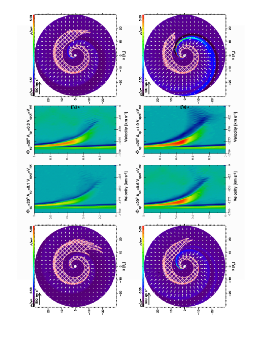
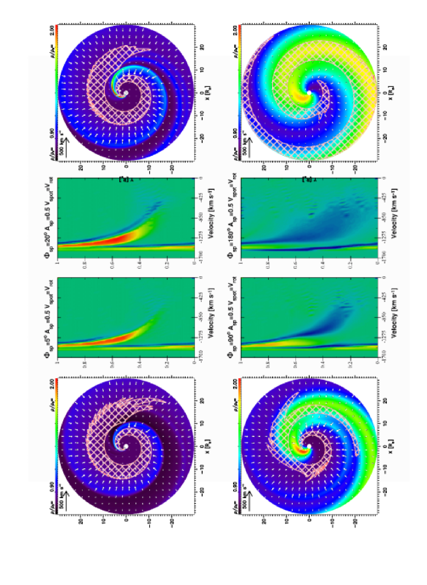
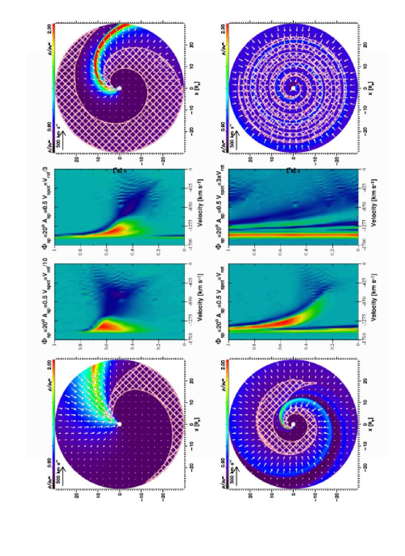
In Fig. 9 we show the effect of on the detailed DAC structure computed with Wind3D. We increase the spot intensity from 0.1 (upper left panels), over 0.3 (upper right panels) and 0.6 (lower left panels), to 1.0 (lower right panels). The spot angle =20°, while the spot velocity is set equal to the surface rotation velocity () in the four models. We plot both the hydrodynamic models and the dynamic spectra. The hydrodynamic model shows the density contrast and velocity vectors with respect to the smooth wind. The model rotates counter-clockwise over one period. The dynamic spectra show the rotation phase from 0.0 to 1.0. The rotation phase zero corresponds to the spectrum we compute for an observer in the plane of the equator viewing the rotating hydrodynamic model edge-on from the south side in these images. The flux difference profiles are shown between 0 and 1700 , which is the absorption portion of the P Cygni line profile.
4.3.2 DAC Formation Region
To study the formation region of the DAC, we introduce the “relative” Sobolev optical depth:
| (1) |
where the subscript ‘0’ refers to the smooth wind model, and we neglect the finite size of the stellar disk by considering only the central ray. DACs are formed in wind regions with large values. These regions are indicated in Figs. 9, 10, & 11 by hatched areas on the hydrodynamic plots. It follows from Eq. (1) that both the density and velocity gradients can play an important role for the formation of DACs.
As first pointed out by Cranmer & Owocki (1996), the DACs are more likely to be due to velocity plateaus than to the increased density in the CIR. The CIR causes a discontinuity in the velocity gradient (“kink”). This kink moves upstream and therefore trails the density enhancement of the CIR. The velocity plateau is bounded on one side by the kink and extends on the other side towards the CIR (see, e.g., Fig. 9). Because of the upstream movement of the kink and velocity plateau, they are more warped than the CIR. As the spot rotates, different parts of the velocity plateau cross the line of sight at increasing wind velocities. If the DAC is completely formed in the velocity plateau, this directly translates to the DAC drifting toward larger velocities. Because of the strong spiral winding, the DAC velocity increases only slowly with time, which explains the slow apparent acceleration of DACs (see also Hamann et al., 2001).
Our results confirm that DACs are mainly formed in the velocity plateau. As an example, consider the upper right-hand panel of Fig. 11. The dynamic spectrum shows a DAC that persists over the whole cycle (starting at low velocities around phase 0.25 and then narrowing with increasing phase until it disappears around phase 1.3). The hydrodynamic plot, however, shows a CIR that persist only over somewhat more than a quarter of the cycle. The density enhancement in the CIR can therefore not be responsible for the DAC. Looking in more detail we find, e.g., that at phase 0 the DAC is present around . On the hydrodynamic plot there is no density enhancement at all around phase 0 (south direction). The large Sobolev optical depth (hatched area) at this phase is due to the small value of the velocity gradient (i.e. a velocity plateau).
However, in certain cases it is the CIR density enhancement that creates the DAC. We again refer to the example of the upper right panel of Fig. 11. A more detailed study of this case shows that the relative Sobolev optical depth () is dominated by the density enhancement when the DAC is at low velocities (phases 0.25-0.5). At larger velocities, the velocity plateau dominates in the formation of the DAC.
An important aspect of the hydrodynamic models is that an increase of (all other model parameters being equal) enhances the density contrast / inside the CIR and decreases the corresponding radial wind velocity gradient behind the CIR (i.e. the wind regions between the stellar surface and the CIR). An increase of over the four models in Fig. 9 causes the CIR with large to occur farther away from the stellar surface and its overall curvature to diminish. The wind region with large also shifts farther away from the denser CIR. In regions where is small the local outflow velocity close to the stellar surface considerably decreases because of the larger density inside the CIR. For this reason strong DAC absorption in the dynamic spectrum extends further towards smaller velocities when the spot strength increases.
The radial approximation we introduced in Eq. (1) only provides an estimate of the DAC line formation depth. It breaks down in wind regions where non-radial velocities are large compared to the overall radial wind expansion. We emphasize however that the DACs we compute in the dynamic spectra with Wind3D do not utilize the radial approximation. Furthermore they also include the effect of a (small) intrinsic Doppler broadening in the source function and therefore go beyond the Sobolev approximation. The line source function in the transfer is fully 3D lambda iterated to self-consistency with the radiative transfer equation to compute the detailed DAC fluxes.
4.3.3 Spot Opening Angle
Cranmer & Owocki (1996) conclude from their hydrodynamic models that the maximum density decreases with increasing spot angle () with the exception of the smallest , where they presume to have undersampled the wind structure. Our more extensive grid (also calculated at a higher spatial resolution) shows a clearer picture. For small spot angles, the range in density contrast and the velocity differences increase with increasing spot angle. This is consistent with the idea that larger spot angles also increase the amount of mass injected into the surrounding stellar wind. Towards even larger spot angles, however, the larger density contrast and velocity differences begin to level off and to decrease (consistent with the findings of Cranmer & Owocki). An example with and shows that the maximum / varies from 1.2, over 3.8, down to 1.9 when increases from 5° over 20° to 180°. The decrease of / with larger results from the larger angular extent over which the extra mass injected by the spot spreads out, which makes its collision with the ambient smooth wind material less efficient (also noted by Cranmer & Owocki).
In Fig. 10 we increase the spot opening angle from 5°, over 20° and 90°, to 180°. The spot co-rotates with the stellar surface, and =0.5. We find that an increase of the spot angle considerably alters the FWHM evolution of the DAC. The DAC base strongly broadens when increases from 20° to 90° because extra wind material injected by the spot becomes more spread out over the plane of the equator. The maximum of in the CIR occurs within 5 above the stellar surface. Inside this region the extra wind material is distributed over a larger geometric region above the bright spot (and surface), which also considerably broadens the density contrast in the tail of the CIR. When this region rotates in front of the stellar disk (around rotation phase 0.2 in the lower right-hand panel) the DAC base becomes much broader because the range of velocities projected in the observer’s line of sight (that contribute to the DAC opacity) strongly increases (see Sect. 2.2). Note that the wind flows almost radially through the CIR density structure near the surface (where particles decelerate as they approach and cross the CIR and accelerate again once they have passed it) with rather small tangential components. It is however the range of projected radial velocities in front of the stellar disk that determines the total width of the DAC base. We find that the Sobolev approximation that only includes strictly radial velocity gradients yields line formation regions in the hydrodynamic models (hatched regions in Fig. 10) that do not correspond with the actual DAC formation regions when the tangential wind velocity components cannot be neglected.
4.3.4 Spot Rotation Velocity
The winding of the large-scale structures in the hydrodynamic models (i.e. the number of turns of the spiral arm in the equatorial plane around the central star) largely depends on the spot velocity (for fixed ). The spiral winding increases when the spot velocity increases with respect to the surface rotation velocity. Much smaller effects on the spiral winding are due to the spot angle; the spiral winding decreases somewhat when the spot angle increases.
In Fig. 11 we compute the DAC for a spot rotation velocity that increases from /10, /3 and , to , with =0.5 and =20°. When the spot rotation trails the surface rotation, the curvature of the CIR considerably decreases (upper panels). For =/10 the density contrast in the CIR has the shape of a somewhat curved sector in the equatorial plane. When this sector rotates through the observer’s line of sight (around rotation phases of 0.6-0.7), becomes small over a wind region that extends from the base of the wind (close to the surface) to the outmost wind regions beyond 30 in the hydrodynamic model (hatched area in the upper left-hand panel). The DAC forms over the entire wind region along the line of sight which samples nearly all outflow velocities of the accelerating wind. The DAC has therefore an almost horizontal shape around rotation phases of 0.6-0.7 in the upper left-hand dynamic spectrum. An increase of the spot rotation velocity enlarges the curvature of the CIR, and further extends the spiral winding of the DAC line formation region around the star. The larger CIR curvature reduces the range of wind velocities the DAC samples along lines of sight where the radial wind velocity gradient is small and tangential wind components in front of the stellar disk can be neglected. The computed DAC therefore narrows towards larger , and also appreciably alters its overall flux shape (e.g. the velocity position of the DAC minima with rotation phase). When the spot rotation leads the surface rotation (e.g. =3 in the lower right-hand panels), the curvature of the CIR becomes so large that the density spiral warps several times around the central star. The large curvature of the CIR yields several DACs at any rotation phase that move simultaneously at different velocities through the dynamic spectrum, but which in fact all belong to the same large-scale spiraling wind structure produced by a single bright spot at the stellar surface.
Besides introducing a parameter , we also considered the option of simply reducing the value of (which would of course be in contradiction with the observed sin , but would provide the correct period of the DACs). However, changes of would alter the smooth wind due to the effect of the centrifugal acceleration. As HD 64760 is rotating at 0.65 of the breakup velocity (Kaufer et al., 2006), a change of to would increase by 30%, and would decrease the mass-loss rate by 30% (see, e.g., Blomme, 1991). The changes in the underlying smooth wind in turn would influence the development of the CIR. A model with a lower is therefore not equivalent to one with .
This point is also relevant to the conclusion of Hamann et al. (2001) that (for spots locked onto the stellar surface) the DAC acceleration does not depend on the stellar rotation rate. The centrifugal acceleration forces already influence the smooth wind structure, thereby creating a dependence on the rotational velocity. One could of course artificially change the CAK parameters to compensate for the centrifugal acceleration in the smooth wind. But this would not compensate perfectly what happens inside the CIR, where the hydrodynamics is driven by a stronger radiation field. A (small) effect due to a different rotational velocity would therefore remain.
We summarize this Section by noting that the spot strength chiefly determines the density contrast inside the large-scale equatorial wind structures of hydrodynamic models. Our 3D radiative transfer calculations reveal that mainly influences the velocity extension of the DACs in the absorption portion of the P Cygni wind profile. The spot opening angle chiefly determines the width of the spiraling wind structures, which determines the FWHM evolution of the DAC over time (DAC morphology), and primarily the velocity range and shape of the DAC at its base. The rotation velocity of the spot with respect to the stellar surface rotation velocity mostly determines the curvature of the hydrodynamic structures, which mainly alters the velocity positions of the DAC flux minima over time (detailed DAC shape). Since the large-scale density- and velocity-structures in the hydrodynamic models are uniquely determined by the three spot parameters , , and (assuming the smooth-wind properties are a priori known), they also uniquely determine the detailed DAC shape and morphology in our 3D radiative transfer calculations. It justifies to constrain the spot parameters from best fits to the detailed shape of observed DACs in the next Section.
5 Best Model Fit
In this Section we determine the spot parameters at the stellar surface of HD 64760 by matching the detailed DAC evolution in the Si iv lines. The best-fit spot parameters determine the density contrast and flow velocities in the large-scale equatorial wind structures. The additional mass-loss rate due to the CIRs is therefore determined by the best-fit spot parameters, which we discuss in Sect. 6.
In Sect. 3 we obtain a recurrence period of 10.30.5 d for the DAC observed in the Si iv lines of HD 64760. We assume that the star is observed edge-on (sin =1). The surface rotation velocity of =265 yields a rotation period of 4.12 d (for =22 ), or 2.5 times shorter than the observed DAC recurrence period. This is direct evidence that the spots cannot rotate with the surface. We therefore use models having either one, two, four, or eight bright spots, with the spot parameter set equal to / 2.5, / 5, / 10, and / 20, respectively, in the equatorial structured wind models. We compute the dynamic spectra of Si iv 1395 in HD 64760 over a period of 15.5 d for direct comparison to the IUE observations.
5.1 One-spot model fits
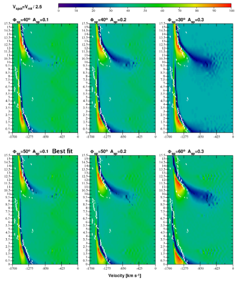
Figure 12 shows part of an atlas of one-spot models. The Figure shows six dynamic spectra computed with Wind3D which are closest to the best-fit solution. The Figure contains certain combinations for spot parameters =0.1, 0.2, & 0.3, and =30°, 40°, 50°, & 60°.
We first discuss the goodness of fit by considering how well the position of the model flux minima match the observations. The computed spectra are shown between 0 and 1700 , with the underlying smooth P Cygni wind profile subtracted. The computed flux minima in the DAC are marked with black dots, while the flux minima of the observed DAC are over-plotted with white dots. We vary the spot parameters and until a best match between the black and white dots is obtained. When we increase from 0.1, and 0.2, to 0.3 in the upper panels of Fig. 12, the base of the DAC extends toward velocities redward of 1000 that are not observed in HD 64760 (Sect. 3). We therefore find that does not significantly exceed 0.1. For 0.05, the morphology of the computed DAC compares very well to the observed DAC, and can be determined from a best fit to the detailed velocity position of the DAC flux minima over time. We apply a least-squares minimization method to the observed and computed DAC flux minima (black and white dots) yielding a best fit for models with between 40° and 50°. When =60° (lower right-hand panel) the computed DAC base crosses the observed DAC base too rapidly. If is lowered to 50° (at most) the velocity positions of the flux minima at the DAC base shift bluewards almost linearly over time (lower left-hand panel) conform with the observed DAC evolution. For 0.1 and 40° the DAC becomes invisible against the underlying smooth wind absorption. Our best-fit solution with a one-spot model is therefore: = / 2.5; and = °.
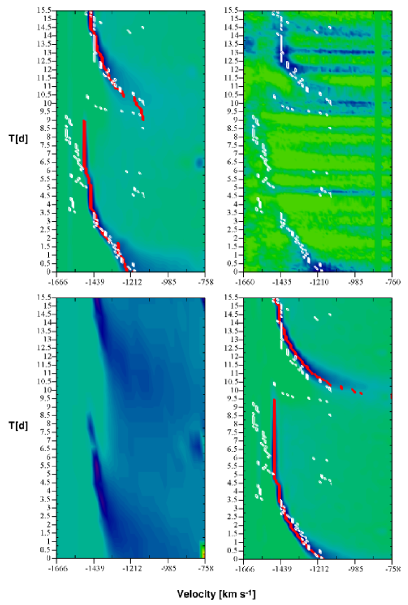
Figure 13 compares the best fit dynamic spectrum (upper left-hand panel) with the observed spectrum (upper right-hand panel). The computed dynamic spectrum correctly fits the observed flux difference spectrum in great detail. The velocity positions of the flux minima in the computed DAC (marked with red dots) differ by less than 50 from the observed velocity positions (white dots) for between 0 and 3.5 d (lower DAC), and for between 10 and 15.5 d (upper DAC). Over these time intervals the computed flux evolution in the DAC base correctly fits the detailed shape and morphology changes of the observed spectra.
We proceed with a detailed comparison of the observed DAC shape and the models. In Fig. 14 we compare the computed (left-hand panel) and observed (right-hand panel) shape and morphology at the DAC base for 0 d 3.75 d. The dynamic spectra are plotted between 758 and 1666 , revealing the slanted triangular shape of the DAC base. The characteristic shape results from wind regions within a few above the stellar surface where the density increase of the CIR spreads out above the spot. The DAC line formation region rotates in front of the stellar disk and samples a decreasing range of (projected) radial wind velocities along the line of sight causing a narrower DAC base over time. The FWHM of the computed DAC decreases from 100 at =0 d to 20 around =3.5 d, consistent with the observed DAC narrowing. The DAC width is small and stays nearly constant over the next 6.5 d, after which it fades away. The ‘tube-like’ extension of the DAC base also corresponds to the observations (upper right-hand panel of Fig. 13). It results from the CIR above 20 in the DAC line formation region where the wind velocity is within 5% of =1500 . The DAC samples only a very small range of wind velocities around , although its formation region (in front of the disk) extends geometrically from 20 to 30 . The DAC approaches , remains very narrow and visible, until the outer wind regions in the CIR rotate out of the observer’s line of sight. The time scale over which the DAC remains visible is set by the curvature of the CIR around the star which mainly depends on . Note that the computed DAC fades away after 10 d in the best fit model, as is observed in HD 64760. However, the velocity positions of the tube-like DAC feature observed between = 7 and 10 d somewhat exceed the DAC velocities of our best fit model by 100-150 . The smooth wind model has =1500 , which we slightly vary to improve the fit. We find however that changing by 200 leaves the spot parameters practically unchanged since the best fit criterion primarily relies on the DAC shape and morphology between =0 d and 7 d.
5.2 Two-spot model fits
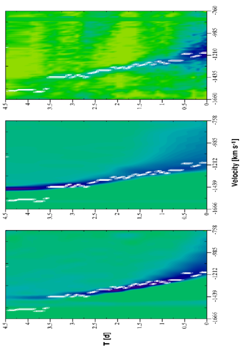
The upper left-hand panel of Fig. 13 shows the best fit for a two-spot model with = / 5. Models with two unequal spots better match the detailed DAC shape compared to our one-spot model fits. The spot parameters are varied separately until the best fit to the detailed shape and morphology of the observed upper and lower DAC (upper right-hand panel) is accomplished. We find the best fit to the lower DAC with a spot of and = °. The upper DAC is best fit with a second spot inserted on the opposite side of the stellar equator with and = °. Since the spot velocity is halved compared to one-spot models, the curvature of both CIR wind structures in Fig. 7 diminishes, yielding DAC shapes that are less curved. The left-hand and middle panels of Fig. 14 show the best fit to the detailed shape of the lower DAC with one- and two-spot models. The best two-spot fit to the lower DAC is an improvement and the computed flux minima correctly match the almost constant drift observed for its flux minima over time. The shape of the upper DAC flux minima is somewhat more curved (but less sharply defined due to the intersecting modulations), while its base is slightly more blue-shifted compared to the lower DAC. The upper DAC is therefore best fit using a somewhat larger = 30°. The larger spot opening angle used for the upper DAC broadens the computed width at its base and shifts the velocity positions of the flux minima very close to the observed values. The velocity extension of the upper DAC base somewhat decreases by reducing to 0.08 compared to the lower DAC (see also Sect. 4.3.3). One-spot models with =/2.5 produce DACs that accelerate considerably faster than a two-spot model with the same spot parameters, but having =/5. On the other hand, if the is also set identical for one- and two-spot models the differences in DAC shapes are very small and solely result from weak hydrodynamic interactions between the CIRs in the two-spot model (in the CIR tails at large wind velocity).
We also computed models with four and eight spots inserted at equal distances around the stellar equator. For models with four spots we set = / 10, with - and -values for all four spots comparable to the two-spot best fit model parameters (lower left-hand panel of Fig. 13). We find however that hydrodynamic interactions between the four CIRs become stronger and substantially alter the resulting DAC structures. The high-velocity tail of the CIRs can partially overlap with the structures at the base of the wind from the trailing CIRs. The base of the upper DAC therefore time overlaps too long with the high-velocity tube-like extension observed in the lower DAC. The detailed morphologies of DACs computed with four- and eight-spot models are not sufficiently well separated over time to be compatible with the behavior of the DACs observed in HD 64760.
The best fit models are obtained from a least-squares fit to the minima of the lower DAC for a grid of one-spot models and a grid of two-spot models separately. The least-squares fits to the lower DAC uses 36 spectra observed between 0 and 3.5 d because its DAC minima are poorly determined after 3.5 d (see Fig. 14). The least-squares fit procedure within both grids provides values that are significant indicators of the best fit spot parameters for the one-spot models or two-spot models. A least-squares fit comparison between one-spot and two-spot fits however is cumbersome strictly quantitatively because two-spot models always introduce two extra (spot) parameters in the fit compared to one-spot models. We compute a sigma (square root of the weighted sum of squares of velocity differences between the computed and observed DAC minima) of 22.2 for the best fit two-spot model, and 24.7 for the best fit one-spot model. These values are limited to 36 spectra between 0 and 3.5 d, and can therefore be compared. The two-spot best fit model quantitatively better fits the observed minima than the one-spot best fit model. The difference of 2.5 between these sigma values is however too small to conclude that the two-spot model significantly (in a statistical sense) better fits than the one-spot model when limited to the lower DAC. If the minima of the upper DAC are also included in the comparison, the difference of sigma values substantially increases, but the direct comparison of these values is more complicated because of the different number of free parameters.
We note however that none of the one-spot models yield the very linear shape we observe for the lower DAC. The one-spot models accelerate too fast, or the DACs are always too curved below the observed (rather straight) DAC shape. The two-spot models rotate twice slower and do provide this very linear DAC shape. The difference of DAC shapes in Fig. 14 is an improvement of the best fit with one-spot models. We also find that the two-spot best fit model yields a substantial broadening of the long-wavelength wing of the lower DAC base (between 0 and 1 d), which better than the one-spot best fit model corresponds to the width changes observed in the lower DAC. It results from the smaller spot velocity in two-spot models. The long-wavelength DAC base wing further broadens in the four-spot models (Fig. 13) which rotate another factor of two slower. One-spot models leave no room to adjust for the observed shape of the upper DAC which is visibly (although perturbed) slightly different from the lower DAC. For example, in the lower right-hand panel of Fig. 13 the best fit one-spot model yields computed DAC minima that fall below the lower DAC and above the upper DAC. This fit problem is removed with the best fit two-spot model (upper left-hand panel).
Our best fit procedure does not include the detailed evolution of the DAC depth because the current hydrodynamics does not compute the extension of the models above and below the equatorial plane. The computed DAC depth is therefore determined by the geometric height of the CIR which we set to 0.5 above and below the equatorial plane. An increase of of the structured wind model enhances the DAC depth in the P Cygni absorption profile because the amount of scattering due to the CIR in front of the stellar disk enlarges. We assume that the CIR height remains constant with distance from the star, having a fixed geometric height of 0.5 (the latter value is very close to the maximum height of a circular spot extending over 25° above and below the equatorial plane we find for a best fit with one-spot models). The relative variation of the DAC depth over time is however dependent on the assumption of a fixed geometric height for the CIR model. The actual CIR height is of course expected to also increase with distance from the stellar surface (e.g. due to the 1/ decrease of the smooth wind density), causing the large-scale wind structures to grow in latitude over a ‘flaring angle’ from the star. We however checked with 3D transfer calculations that and the flaring angle do not influence the detailed DAC shape or morphology we use for our best fits. In principle and the flaring angle can be determined from fully 3D hydrodynamic model calculations. They would allow us to also invoke the detailed DAC depth changes in our best fit procedure. A calculation of more sophisticated 3D models is however beyond the scope of this paper. The DAC shape and morphology suffice to obtain the best spot parameters for large-scale equatorial wind structures.
While we assume in this paper that sin for HD 64760, the inclination angle could be considered as an additional free parameter in the 3D radiative transfer computations. The detailed model geometry ( and flaring angle) of the structured wind influences the column densities that result from the CIRs along the line of sight for an observer slightly above or below the equatorial plane. Small flaring angles decrease the relative DAC depth formed at the base of the wind (at small velocities in the dynamic spectra), while large inclination angles decrease the relative DAC depth formed in the outermost wind regions (at large velocities). Important influences of the observer inclination angle on the dynamic spectra are shown in the left-hand panel of Fig. 14 with =85°. Around = 3 d the DAC depth decreases rapidly because the CIR in wind regions above 10 is tilted below the stellar disk when viewed by the observer above the plane of the equator (compare to the lower right-hand panel of Fig. 13 with =90°). A larger decrease of decreases the DAC depth further. The DAC becomes invisible for 80° when is constant and set equal to 0.5 in our 3D radiative transfer calculations. These calculations reveal that the observer line of sight towards HD 64760 does not exceed 10° from its equator-on direction, or that sin 0.984.
6 Discussion
6.1 Additional Mass Loss Rate
At first sight, it may seem that we do not have enough information to evaluate the mass-loss rate of the structured wind models because the hydrodynamics equations are solved in the equatorial plane only. However, we do assume that the spots are circularly symmetric on the stellar surface, which we can use to determine the mass-loss rate. To first approximation, we can assume that very close to the stellar surface the wind density and radial flow velocity have the same circular symmetry as the spot. Hence, the mass-loss rate of the structured wind () for a one-spot model is:
| (2) |
where is the angle measured from the spot center. Transforming to standard spherical coordinates gives , where is the coordinate of the spot center. The assumption of circular symmetry in the wind is not exactly correct however, not even close to the stellar surface. The leading edge of the density spiral slows down due to collision with the smooth wind, which results in a decrease of the mass-loss rate at the leading edge close to the surface. (Note that the boundary conditions in the spot do not specify a mass-loss rate, but rather use a constant-slope extrapolation for the radial velocity and a fixed base density – see Cranmer & Owocki, 1996). To obtain a reliable estimate of the mass-loss rate, we therefore neglect this effect by replacing the values of smaller than the smooth wind -values with the smooth wind values.
We use this method to compute the effect of the CIR on the mass-loss rate. In Fig. 15 we plot as a function of spot strength and spot angle for a number of one-spot hydrodynamic models. The Figure clearly shows that the extra mass-loss rate due to the CIR is always very small. Our best-fit model with one spot in Sect. 5.1 yields an increase of only 0.6 % for the mass-loss rate.
The model mass-loss rates can be checked against a simplified version of Eq. (2). In the model, the additional line force due to the spot is only calculated for a position directly above the spot center, while for other positions we relate it to that directly above the spot center by using a Gaussian function of azimuthal angle (Sect. 2.3). If we simplify this by using a function that is unity above the spot and vanishes outside it, we find for a one-spot model :
| (3) |
where is the mass-loss rate over the spot. We can further use the approximate relationship between mass-loss rate and luminosity (), which casts Eq. (3) into:
| (4) |
We find very good agreement between the mass-loss rates derived from detailed hydrodynamic models with Eq. (2) and the approximation of Eq. (4). This demonstrates that our method of computing the mass-loss rates for structured wind models is appropriate.
Equation (4) can be extended to include two symmetrical spots:
| (5) |
Applying a similar formula to our best-fit model with two asymmetrical spots (Sect. 5.2), we find a mass-loss rate increase of only 0.5 %.
Only a relatively small enhancement of the mass-loss rate in the smooth wind is required to maintain the large-scale density- and velocity-structures in the equatorial plane of radiatively accelerated hot star winds. Figure 16 shows the density contrast / along the CIR in the best-fit one and two-spot hydrodynamic models of HD 64760. The density enhancement in the CIR compared to the smooth wind density is only 32% at most (for the two-spot model). This type of large-scale wind structure does not reveal the dynamic flow properties of a shock wave, but rather of a rotating density wave. The small density increase in the CIR signals that these large-scale extended wind structures can also easily be perturbed by other types of dynamic wind structures that may exist on smaller length scales in winds of massive hot stars. The best example would be the structure due to the instability of the radiative driving mechanism (Owocki et al., 1988). The presence of DACs therefore provides a substantial constraint on the amount of clumping present in the wind: too much clumping would destroy the DACs (Owocki, 1998). The large-scale wind structures are a direct consequence of local irregularities in the radiative driving source at the base of the wind that involve limited variations of the surface intensity caused by dynamic surface structures that trail the stellar rotation.
6.2 Comparison with Previous Work
Kaufer et al. (2006) studied the observed photospheric and H line profile variations of HD 64760. In the photospheric lines they detected non-radial pulsations (NRPs) with three closely spaced periods ( h, h, h, in order of decreasing amplitude). To explain the variability in the H line, they proposed a model in which the beat period between and ( d) is responsible for the CIRs in the wind. Both periods have quantum numbers and , so there are two diametrically opposed spots on the equator. In general, the interference between modes with arbitrary quantum numbers can result in considerably more complicated interference patterns than is the case here. Because , the beat pattern moves in the opposite direction of rotation, with . The whole pattern therefore rotates in d. Because there are two spots, the effects on H repeat with the beat period of 6.8 d.
A literal application of the Kaufer et al. (2006) model to the IUE data does not work, because the timescale over which their model repeats (6.8 d) is not compatible with the observed 10.3 d timescale in the UV DACs. This is the main reason why we did not use the specific values from the Kaufer et al. (2006) work, but only their important idea of using spots that need not rotate with the rotational velocity.
Nevertheless, it should be noted that the beat period calculated by Kaufer et al. (2006) is quite sensitive to the accuracy with which the NRP periods have been determined. A change in periods and of only 0.0235 h would result in a 10.3 d beat period, rather than a 6.8 d one. From the power spectrum presented in their Fig. 5, it is clear that the NRP periods are not determined to such a precision. We also note that their 6.8 d period is not compatible with the suggested 2.4 d period in H. Interference between periods and can give a 2.4 d beat period, provided that small shifts to both periods are applied. It is therefore conceivable that the UV DACs are due to a beat pattern between and , while the variability in H and the UV modulations are due to a beat pattern between and . It of course remains to be explained why the - beat pattern is only seen in the UV DACs and the - one only in Halpha. The critical test is to calculate both the Si iv and the H line profile variations with our code. We defer this to a subsequent paper.
7 Summary and Conclusions
In this paper we show that a combination of advanced hydrodynamic and radiation transport calculations in three dimensions can correctly fit the detailed behavior of Discrete Absorption Components observed in variable UV wind lines of the hot supergiant HD 64760 (B0.5 Ib). The best fits are accomplished with sophisticated numerical simulations that invoke the physics of the transport of radiation in fast accelerating stellar winds. The hydrodynamic models use spots of enhanced brightness on the stellar surface to initiate large-scale density- and velocity-structures rotating in the plane of the equator.
We confirm and somewhat refine the conclusions of Cranmer & Owocki (1996) regarding the effects of spot strength and opening angle on the resulting CIRs. We also confirm their result that DACs are mainly formed in the velocity plateau between the kink and the CIR. In some cases, however, the density enhancement is responsible for the DAC formation (e.g. at low velocities). The conclusion of Hamann et al. (2001) that (for spots locked onto the stellar surface) the DAC acceleration does not depend at all on the stellar rotation rate, cannot be extended. This is mainly due to the effect of the centrifugal acceleration, which already plays a role for the underlying smooth wind structure. Even when artificially changing the CAK parameters to compensate for this, a (small) effect would remain in the CIRs.
We find that the CIRs in fast-rotating HD 64760 are very extended density waves. The discrepancy between the 10.3 d recurrence time of the DACs and the estimated 4.12 d rotation period is direct evidence that spots cannot rotate with the stellar surface. For a two-spot model, they instead lag 5 times (i.e. 2 10.3 / 4.12) behind the stellar surface rotation. The best fits to the observed DAC shape and morphology show that the Co-rotating Interaction Regions are caused by bright spots at the base of the wind that do not exceed the surface brightness by more than 205%. The opening angles of the (circular) spots are around 20° and 30° diameter, hence together covering an appreciable fraction of the stellar surface area. The structured wind models reveal density enhancements that do not exceed the density of the surrounding smooth wind by more than 30 %. The wind flow radially crosses the CIRs in the plane of the equator where it decelerates by less than 140 . The base of the DACs form in wind regions within a few above the surface where extra material spreads out above the spots. The width of the DACs decrease over time because the CIR structures rotate across the stellar disk, causing regions of larger optical depth farther out in the accelerating wind where the radial velocity dispersion in front of the stellar disk decreases. The properties (shape and dynamics) of the DAC line formation regions are uniquely determined by the spot properties at the base of the wind. It enables us to obtain a unique best fit to the shape and morphology of the DACs. We find a better fit to the shape of the upper and lower DACs with a two-spot model than with a one-spot model. Our detailed transfer calculations correctly match the (slanted) triangular shape of the DAC base that further extends into a (tube-like) bluewards-drifting narrow absorption feature observed in HD 64760 (and also in Per). The spots at the surface increase the total mass-loss rate of the smooth symmetric wind model for HD 64760 by only 0.5%.
We conclude that the large-scale structured wind of HD 64760 is caused by perturbations of the surface intensity that trail the fast surface rotation. This points to dynamic structures at the base of the wind that do not co-rotate with the stellar surface (unlike, e.g., surface magnetic fields). Such structures could possibly result from an interference of non-radial pulsations traveling the stellar circumference with periods set by the properties of permitted stellar pulsation modes. The relatively small perturbations that are required to create these DACs probably explains why they are so ubiquitous. Their presence also puts a substantial constraint on the amount of clumping that can be present in the wind. The large-scale coherent CIR structures may become perturbed by wind clumping on much smaller length scales. They will however built up again very rapidly as well, provided that the perturbation time-scales are sufficiently short for the CIR structures to completely develop and to cause the UV DACs. In future work we will investigate the effect of CIRs on other spectral lines and other stars, trying to best fit the observational data. For stars not observed close to equator-on, we will develop 3D hydrodynamic models.
APPENDIX
Appendix A 3D Transfer Formalism and Discretization
We denote by the vector the direction in which the light rays travel at position coordinates . =(,) denotes the specific intensity at frequency of radiation traveling in direction through point (or the direction of photon extinction at ). We solve the transfer problem in the observer frame because the co-moving frame formulation is not applicable to structured winds that can expand asymmetrically and that have non-monotonic wind velocity structures. When we denote the opacity and emissivity of the material =(,) and =(,), respectively, the time-independent monochromatic transfer equation at for a ray traveling in direction is . = . We use the two-level atom approximation with complete frequency redistribution so that = (1-) + , where = () is the line source function, = (,) the Planck function at , the ‘thermalization parameter’ in the non-LTE transfer problem, and the frequency-weighted mean intensity at . In this paper we solve the pure scattering problem for resonance lines formed in the very extended winds of massive stars that are considered to be isothermal in the lines formation region. In these conditions the spontaneous de-excitation rate greatly exceeds the collisional transition rate. We therefore assume = 0, and currently neglect LTE contributions in the transfer problem. It permits to solve the pure scattering transfer equation with the line source function at
| (A1) |
which integrates the specific intensity over all spatial angles , weighted by the line profile function . and denote the two spherical coordinate angles with =sin() . Note that we use instead of the more common , to avoid confusion with the profile function. When we denote the rest frequency of the line and the wind velocity vector at , the Gaussian line profile function = is
| (A2) |
denotes the line width = /c, with the mean thermal particle velocity and the turbulence velocity. We assume a Gaussian profile function for lines that are not intensity saturated. We do not consider line formation on the root part of the curve of growth, which would otherwise require parameterized damping profile functions. Also, we currently do not include a partial redistribution or correlation function in the atom’s frame because the 3D transfer problem should remain tractable by assuming complete redistribution over all line frequencies. Note that the integration of Eq. (A1) yields a frequency independent line source function in , which renders the problem of lambda iteration on independent of detailed frequency redistribution in the line profile.
The 3D scattering transfer problem consists of calculating by summing in Eq. (A1) over contributions from light rays that travel through from all directions, while accounting for Doppler effects in Eq. (A2) caused by the local wind velocity , and lambda iterating till becomes consistent with the radiative transfer equation. With = and = the isotropic contributions from the continuum radiation, and anisotropic contributions from the line radiation to and , the transport equation for stationary advection of the radiation field with respect to is
| (A3) |
where =() denotes the continuum source function and =/.
The time-independent multi-dimensional radiative transfer problem involves the development of a sophisticated numerical scheme that has to be tailored to solve a Boltzmann equation for photons. A wide variety of such algorithms is discussed in the literature which, dependent on the considered astrophysical conditions, are suitable to solve this equation from its diffusion limit (optically thick) to the pure transport (optically thin) limit. In astrophysical line and continuum transport, where scattering cannot be neglected, one applies a finite element discretization technique to solve an integro-differential equation (or a set of them). Generally, the complexity of this transfer problem results from the fact that due to scattering the radiation field is not only determined by local gas conditions but has to be consistent with the (atomic) state of the matter through which it can propagate over large geometric distances. While for 1D problems numerical methods are well established (e.g., Hubeny, 1997), adequate solutions for 3D problems are still in their infancy. A concise overview of 3D non-LTE radiative transfer problems in the past decades has recently been presented in Hauschildt & Baron (2006). We opted to implement Adam’s (Adam, 1990) spatially implicit first order method because it is one of the few 3D schemes that has successfully been applied to spectral lines that form in astrophysical conditions such as Be-star disk winds (e.g., Hummel, 1994).
Adam’s method consists of integrating Eq. (A3) for a finite volume in a Cartesian system of coordinates. The computation of and involves solving a system of integro-differential equations (Eqns. (A1) & (A3)) for which we consider an equidistant 3D rectangular grid with grid-points ==(,,) where =1.., =1.., =1.., and with velocity vectors = =(,,). Along a chosen direction , Eqn. (A3) can be discretized in the observer frame, and cast into
| (A4) |
The monochromatic specific intensity =) in is computed with Eq. (A4) by incrementing , , and by or depending on the direction of the rays in the grid. A general application of the Adam’s method treats as a parameter, while it set equal to throughout. Since is constant in an isothermal wind over one line width, we can set equal to a constant value. The detailed treatment of continuum processes is not included at this point. For our application of Adam’s method in this paper, we set =0 and =0 throughout the wind, and only use non-zero values for the continuum flux emitted at the stellar surface. We set the boundary conditions =0 and =0 for grid-points outside the grid. To be consistent with the nearly spherical geometry of a stellar wind, we also set these boundary conditions on the sphere that just fits inside our simulation volume. The corners of the grid ( ) therefore also have =0 and =0. At the boundary of the grid we set =0 and solve Eq. (A4) by stepping through the indices i,j,k. This is done for a set of observer frequencies and a number of directions specified by angles (,). We then compute or =() with a quadrature sum over ;
| (A5) |
The summation in Eq. (A5) can be limited to an interval (1..) around the rest frequency that covers the entire wind line (i.e. with a P Cygni profile). The summation over angular coordinates (,) is computed with a number of integration points that decreases toward higher latitudes on the sphere by using =() sin(). The calculation of therefore sums angles (or directions ) that are isotropically distributed around . It ensures that the 3D transfer is correctly solved for random opacity and velocity distributions (i.e. no preferential directions are considered for transfer in for example an equatorial disk). Note in Eq. (A1) that both and are direction dependent which makes the accuracy of Eq. (A5) very sensitive to the total number of directions in the summation. The number of (or ,) in Eq. (A5) scales with the size of the grid (,,), because grid-points at increasing distances from require finer sampling of to ensure the same accuracy of . The quadrature coefficients , , and in Eq. (A5) are computed with the fast (and simple) three-point Simpson formula for uneven grid-sizes, while Simpson’s 3/8 rule is used in case of even grid-sizes.
Equations (A4) and (A5) are solved iteratively whereby converges to a solution that changes by less than 1% over following cycles (exact lambda iteration). This technique is used to evaluate over successive iterations (iteration between radiation transfer and statistical equilibrium), followed by one final transfer iteration that computes the emergent line fluxes for a given set of directions . For the implementation of Wind3D the transfer computations are separated into an ‘iteration phase’ (discussed in Appendix B) and an ‘interpolation phase’ (Appendix C) because of memory limitation requirements and parallelization optimizations.
Appendix B 3D Lambda Iteration
During the iteration phase Wind3D computes the lambda iteration on in every grid-point starting from initial values that are well chosen as to limit the number of lambda iterations. The starting values are computed with the Sobolev approximation in Eq. (A4). The structured wind opacity in strong UV wind lines is computed from the wind density contrast since /, where is the frequency integrated line opacity (i.e. = ) The smooth wind opacity in the lines is given by the Groenewegen & Lamers (1989) parameterization:
| (B1) | |||||
| (B2) |
where is the parameter of a velocity law for the surrounding smooth wind. is the radial wind velocity in , and the thermal broadening for the scattering ion. Note that this neglects the large turbulent broadening found by Hamann (1981) and Groenewegen & Lamers (1989). , and are the opacity parameters, and the other symbols have their usual meaning. These opacity parameters determine whether or not the absorption portion of the computed profile intensity saturates. The values of the parameters are determined from an approximate fit of the computed average flux profile to the observed line profile. The detailed shape of the computed underlying line profile is not further optimized as we do not model the precise DAC depth in the profile, but rather its shape and FWHM evolution. The value of in Eqns. (B1) and (B2) is however determined from a best fit using a -velocity law to the smooth wind structure of the hydrodynamic model. For our best fit hydro model of HD 64760 we find .
It is of note that Adam’s scheme uses the widespread short characteristics method (e.g., Koesterke et al., 2002). The method is rather straightforward to implement for solving the non-relativistic, two-level atom, 3D transfer problem with complete frequency redistribution, which includes the solid angle and frequency grid parallelization. We find that this is particularly the case for the pure scattering problem in optically thin (wind) line formation conditions we consider in this paper. Adam’s method of lambda iterating the line source function to consistency with the transfer equation in a two-level atom proves to be very efficient and avoids the usual problems with non-convergence. For the pure scattering problem (=0) Wind3D always converges within a dozen iterations at most. Adam (1990) already pointed out that the method of Cartesian upwind discretization is unconditionally stable because only positive terms occur in Eq. (A4) (see also the study by Hummel (1992) of the transfer scheme). Our combination of a starting Sobolev source function with Adam’s discretization method provides an adequate lambda iteration scheme that is particularly suited for 3D scattering dominated transfer in asymmetric wind opacity- and velocity-structures.
The short characteristics method is however known to suffer from beam widening because the interpolation introduces angular diffusion in the numerical solution. The long characteristics method removes this defocusing problem because much higher accuracies can be achieved with it. The latter method is however computationally very expensive if one wants to sample high angular resolution, so as to accurately sample space at large distances from the source in an extended structured wind. It is also time-consuming because the long characteristics usually cover the same part of the transfer domain many times, which introduces strong redundancy. Long characteristics methods have only recently been examined within the framework of 3D radiative line transfer, but still await applications to real astrophysical problems (Baron & Hauschildt, 2007).
In our current implementation, Adam’s method also requires large memory storage capacity during the iterations because the computation of in Eq. (A4) requires to store two matrices for of at least elements for lightrays traveling in the forward and backward (incrementing with 1 and 1) direction along the -axis of the grid. This number has to be multiplied by the number of directions that is considered for the isotropic integration of in Eq. (A5) and the frequency resolution of the line profile, yielding 2 matrix elements per iteration cycle. The requirement that the integration accuracy of is maintained toward larger grid-sizes demands that the number of directions scales linearly with . For we therefore find that the required memory capacity scales with for fast computation of . For example, a doubling of the size of a cubic grid requires an increase of total memory with at least a factor of 32. In principle the large memory requirements can be reduced by solving Eq. (A4) monochromatically in one direction (per and per ) whereby Eq. (A5) is then computed in incrementing steps. The bottleneck of the 3D lambda iteration is however in Eq. (A5), which can adequately be parallelized by distributing the frequencies (and directions) over different threads (multi-threading). Wind3D currently implements a parallelization strategy that provides fastest possible integration of . The parallelization technique of yields excellent load balancing results with the least occupied CPU (using one thread per CPU) always performing within a few percent of the most occupied one.
We also implemented 3D lambda iteration in Wind3D that invokes an accelerator scheme to improve convergency times for the source function calculation. We use a linear average of source functions computed over preceding iterations cycles to predict the source function for the next iteration. In case of slow convergence (e.g. at very large optical depths and 1) lambda acceleration can shorten iteration times with factors of 3 to 5. For the pure scattering case (=0) we however find that the lambda iteration can be converged within a limited number of iterations, which turn out hard to decrease further using the acceleration scheme. The combination of 3D source functions computed during n past iterations also requires to store n additional array elements. These large memory requirements are a setback of the acceleration scheme when convergence is already sufficiently fast.
When 0 1 however, one classically starts the source function iterations with (see Adam, 1990) or (Hubeny, 1997), but which are both useless in case =0. Towards very small values of increasingly more iteration steps are required (since 1/, e.g. Mihalas & Weibel-Mihalas, 1984), but which do not become unacceptably large as long as the initial source function values are well-chosen, i.e. by starting from an escape probability approximation for optically thin wind conditions. For the major portion of our 3D models information propagates nearly directly from the stellar surface to any point in the wind, because there is nearly no opacity between the emission of a photon at the stellar surface and its absorption in the wind. The thickness of the 3D structured wind models is limited to 1 around the equatorial plane. The majority of the 3D wind model is therefore a smooth -wind structure. Only the structured wind regions close to the surface (where the line optical depth increases) slow down the convergence rate. The initial source function values in 90% of the model are already very close to the final values, and only 10% of the model (around the plane of the equator) requires further iterations of to self-consistency.
Finally, 3D lambda iteration with Wind3D assumes symmetry about the plane of the equator of the central star. The code however accepts arbitrary 3D wind structures that are asymmetric about the equatorial plane. Wind3D first performs the lambda iteration for the northern hemisphere, followed by the southern hemisphere. It offers the advantage that iteration times become halved when equator-symmetric wind structures are (commonly) adopted. Our hydrodynamic wind models are symmetric about the plane of the equator so that the lambda iteration can be converged for the northern hemisphere, followed with a convergence test of the source function values in all grid-points of the southern hemisphere.
Appendix C 3D Radiative Transfer Solution
An important aspect of the 3D transfer problem is that the computation of the line source function consistent with the transfer equation through lambda iteration takes orders of magnitude more time than only solving the 3D transfer equation (with a fully iterated source function) to compute emergent line fluxes. This results from the time-consuming geometric and frequency integration in Eq. (A1) required to iterate at every grid-point, compared to the fast computation of the specific intensities with Eq. (A4) when and are available. The accuracy of the iterated line source function therefore directly determines the accuracy of line fluxes computed with the transfer equation. This interdependence is particularly important when computing small flux variations inside wind line profiles due to small changes of the line source function caused by local density- and velocity-structures in the stellar wind. In this paper we typically compute line flux variations of less than 100 wide in P Cygni profiles that can have total line widths of up to 5000 (from the blue edge velocity to the red velocity end of the emission lobe). Using about 100 frequency points is therefore sufficient to adequately sample the line profile for solving the transfer equation. On the other hand, the accuracy of in Eq. (A5) also strongly depends on the number of frequency points for integrating the profile function . But to resolve small flux variations in the absorption portion of the wind profile, the width of the line profile function has to remain sufficiently small as to not broaden them or render them invisible with respect to the overall flux profile of the line. When we adopt a FWHM of below 50 the frequency integration in Eq. (A5) samples the full width of line profile function at only three frequency points. An under-sampling of therefore limits the accuracy of and the resulting line source function. This problem cannot be resolved by only increasing the number of frequency points for the integration of because it linearly increases its computation time (per lambda iteration cycle) at the bottleneck of the 3D transfer problem. For the problem to remain tractable an increase of therefore requires to reduce the number of directions and to compute . An accurate integration of over a limited number of directions can hence only be accomplished when the number of grid-points is also limited.
We adopt an equidistant grid with ===71 for the calculation. The method we present is to linearly 3D interpolate the lambda-iterated line source function on a much finer grid with grid-points to solve the 3D transfer equation. Our method of 3D interpolating is very efficient and proves to be sufficiently accurate to resolve small high-frequency flux variations in broad P Cygni line profiles. The 3D interpolation procedure is permitted when the length scales of the local density- and velocity-structures in the wind are larger than the distance between the grid-points, or (, ) ( x, y, z). This condition applies to our hydrodynamic models we compute for the large-scale structures in winds of massive hot stars. Note that the 3D transfer equation (A4) has a term in which = contains the line profile function as well. Since we 3D interpolate on a finer grid the influence of the local velocity field on the emergent specific intensity is computed also more accurately because is directly dependent of (Eq. A2) through the Doppler effect.
Following Adam’s method for Cartesian grids, the monochromatic flux = can be computed by integrating over the three visible surfaces of the grid for any given direction determined by angles and ,
| (C1) |
In Eq. (C1) are the monochromatic intensities computed at the up- and down-side surfaces () of the block, are computed at the left- and right-side surfaces (), and at the front- and back-side surfaces (). Equation (C1) sums the intensities from the three surfaces that are visible from any direction (,), over projected surface elements with =/, =/, and =/. We also compute frequency integrated intensity images at the six surfaces of the grid with
| (C2) |
for six different combinations of perpendicular angles and , and where =(-)/ is the frequency resolution of the line profile. In this paper we apply Eq. (C1) for detailed 3D radiative transfer modeling of spectral lines formed in the tenuous and supersonic winds of massive hot stars. Applications of Eq. (C2) for 3D radiative transfer imaging will be presented elsewhere.
References
- Adam (1990) Adam, J. 1990, A&A, 240, 541
- Baron & Hauschildt (2007) Baron, E., & Hauschildt, P. H. 2007, A&A, 468, 255
- Bjorkman & Cassinelli (1993) Bjorkman, J. E., & Cassinelli, J. P. 1993, ApJ, 409, 429
- Blomme (1991) Blomme, R. 1991, A&A, 246, 199
- Brown et al. (2005) Brown, J.C., Barrett, R. K., Oskinova, L.M, Owocki, S.P., Hamann, W.-R., De Jong, J.A., Kaper L., & Henrichs, H.F. 2004, A&A, 413, 959
- Cranmer & Owocki (1996) Cranmer, S.R., & Owocki, S. P. 1996, ApJ, 462, 469
- De Jong et al. (2001) De Jong, J. A., Henrichs, H. F., Kaper, L., Nichols, J. S., Bjorkman, K., Bohlender, D. A., Cao, H., Gordon, K., et al. 2001, A&A, 368, 601
- Dessart (2004) Dessart, L. 2004, A&A, 423, 693
- Fullerton et al. (1997) Fullerton, A.W., Massa D. L., Prinja, R.K., Owocki, S. P., & Cranmer, S. R. 1997, A&A, 327, 699
- Fullerton et al. (2006) Fullerton, A. W., Massa, D. L., & Prinja, R. K. 2006, ApJ, 637, 1025
- Groenewegen & Lamers (1989) Groenewegen, M.A.T., & Lamers, H.J.G.L.M. 1989, A&AS, 79, 359
- Hamann (1981) Hamann, W.-R. 1981, A&A, 93, 353
- Hamann et al. (2001) Hamann, W.-R., Brown, J.C., Feldmeier, A., & Oskinova, L.M. 2001, A&A, 378, 946
- Hauschildt & Baron (2006) Hauschildt, P. H., & Baron, E. 2006, A&A, 451, 273
- Howarth et al. (1998) Howarth, I. D., Townsend, R. H. D., Clayton, M. J., Fullerton, A. W., Gies, D. R., Massa, D., Prinja, R. K, & Reid, A. H. N. 1998, MNRAS, 296, 949
- Hubeny (1997) Hubeny, I. 1997, in Stellar Atmospheres: Theory and Observations, eds. J.P. De Greve, R. Blomme, and H. Hensberge, Springer, Berlin
- Hummel (1992) Hummel, W., Ph.D. Thesis, Univ. of Bochum, 1992
- Hummel (1994) Hummel, W. 1994, A&A, 289, 458
- Kaper et al. (1999) Kaper, L., Henrichs, H. F., Nichols, J. S., & Telting, J. H. 1999, A&A, 244, 231
- Kaufer et al. (2006) Kaufer, A., Stahl, O., Prinja, R. K, & Witherick, D. 2006, A&A, 447, 325
- Koesterke et al. (2002) Koesterke, L., Hamann, W.-R., & Gräfener, G. 2002, A&A, 384, 562
- Krtička et al. (2004) Krtička, J., Barrett, R. K., Brown, J. C., & Owocki, S. P. 2004, A&A, 417, 1039
- Lamers et al. (1987) Lamers, H. J. G. L. M., Cerruti-Sola, M., & Perinotto, M. 1987, ApJ, 314, 726
- Lefever et al. (2007) Lefever, K., Puls, J., & Aerts, C. 2007, A&A, 463, 1093
- Massa et al. (1995a) Massa, D., Fullerton, A. W., Nichols, J. S., et al. 1995a, ApJ, 452, L53
- Massa et al. (1995b) Massa, D., Prinja, R. K., & Fullerton, A. W. 1995b, ApJ, 452, 842
- Mihalas & Weibel-Mihalas (1984) Mihalas, D., & Weibel-Mihalas, B. 1984, Foundations of Radiation Hydrodynamics, Dover Publ., New York
- Morel et al. (2004) Morel, T., Marchenko, S. V., Pati, A. K., et al. 2004, MNRAS, 351, 552
- Owocki (1998) Owocki, S.P. 1998, in Kaper L., Fullerton A.W., eds., in “Cyclical Variability in Stellar Winds”, ESO Astroph. Symp., Springer, Berlin, 325
- Owocki (1999) Owocki, S. P. 1999, Lecture Notes in Physics, 523, 294
- Owocki et al. (1988) Owocki, S. P., Castor, J. I., & Rybicki, G. B. 1988, ApJ, 335, 914
- Owocki et al. (1994) Owocki, S. P., Cranmer, S. R., & Fullerton, A.W. 1995, ApJ, 453, L37
- Owocki et al. (1996) Owocki, S. P., Cranmer, S. R., & Gayley, K. G. 1996, ApJ, 472, L115
- Owocki et al. (1999) Owocki, S. P., & Cohen, D. H. 1999, ApJ, 520, 833
- Prinja (1998) Prinja R.K., 1998, in Kaper L., Fullerton A.W., eds., in “Cyclical Variability in Stellar Winds”, ESO Astroph. Symp., Springer, Berlin, 92
- Prinja et al. (1995) Prinja, R. K., Massa, D., & Fullerton, A. W. 1995, ApJ, 452, L61
- Prinja et al. (2002) Prinja, R. K., Massa, D., & Fullerton, A. W. 2002, A&A, 388, 587
- Prinja et al. (2005) Prinja, R. K., Massa, D., & Searle, S. C. 2005 A&A, 430, L41
- Puls et al. (2006) Puls, J., Markova, N., Scuderi, S., et al. 2006, A&A454, 625
- Rybicki & Hummer (1978) Rybicki, G. B., & Hummer, D. G. 1978, ApJ, 219, 654
- Stone & Norman (1992) Stone, J. M., & Norman, M. L. 1992, ApJS, 80, 753
| Effective temperature | (K) | 24 600 |
| Luminosity | (L☉) | |
| Radius | (R☉) | 22 |
| Mass | (M☉) | 20 |
| Terminal velocity | (km s-1) | 1 500 |
| Mass loss rate | (M☉ yr-1) | |
| Projected rotational velocity | sin (km s-1) | 265 |
| Equatorial angular velocity | (s-1) | (sin = 1 assumed) |