Hyperbolic billiards with nearly flat
focusing boundaries. I

Abstract

The standard Wojtkowski–Markarian–Donnay–Bunimovich technique for the hyperbolicity of focusing or mixed billiards in the plane requires the diameter of a billiard table to be of the same order as the largest ray of curvature along the focusing boundary. This is due to the physical principle that is used in the proofs, the so-called defocusing mechanism of geometrical optics. In this paper we construct examples of hyperbolic billiards with a focusing boundary component of arbitrarily small curvature whose diameter is bounded by a constant independent of that curvature. Our proof employs a nonstardard cone bundle that does not solely use the familiar dispersing and defocusing mechanisms.

Mathematics Subject Classification: 37D50, 37D25, 37A25.

1 Introduction

Much has been written, in the scientific literature, about the hyperbolicity of billiards in two dimensions. So much that general principles have even been devised for the ‘design of billiards with nonvanishing Lyapunov exponents’. The expression is taken from the title of the 1986 seminal paper by Wojtkowski [W2], in which he beautifully links the question of exponential instability (i.e., positivity of a Lyapunov exponent) to a few simple observations from geometrical optics. By means of the powerful invariant cone technique [W1, K, CM], Wojtkowski gives sufficient conditions for a planar billiard to have nonzero Lyapunov exponents, this implying a fuller range of hyperbolic properties via the general results of Katok and Strelcyn on Pesin’s theory for dynamical systems with singularities [KS].

Wojtkowski’s conditions are rather undemanding for dispersing and semidispersing billiards (i.e., billiards in a domain $\Omega\subset\mathbb{R}^{2}$, a.k.a. table, whose boundary is the finite union of smooth convex pieces, when seen from inside $\Omega$), and much more restrictive for focusing, semifocusing and mixed billiards (that is, cases when $\partial\Omega$ is made up—completely or partially, respectively—by concave pieces). (Both in the dispersing and in the focusing case, the prefix semi- means that $\partial\Omega$ has some flat parts as well.) For the latter type of billiards, further work has been done by Markarian [M1, M2], Donnay [D] and Bunimovich [B3] (see [CM, Chap. 9] for an overview of the subject and [De] for an interesting variation).

If we call boundary component each smooth piece of $\partial\Omega$, one of the conditions in [W2] is that the inner semiosculating disc at any given point of a focusing boundary component must not intersect other components, or the semiosculating discs relative to other focusing components ([M1] has a similar condition). This is required in order to implement the so-called defocusing mechanism, which can be loosely described like this: One wants diverging beams of trajectories to keep diverging after every collision with the boundary. But at a focusing portion of the boundary a diverging beam may be bounced back as a converging beam. A solution around this problem is to let the converging beam travel untouched for a sufficienly long time until the trajectories focus among themselves and then start to diverge again.

The defocusing mechanism is the closest extension of Sinai’s original idea of extracting hyperbolicity from the expanding features of dispersing boundaries [S]. At least to our knowledge, it has remained unsurpassed since Bunimovich introduced it in 1974 [B1], to become very popular a few years later, when it was used to work out the famous stadium billiard [B2].

Sticking too much to the standard principles, however, creates a problem and somehow a paradox. The condition on the semiosculating discs, and each of its later analogues, requires a table with focusing components to have a diameter of the order of the largest radius of curvature among the focusing points of the boundary. To illustrate how this may seem a paradox, consider the following example: Take a unit square and replace three of its sides with circular arcs of curvature $k_{d}\in(-\sqrt{2},0)$ having their endpoints in the vertices of the square. In this paper we use the convention that the curvature is positive at focusing points of the boundary and negative at dispersing points, so the arcs are convex relative to the interior of the square; the condition $|k_{d}|<\sqrt{2}$ ensures that each pair of adjacent arcs intersects only at the common endpoint. The resulting billiard is semidispersing, thus belongs to the standard class and is well-know to be uniformly hyperbolic, Bernoulli, and so on [CM]. Now perturb the fourth side into a focusing circular arc of curvature $k_{f}\ll 1$. Now matter how small the perturbation, this new billiard will never satisfy Wojtkowski’s principle and is not currently known to be hyperbolic, although it presumably is.

This may not sound too strange. After all, certain perturbations of dispersing billiards are known to possess elliptic islands [RT, TR]. But the paradox is that the smaller the perturbation, the less adequate the standard technique; that is, the closer the billiard comes to be dispersing, the worse the method applies which is supposed to exploit the dispersing nature of the boundaries. Up until $k_{f}=0$, at which point everything suddenly, and abruptly, works again to the fullest power of the theory of hyperbolic billiards.

Here we address this problem and, although we cannot yet prove that the perturbed square billiard is hyperbolic, we devise a couple of models that make clear what the difficulties are in extending the current methodology. These billiards, which are modifications of the example just discussed, are depicted in Figs. 1 and 2. They are indeed two families of billiards, as we are interested in the case when the curvature of the focusing boundary goes to zero. We define an invariant cone bundle that exploits the fact that the focusing component is nearly flat, and thus almost always acts as a semidispersing boundary.

Figure 1: The main billiard table

In any event, we are able to answer the following questions in the affirmative:

1. Can one design a billiard whose hyperbolicity is proved via a set of invariant cones that does not use exclusively the dispersing/defocusing mechanism for beams of trajectories?

2. Can one construct a family of hyperbolic billiard tables with a (nonvanishing) focusing component whose maximum curvature approaches zero, and such that the area of the table is bounded above?

3. Can one require the diameter to be bounded above as well?

4. Are these billiards ergodic? (This will be proved in [BL].)

Figure 2: A modification of the main billiard table

Points 2 and 3 show, independently of the method utilized, that one can go beyond the apparent implication ‘almost flat focusing boundaries imply very large tables’.

This is the plan of the paper: In Section 2 we review the basic definitions of billiard dynamics. In Section 3 we present and adapt Wojtkowsky’s theory of invariant cones derived from geometrical optics. In Section 4 we define the first of our models and choose suitable cones to prove its hyperbolicity. In Section 5 we show that the billiard introduced before can be chosen with a bounded area, and finally we present a second model which has a bounded diameter as well.

Acknowledgments.  We would like to thank Gianluigi Del Magno for an instructive discussion on the subject. M.L. acknowledges partial support from NSF Grant DMS-0405439.

2 Preliminaries

A planar billiard is the dynamical system generated by the flow of a point particle that moves inertially inside a closed region $\Omega\subset\mathbb{R}^{2}$ and collides elastically at the boundary; the latter is assumed to have an infinite mass. This implies that the trajectory of the particle, near the collision point, verifies the well-known Fresnel law: the angle of incidence equals the angle of reflection. The region $\Omega$ is called the billiard table. We denote $\Gamma=\partial\Omega$ and assume that $\Gamma$ is piecewise smooth (at least $C^{3}$).

Let $(q(t),u(t))$ represent the position and the velocity of the particle at time $t$. It is an easy consequence of the conservation of energy that $\|u(t)\|=$ constant. Therefore, by a rescaling of time, one can always reconduct to the situation where $\|u\|=1$, which we assume throughout the paper. The product $\Omega\times S^{1}$ is the natural phase space of the billiard flow, with a couple of extra specifications: First, if $q\in\Gamma$ and $u$ points outwardly, then $(q,u)$ is identified with $(q,u^{\prime})$, where $u^{\prime}$ is the outgoing (i.e., inward) velocity of a collision at $q$ with incoming velocity $u$. Second, if $q$ is in a corner, the flow is not defined. The billiard flow preserves the Lebesgue measure on $\Omega\times S^{1}$, as it can be verified directly or by applying the Liouville Theorem to this nonsmooth Hamiltonian system.

Now let $\mathcal{M}\subset\Omega\times S^{1}$ be the set of all pairs $(q,u)$ with $q\in\Gamma$ and $u$ pointing inside the table. These pairs are sometimes called line elements [S] and $\mathcal{M}$ is evidently a global cross section for the flow. The corresponding Poincaré map $\mathcal{F}:\mathcal{M}\longrightarrow\mathcal{M}$ is called the billiard map and acts as follows: if $q^{\prime}\in\Gamma$ is the first collision point of the flow-trajectory with initial conditions $(q,u)$, and $u^{\prime}$ is the postcollisional velocity there, then $\mathcal{F}(q,u)=(q^{\prime},u^{\prime})$. $\mathcal{F}(q,u)$ is undefined when $q^{\prime}$ is a vertex of $\Gamma$, and is discontinuous at tangential collisions, i.e., when $u^{\prime}$ is tangent to $\Gamma$ in $q^{\prime}$. For the sake of simplicity, those latter line elements are removed as well from the domain of $\mathcal{F}$. The set of all removed $(q,u)$ is denoted $\mathcal{S}_{1}$, or $\mathcal{S}_{1}^{+}$.

We identify $\mathcal{M}$ with the rectangle $[0,L]\times[-\pi/2,\pi/2]$, where $L$ is the perimeter of $\Omega$: each $(q,u)$ is identified with the pair $(s,\alpha)$, where $s$ is the arclength coordinate of $q$ (relative to a fixed choice of the origin $s=0$ and oriented counterclockwise) and $\alpha$ is the angle (oriented clockwise) between $u$ and the inner normal to $\Gamma$ in $q$. The Lebesgue measure on $\Omega\times S^{1}$ induces an $\mathcal{F}$-invariant measure $\mu$ on $\mathcal{M}$ which, in the above coordinates, is described by $d\mu(s,\alpha)=c\,\cos\alpha\,dsd\alpha$. The constant $c$ is customarily chosen so that $\mu$ is a probability measure.

Let us indicate with $\mathcal{S}_{0}$ the set of all pairs $(s,\alpha)\in\mathcal{M}$ where $s$ corresponds to a vertex of $\Gamma$ or $\alpha=\pm\pi/2$. The set $\mathcal{S}_{1}=\mathcal{S}_{1}^{+}$ introduced earlier is morally given by “$\mathcal{S}_{1}^{+}:=\mathcal{F}^{-1}\mathcal{S}_{0}$”. For historical reasons, this is usually called the singularity set of $\mathcal{F}$, even though the differential of $\mathcal{F}$ is singular only at line elements resulting in tangential hits. Analogously, for $n>1$, $\mathcal{S}_{n}^{+}:=\mathcal{S}_{1}^{+}\cup\mathcal{F}^{-1}\mathcal{S}_{1}^{+}\cup\cdots\cup\mathcal{F}^{-n+1}\mathcal{S}_{1}^{+}$ is the set where $\mathcal{F}^{n}$ is not defined, which is called the singularity set of $\mathcal{F}^{n}$. We also introduce “$\mathcal{S}_{1}^{-}:=\mathcal{F}\mathcal{S}_{0}$” and, for $n>1$, $\mathcal{S}_{n}^{-}:=\mathcal{S}_{1}^{-}\cup\mathcal{F}\mathcal{S}_{1}^{-}\cup\cdots\cup\mathcal{F}^{n-1}\mathcal{S}_{1}^{-}$. These are the singularity sets for the powers of the inverse map $\mathcal{F}^{-1}$. Lastly, $\mathcal{S}_{\infty}^{+}:=\bigcup_{n=1}^{\infty}\mathcal{S}_{n}^{+}$, $\mathcal{S}_{\infty}^{-}:=\bigcup_{n=1}^{\infty}\mathcal{S}_{n}^{-}$, and $\mathcal{S}:=\mathcal{S}_{\infty}^{+}\cup\mathcal{S}_{\infty}^{-}$.

Each $\mathcal{S}_{n}^{\pm}$ is the union of smooth curves whose endpoints lie either on another such curve or on the generalized boundary of $\mathcal{M}=[0,L]\times[-\pi/2,\pi/2]$, which is defined as the boundary of $\mathcal{M}$ plus all the vertical segments $s=s_{i}$, where $s_{i}$ is the boundary coordinate of a vertex of $\Gamma$. If $L<\infty$, the number of vertices is finite, and the curvature of $\Omega$ is bounded, then $\mathcal{S}_{n}^{\pm}$ comprises only a finite number of smooth curves.

Under the above assumptions, $\mathcal{F}$ is a piecewise differentiable map with singularities, of the type studied by Katok and Strelcyn in [KS]. Among their results is a suitable version of the Oseledec Theorem which guarantees, for a.e. $(s,\alpha)=:x\in\mathcal{M}$:

1. A decomposition of the tangent space $T_{x}\mathcal{M}$ into $E_{x}^{+}\oplus E_{x}^{-}$. These one-dimensional spaces are dynamics-invariant in the sense that $(D\mathcal{F})_{x}E_{x}^{\pm}=E_{\mathcal{F}x}^{\pm}$, where $(D\mathcal{F})_{x}$ denotes the differential of $\mathcal{F}$ at $x$.

2. The existence of the Lyapunov exponents $\lambda_{\pm}(x)$, defined as

   $$\lambda_{\pm}(x):=\lim_{n\to+\infty}\frac{1}{n}\log\|(D\mathcal{F}^{n})_{x}v_{\pm}\|,$$ (2.1)

   with $v_{\pm}\in E_{x}^{\pm}$. Since $\mu$ is absolutely continuous w.r.t. the Lebesgue measure on $\mathcal{M}$, then $\lambda_{+}(x)=-\lambda_{-}(x)$. We adopt the convention that $\lambda_{+}(x)\geq 0$.

The dynamical system is hyperbolic, by definition, if $\lambda_{+}(x)>0$ almost everywhere. If the system is ergodic too, then $\lambda_{+}(x)=$ constant $=:\lambda_{+}$.

3 Geometrical optics and cone bundles

In this section, which liberally draws from [W2], we recall the basic tenets of the invariant cone technique for the hyperbolicity of planar billiards (cf. also [LW]), and prove a couple of results that are specifically designed for our systems.

Given $x\in\mathcal{M}$ and two linearly independent vectors $v_{1},v_{2}\in T_{x}\mathcal{M}$, we define the cone with boundaries $v_{1},v_{2}$ as the set

$$C(x):=\left\{av_{1}+bv_{2}\>\left|\>a,b\in\mathbb{R},\ ab\geq 0\right.\!\right\}.$$ (3.1)

If $C(x)$ is defined at every, or almost every, $x\in\mathcal{M}$ and the dependence on $x$ is measurable, we speak of $C\subset T\mathcal{M}$ as a measurable cone bundle.

A measurable cone bundle $C$ is said to be:

• invariant, if $(D\mathcal{F})_{x}C(x)\subseteq C(\mathcal{F}x)$ for $\mu$-a.e. $x$;

• strictly invariant, if $(D\mathcal{F})_{x}C(x)\subset C(\mathcal{F}x)$ for $\mu$-a.e. $x$;

• eventually strictly invariant, if it is invariant and, for $\mu$-a.e. $x$, there exists $n(x)\in\mathbb{Z}^{+}$ such that $(D\mathcal{F}^{n(x)})_{x}C(x)\subset C(\mathcal{F}^{n(x)}x)$.

The next theorem was proved in [W1].

Theorem 3.1

Given a billiard map $\mathcal{F}$ as described above, if there exists an eventually strictly invariant measurable cone bundle, then the Lyapunov exponent $\lambda_{+}(x)$ is positive for $\mu$-a.e. $x\in\mathcal{M}$.

In [W2] Wojtkowski reduces the invariance of a cone bundle to a problem of geometrical optics concerning the behavior of a family (a beam) of nearby trajectories. We present the main ideas.

To a tangent vector $v\in T_{x}\mathcal{M}$ in phase space is naturally associated a differentiable curve $\varphi:(-\varepsilon,\varepsilon)\longrightarrow\mathcal{M}$ such that $\varphi(0)=x$ and $\varphi^{\prime}(0)=v$. By construction, $\sigma\mapsto\varphi(\sigma)$ is uniquely determined in linear approximation around $0$. Using the representation of $\mathcal{M}$ as a subset of $\Omega\times S^{1}$, and the notation $\varphi(\sigma)=(q(\sigma),u(\sigma))\in\Omega\times S^{1}$, we construct the family of lines, or rays, $l^{+}(\sigma):=\left\{\left.\!q(\sigma)+ru(\sigma)\>\right|\>r\in\mathbb{R}\right\}$. Also, denoting by $u^{-}(\sigma)$ the outward-pointing, precollisional vector of $u(\sigma)$ at $q(\sigma)\in\Gamma$, we define $l^{-}(\sigma):=\left\{\left.\!q(\sigma)+ru^{-}(\sigma)\>\right|\>r\in\mathbb{R}\right\}$.

In first approximation, that is, when $\varepsilon\to 0^{+}$, the now infinitesimal beam of rays focuses in a point, which means that all rays, up to adjustments of order $\varepsilon$ in $(q(\sigma),u(\sigma))$, have a common intersection. We consider the case too where the common intersection is at infinity. This focal point is clearly a function of $v$ only: it is denoted $F^{+}(v)$ for the family $\{l^{+}(\sigma)\}$ and $F^{-}(v)$ for the family $\{l^{-}(\sigma)\}$. Let us call $f^{\pm}(v)$ the signed distances, along $l^{\pm}(0)$, between $F^{\pm}(v)$ and $q_{0}=q(0)$ ($l^{\pm}(\sigma)$ has the orientation induced by the parameter $r\in\mathbb{R}$, that is, outward for $l^{-}(\sigma)$ and inward for $l^{+}(\sigma)$, relative to $\Omega$). In the remainder, we will omit the dependence of $v$ from all the notation whenever there is no ambiguity. Indicated by $(ds,d\alpha)$ the components of $0\neq v\in T\mathcal{M}_{(s_{0},\alpha_{0})}$ in the natural basis $\{\partial/\partial s,\partial/\partial\alpha\}$, one has

$$f^{\pm}=\left\{\begin{array}[]{lll}\displaystyle\frac{\cos\alpha_{0}}{\pm k(s_{0})-\frac{d\alpha}{ds}},&&\mbox{if }ds\neq 0;\vspace{6pt}\\ 0,&&\mbox{if }ds=0.\end{array}\right.$$ (3.2)

Here $k(s)$ denotes the curvature of $\Gamma$ at the point of coordinate $s$ (as specified in the introduction, the curvature is taken positive at focusing points of the boundary, and negative at dispersing points). The formula (3.2) is derived, e.g., in [W2].

It is easy to see that $f^{\pm}$ are projective coordinates of $T_{x}\mathcal{M}$. Hence any cone of the type (3.1) can be described by a closed interval in the coordinate $f^{+}\in\overline{\mathbb{R}}$, where $\overline{\mathbb{R}}:=\mathbb{R}\cup\{\infty\}$ is the compactification of $\mathbb{R}$. Henceforth, for simplicity, we will drop the subscripts from the coordinates $(s_{0},\alpha_{0})$ of the collision pair. Also, we will use the imprecise terminology ‘the point $s\in\Gamma$’ to mean ‘the point in $\Gamma$ of coordinate $s$’. The next lemma is known in optics as the mirror equation [W2, CM].

Lemma 3.2

For an infinitesimal beam of trajectories colliding around the point $s\in\Gamma$ with reflection angles around $\alpha$,

$$-\frac{1}{f^{-}}+\frac{1}{f^{+}}=\frac{2k(s)}{\cos\alpha}.$$

We now present a visual description of the cone $C(x)=C(s,\alpha)$ on the configuration plane containing $\Omega$. For $s\in\Gamma$ and $\beta>0$, denote by $D_{\beta}(s)$ the closed disc of radius $1/|\beta k(s)|$ tangent to $\Gamma$ in $s$ on the internal side of $\Omega$. Analogously, for $\beta<0$, let $D_{\beta}(s)$ be the closed disc of radius $1/|\beta k(s)|$ tangent to $\Gamma$ in $s$ on the external side of $\Omega$. Consider also the two closed halfplanes delimited by $t(s)$, the tangent line to $\Gamma$ in $s$: let $D_{0+}(s)$ denote the internal halfplane, relative to $\Omega$, and $D_{0-}(s)$ the external one. See Fig. 3. The interior of $D_{\beta}(s)$ is indicated with $D_{\beta}^{\circ}(s)$.

Figure 3: The tangent line $t(s)$ and some discs $D_{\beta}(s)$. The yellow part of the trajectory is the locus of the focal points $F^{+}$ corresponding to a certain cone.

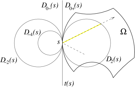
Lemma 3.3

Given a cone $C(s,\alpha)$ of the type (3.1), $v\in C(s,\alpha)$ corresponds to $F^{+}(v)\in l^{+}(0)\cap D$, where $D\subset\mathbb{R}^{2}$ is one of the following sets:

• $D=D_{\beta_{1}}(s)$;

• $D=D_{\beta_{1}}(s)\setminus D_{\beta_{2}}^{\circ}(s)$, with $|\beta_{1}|<|\beta_{2}|$;

• $D=D_{\beta_{1}}(s)\cup D_{\beta_{2}}(s)$, with $\beta_{1}\geq 0$ and $\beta_{2}\leq 0$;

• $D=\mathbb{R}^{2}\setminus(D_{\beta_{1}}^{\circ}(s)\cup D_{\beta_{2}}^{\circ}(s)\cup\{s\})$, with $\beta_{1}\geq 0$ and $\beta_{2}\leq 0$.

Moreover,

$$F^{+}(v)\in\partial D_{\beta}(s)\setminus\{s\}\quad\Longleftrightarrow\quad f^{+}(v)=\frac{2\cos\alpha}{\beta|k(s)|}.$$

Proof. By construction $F^{+}=F^{+}(v)\in l^{+}(0)$. Since $f^{+}$ is a coordinate on $l^{+}(0)$, a closed interval in the projectivized $f^{+}\in\overline{\mathbb{R}}$ corresponds, on $l^{+}(0)$, to either a closed segment or a closed halfline or the union of two disjoint closed halflines. Cases (a)-(d) cover all possibilities.

The second statement, for $\beta>0$, comes from elementary trigonometry (see Fig. 3), and it trivially extends to the case $\beta<0$ as well. Q.E.D.

The reason why, in Lemma 3.3, we chose such peculiar sets $D$ to cut a (projective) closed segment on $l^{+}(0)$, upon intersection, will be made clear by the next lemma. In particular, we will see that describing the cones in terms of the discs $D_{\beta}(s)$ will eliminate the dependence on $\alpha$ in the mirror equation of Lemma 3.2.

Lemma 3.4

For infinitesimal beam of trajectories colliding around $s\in\Gamma$, $F^{-}\in\partial D_{\beta}(s)$ if and only if $F^{+}\in\partial D_{\beta^{\prime}}(s)$, where

$$\beta^{\prime}=4\,\mathrm{sgn}(k(s))-\beta$$

(with the understanding that $F^{\pm}\in\partial D_{0\pm}$ means $F^{\pm}\in\{s,\infty\}$).

Proof. Let $\alpha$ be the angle of reflection (and thus of incidence) of the trajectory we are perturbing. Disregarding the case $F^{+}=F^{-}=s$, we know from Lemma 3.3 that $F^{+}\in\partial D_{\beta^{\prime}}(s)$ corresponds to $f^{+}=2\cos\alpha/(\beta^{\prime}|k(s)|)$. Also, $F^{-}\in\partial D_{\beta}(s)$ is equivalent to $f^{-}=-2\cos\alpha/(\beta|k(s)|)$ (the minus sign is needed because a focal point $F^{-}$ lying on the internal halfplane $D_{0+}(s)$ corresponds to a negative $f^{-}$ along $l^{-}(0)$, and viceversa). Direct substitution into Lemma 3.2 yields

$$\frac{\beta|k(s)|}{2\cos\alpha}+\frac{\beta^{\prime}|k(s)|}{2\cos\alpha}=\frac{2k(s)}{\cos\alpha},$$ (3.3)

whence the assertion. Q.E.D.

With the tools of Section 3, the problem of the cone invariance along a given trajectory can be reduced to the study of the focal points of one-parameter perturbations of that trajectory.

We single out the information that we need for our forthcoming proofs.

Proposition 3.5

For an infinitesimal beam of trajectories colliding around $s$ we have the following: If $s$ belongs to a focusing component of $\Gamma$, i.e., $k(s)>0$, then:

$$F^{\mp}\in D_{4}(s) \Longleftrightarrow F^{\pm}\in D_{0-}(s);$$

$$F^{\mp}\in D_{2}(s)\setminus D_{4}^{\circ}(s) \Longleftrightarrow F^{\pm}\in D_{0+}(s)\setminus D_{2}^{\circ}(s).$$

If $s$ belongs to a dispersing component of $\Gamma$, i.e., $k(s)<0$, then

$$F^{\mp}\in D_{-4}(s) \Longleftrightarrow F^{\pm}\in D_{0+}(s);$$

$$F^{\mp}\in D_{-2}(s)\setminus D_{-4}^{\circ}(s) \Longleftrightarrow F^{\pm}\in D_{0-}(s)\setminus D_{-2}^{\circ}(s).$$

Analogous equivalences hold for the interior of such cones. The situation is illustrated in Fig. 4.

Proof. We only prove the first statement, the other ones being completely analogous. Once again, we disregard the easy case $F^{+}=F^{-}=s$. We have $F^{-}\in D_{4}(s)$ $\Leftrightarrow$ $F^{-}\in\partial D_{\beta}(s)$, for $\beta\in[4,+\infty)$ $\Leftrightarrow$ (by Lemma 3.4) $F^{+}\in\partial D_{\beta^{\prime}}(s)$, for $\beta^{\prime}\in(-\infty,0]$ $\Leftrightarrow$ $F^{-}\in D_{0-}(s)$. Clearly, nothing changes if we swap $F^{-}$ and $F^{+}$. Q.E.D.

Figure 4: A geometric representation of Proposition 3.5. The left picture represents the first two statements (focusing border); the right picture represents the last two statements (dispersing border). Yellow/blue sets of focal points $F^{-}$ are mapped into yellow/blue sets of focal points $F^{+}$. The dependence on $s$ in the notation has been omitted.

4 Hyperbolicity

Fig. 5 shows the billiard table we are mainly interested in for the rest of the paper. We refer to it for the definition of the quantities $l,h>0$. The three dispersing components of the boundary $\Gamma$ are circular arcs of curvature $k_{d}\in(-\sqrt{2},0)$. Their union is denoted $\Gamma_{d}$. The focusing component is a circular arc of curvature $k_{f}>0$ and is denoted $\Gamma_{f}$. The remining, flat, part of the boundary is denoted $\Gamma_{s}$. The two rectangular portions of $\Omega$ which $\Gamma_{s}$ almost delimits will be referred to as the strips, or the corridors, or whatever one’s fancy suggests each time.

Figure 5: The definition of the table $\Omega$.

The geometric constants $l,h,k_{f},k_{d}$ are chosen via the following procedure. Keep in mind that we are interested in small values of $k_{f}$ (see the Introduction) and $h$ (see Section 5). One starts by fixing arbitrary values of $k_{d}$ and $h$. Then $k_{f}$ is determined by a geometric condition that we presently describe, with the help of Fig. 6. For $s^{\prime}\in\Gamma_{d}$ and $s^{\prime\prime}\in\Gamma_{f}$, consider the straight line passing through $s^{\prime}$ and $s^{\prime\prime}$, and let $I(s^{\prime},s^{\prime\prime})$ be its intersection with the disc $D_{-2}(s^{\prime})$. The curvature $k_{f}$ must be so small that

$$\forall s^{\prime}\in\Gamma_{d},\ \forall s^{\prime\prime}\in\Gamma_{f},\quad I(s^{\prime},s^{\prime\prime})\subset D_{4}(s^{\prime\prime}).$$ (4.1)

Finally, $l$ is chosen such that

$$l\geq\frac{1}{k_{f}}$$ (4.2)

Figure 6: Condition (4.1) for two different choices of $s^{\prime}$.

Remark 4.1

Condition (4.1) excludes sufficient separation between the boundary components as per the standard theory of Wojtkowski, Markarian, Donnay and Bunimovich, which is summed up, e.g., in [CM, Thm. 9.19]. The hypotheses of that theorem are evidently violated as (4.1) implies in particular that $D_{4}(s^{\prime\prime})$ contains large portions of $\Gamma_{d}$, for all $s\in\Gamma_{f}$.

We are now going to prove the hyperbolicity of this billiard system via Theorem 3.1. However, we will not use exactly the Poincaré section that we have introduced in Sections 2 and 3, but a similar section that neglects the hits on the flat boundary component $\Gamma_{s}$. This is standard procedure in the theory of hyperbolic billiards as it is basic fact that the collisions against a flat boundary do not change the hyperbolic features of a beam of trajectories. (One easy way to see this is to unfold the billiard along a given trajectory: every time the material point hits a flat side we pretend that it continues its precollisional rectilinear motion, but we reflect the table around that flat side; apart from this rigid motion of the billiard table, nothing changes for the trajectory or any of its infinitesimal perturbations.)

Let us denote $\bar{\Gamma}:=\Gamma_{f}\cup\Gamma_{d}$. With the usual abuse of notation, whereby a point $q\in\Gamma$ is identified with its arclength coordinate $s$, we define $\mathcal{M}:=\bar{\Gamma}\times[-\pi/2,\pi/2]$, whose elements we call $(s,\alpha)$ or $x$. Clearly $\mathcal{M}$ is a global cross section for the flow. Let $\mathcal{F}:\mathcal{M}\longrightarrow\mathcal{M}$ be its first-return map.

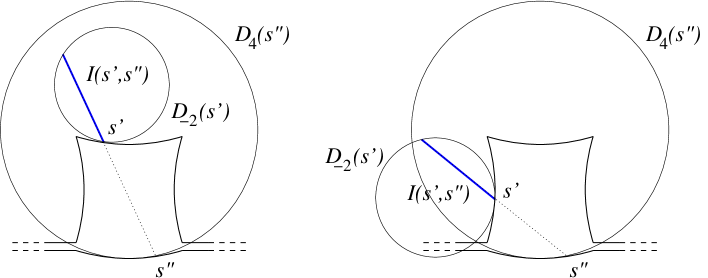
For any $x=(s,\alpha)\in\mathcal{M}$ and $n\in\mathbb{Z}$, denote $x_{n}:=(s_{n},\alpha_{n}):=\mathcal{F}^{n}x$ and let $\tau_{n}$ be the length of the portion of the trajectory (equivalently, the time) between the collisions at $s_{n}$ and $s_{n+1}$ (notice that there can be an arbitrary number of collisions against $\Gamma_{s}$ between $s_{n}$ and $s_{n+1}$). Also, let $k_{n}:=k(s_{n})$ indicate the curvature of $\Gamma$ in $s_{n}$. Analogously, given $v\in T_{x}\mathcal{M}$, denote $v_{n}:=(D\mathcal{F}^{n})_{x}v$. The infinitesimal beam of trajectories determined by $v_{n}$ (and thus by $v$) around $(s_{n},\alpha_{n})$ will have pre- and postcollisional foci denoted, respectively, $F_{n}^{-}:=F^{-}(v_{n})$ and $F_{n}^{+}:=F^{+}(v_{n})$. The corresponding signed distances along the pre- and postcollisional lines are indicated with $f_{n}^{-}$ and $f_{n}^{+}$. The following facts are obvious:

$$F_{n}^{-}=F_{n-1}^{+},$$ (4.3)

$$f_{n}^{-}=-(\tau_{n-1}-f_{n-1}^{+}).$$ (4.4)

For the sake of the notation, let us drop all subscripts 0 and write $k:=k_{0}$, $F^{+}:=F_{0}^{+}$, and so on.

For any $x\in\mathcal{M}$, we introduce the following three cones in $T_{x}\mathcal{M}$:

• $C_{0}(x)$ is the set of all tangent vectors whose correspondent family of rays focuses in linear approximation inside $D_{-2}(s)$. Using the focal distance $f^{+}$,

  $$C_{0}(x):=\left\{v\in T_{x}\mathcal{M}\>\left|\>-\frac{\cos\alpha}{|k|}\leq f^{+}(v)\leq 0\right.\!\right\}.$$ (4.5)

• $C_{1}(x)$ is the set of all tangent vectors whose correspondent family of rays focuses in linear approximation inside $D_{0-}(s)$, i.e., all the divergent families of rays. In projective terms,

  $$C_{1}(x):=\left\{v\in T_{x}\mathcal{M}\>\left|\>-\infty<f^{+}(v)\leq 0\right.\!\right\}.$$ (4.6)

• $C_{2}(x)$ is the set of all tangent vectors whose correspondent family of rays focuses in linear approximation inside $D_{2}(s)\setminus D_{4}^{\circ}(s)$, i.e.,

  $$C_{2}(x):=\left\{v\in T_{x}\mathcal{M}\>\left|\>\frac{\cos\alpha}{2|k|}\leq f^{+}(v)\leq\frac{\cos\alpha}{|k|}\right.\!\right\}.$$ (4.7)

We use the above cones to define piecewise an invariant cone bundle $C:=\{C(x)\}_{x}$. For each $x=(s,\alpha)$, the choice $C(x):=C_{i}(x)$ will depend on $s$, $s_{-1}$, and what happens to the trajectory between the collisions at $s_{-1}$ and $s$.

• If $s\in\Gamma_{d}$, set $C(x):=C_{0}(x)$.

• If $s\in\Gamma_{f}$, there are two subcases:

  • If $s_{-1}\in\Gamma_{f}$, set $C(x):=C_{2}(x)$.

  • If $s_{-1}\in\Gamma_{d}$, there are two further subcases, depending on whether the piece of trajectory between $s_{-1}$ and $s$ has collisions with $\Gamma_{s}$:

    • No collisions with $\Gamma_{s}$ between $s_{-1}$ and $s$: Set $C(x):=C_{1}(x)$.

    • At least one collision with $\Gamma_{s}$ between $s_{-1}$ and $s$: Set $C(x):=C_{2}(x)$.

Clearly $C(x)$ is a measurable function of $x$.

Theorem 4.2

The cone bundle $C$ just defined is eventually strictly invariant relative to the map $\mathcal{F}$.

Proof. We check that $v\in C(x)$ implies $v_{1}\in C(x_{1})$ for all the possible cases $C(x)=C_{i}(x)$, $C(x_{1})=C_{j}(x_{1})$ $(i,j\in\{0,1,2\})$.

• $s,s_{1}\in\Gamma_{d}$. In this case $C(x)=C_{0}(x)$, $C(x_{1})=C_{0}(x_{1})$. $v\in C_{0}(x)$ implies $F^{+}\in D_{-2}(s)$, hence $F_{1}^{-}=F^{+}\in D_{0+}^{\circ}(s_{1})$. By Proposition 3.5, $F_{1}^{+}\in D_{-4}^{\circ}(s_{1})\subset D_{-2}^{\circ}(s_{1})$. This is equivalent to $v_{1}\in C_{0}^{\circ}(x_{1})$—where $C^{\circ}(x)$ represents the interior of $C(x)$ in $T_{x}\mathcal{M}$. We have thus proved strict invariance for this type of collision.

• $s\in\Gamma_{d}$, $s_{1}\in\Gamma_{f}$. Here $C(x)=C_{0}(x)$ but the cone $C(x_{1})$ may take two different forms. We separately check both cases.

  • There are no collisions with $\Gamma_{s}$ between $s$ and $s_{1}$. Then $C(x_{1})=C_{1}(x_{1})$. For $v\in C_{0}(x)$ we have, by condition (4.1), $F_{1}^{-}=F^{+}\in D_{4}(s_{1})$. Proposition 3.5 implies that $F_{1}^{+}\in D_{0-}(s_{1})$, that is, $v_{1}\in C_{1}(x_{1})$. In this case the invariance is not necessarily strict.

  • There are collisions with $\Gamma_{s}$ between $s$ and $s_{1}$, that is, the material point enters a strip before colliding at $s_{1}$. In this case $C(x_{1})=C_{2}(x_{1})$. Since the material point has to travel all the way to the end of the strip and bounce back, $\tau>2l>2/k_{f}$, having used condition (4.2). For $v\in C_{0}(x)$, $f^{+}\leq 0$, hence $f_{1}^{-}=-\tau+f^{+}<-1/k_{f}$. Equivalently, $F_{1}^{-}\in D_{0+}(s_{1})\setminus D_{2}(s_{1})$. By Proposition 3.5, $F_{1}^{+}\in D_{2}^{\circ}(s_{1})\setminus D_{4}(s_{1})$, i.e., $v_{1}\in C_{2}^{\circ}(x_{1})$.

• $s\in\Gamma_{f}$, $s_{1}\in\Gamma_{d}$. Here $C(x_{1})=C_{0}(x_{1})$ and we have two subcases on $C(x)$.

  • $C(x)=C_{1}(x)$. In this case $v\in C(x)$ is equivalent to $f^{+}\leq 0$. Hence $f_{1}^{-}<0$ and $F_{1}^{-}\in D_{0+}^{\circ}(s_{1})$. Therefore (Proposition 3.5) $F_{1}^{+}\in D_{-4}^{\circ}(s_{1})\subset D_{-2}^{\circ}(s_{1})$. Namely $v_{1}\in C_{0}^{\circ}(x_{1})$.

  • $C(x)=C_{2}(x)$. So $v\in C(x)$ means that $F^{+}=F_{1}^{-}\in D_{2}(s)\setminus D_{4}^{\circ}(s)$. We consider two possible types of trajectories:

    • There are no collisions with $\Gamma_{s}$ between $s$ and $s_{1}$. By (4.1), $F_{1}^{-}\in D_{0-}^{\circ}(s_{1})\setminus D_{-2}^{\circ}(s_{1})$. Hence $F_{1}^{+}\in D_{-2}(s_{1})$.

    • There are collisions with $\Gamma_{s}$ between $s$ and $s_{1}$. As in case (II.2), $\tau>2/k_{f}$ and $f^{+}\leq(\cos\alpha)/k_{f}<0$. Thus, $f_{1}^{-}<0$, that is, $F_{1}^{-}\in D_{0+}^{\circ}(s_{1})$. Finally, $F_{1}^{+}\in D_{-4}^{\circ}(s_{1})\subset D_{-2}^{\circ}(s_{1})$.

• $s,s_{1}\in\Gamma_{f}$. Definition (B.1) ensures that $C(x_{1})=C_{2}(x_{1})$. Let us branch out in two subcases depending on $C(x)$.

  • $C(x)=C_{1}(x)$. As in case (III.1), $v\in C(x)$ implies that $f^{+}\leq 0$. Since, by construction of our cross section, there can be no collisions with $\Gamma_{d}$ in the piece of trajectory between $s$ and $s_{1}$, there are only two possibilities: either the particle enters and exits a strip, and thus $\tau>2/k_{f}$; or that piece of trajectory is a chord of the arc $\Gamma_{f}$, and thus $\tau=2(\cos\alpha)/k_{f}$. In either case, $\tau>(\cos\alpha)/k_{f}$ and $f_{1}^{-}<-(\cos\alpha)/k_{f}$, which means that $F_{1}^{+}\in D_{0+}^{\circ}(s_{1})\setminus D_{2}(s_{1})$. By Proposition 3.5, $F_{1}^{+}\in D_{2}^{\circ}(s_{1})\setminus D_{4}(s_{1})$, that is, $v_{1}\in C_{2}^{\circ}(x_{1})$.

  • $C(x)=C_{2}(x)$. The hypothesis $v\in C(x)$ reads $(\cos\alpha)/2k_{f}\leq f^{+}\leq(\cos\alpha)/k_{f}$. Once again, there are two further subcases:

    • There are no collisions with $\Gamma_{s}$ between $s$ and $s_{1}$. In this case, cf. (IV.1), the trajectory between $s$ and $s_{1}$ is a chord of $\Gamma_{f}$ and $\tau=2(\cos\alpha)/k_{f}$. Therefore $f_{1}^{-}=-\tau+f^{+}\leq-(\cos\alpha)/k_{f}$, which implies $F_{1}^{-}\in D_{0+}(s_{1})\setminus D_{2}^{\circ}(s_{1})$. This yields $F_{1}^{+}\in D_{2}(s_{1})\setminus D_{4}^{\circ}(s_{1})$, namely $v_{1}\in C_{2}(x_{1})$.

    • There are collisions with $\Gamma_{s}$ between $s$ and $s_{1}$. $f^{+}$ and $\tau$ are exactly as in case (III.2.2). Refining the estimate that is written there, $f_{1}^{-}<-1/k_{f}<-(\cos\alpha)/k_{f}$, that is, $F_{1}^{-}\in D_{0+}^{\circ}(s_{1})\setminus D_{2}(s_{1})$. This gives $F_{1}^{+}\in D_{2}^{\circ}(s_{1})\setminus D_{4}(s_{1})$.

In order to show that $C$ is eventually strict invariant almost everywhere, we notice that there are only three cases above in which the cone invariance is not strict, namely (II.1), (III.2.1), and (IV.2.1).

In both (II.1) and (III.2.1), nonstrictness can only occur when the external endpoint of $I(s^{\prime},s^{\prime\prime})$ lies on $D_{4}(s^{\prime\prime})$ and $s=s^{\prime}$, $s_{1}=s^{\prime\prime}$, or viceversa—cf. (4.1) and Fig. 6. It is not hard to realize that this situation can only occur for finitely many pairs $(s^{\prime},s^{\prime\prime})$ (at least when the table is optimized, see (5.1) and Fig. 7, there are only two such pairs).

As concerns (IV.2.1), we realize that there can only be a finite number of consecutive collisions of that type, because each such piece of trajectory is a chord of $\Gamma_{f}$ of constant length ($\tau=\tau_{1}$), but $\Gamma_{f}$ is smaller than a semicircle. Q.E.D.

5 Confining the table to a bounded region

In the previous section the table $\Omega$ was constructed starting with two values for $h$ and $k_{d}$, which determined an upper bound on the choice of $k_{f}$, via (4.1), which in turn determined a lower bound on the choice of $l$, via (4.2). The latter condition, in particular, forced the area of $\Omega$ to diverge, as smaller and smaller values are chosen for $k_{f}$.

Now we want to optimize, that is, minimize, the area of the table and to do so we change the order in which its geometric parameters are chosen. Given $k_{d}<0$ and $k_{f}$ sufficiently small, we define the optimal height and the optimal length of the strips, respectively, as:

$$h_{o}:=h_{o}(k_{d},k_{f}):=\min\left\{h\>\left|\>\forall s^{\prime}\in\Gamma_{d},\forall s^{\prime\prime}\in\Gamma_{f},\ I(s^{\prime},s^{\prime\prime})\subset D_{4}(s^{\prime\prime})\right.\!\right\};$$ (5.1)

$$l_{o}:=l_{o}(k_{f})=k_{f}^{-1}.$$ (5.2)

These definitions are well posed, in the sense that a table can be constructed with $h=h_{o}$ and $l=l_{o}$. We call it the optimal table and we think of it as a function of $k_{f}$ ($k_{d}$ is considered fixed once and for all). The optimal table is hyperbolic by Theorem 4.2. The next proposition shows that, as $k_{f}\to 0$, the area of the optimal table is bounded above. (In what follows, the notation $a\sim b$ means that $a=a(k_{f})$, $b=b(k_{f})$ and, as $k_{f}\to 0$, $|a/b|$ is bounded away from $0$ and $\infty$.)

Proposition 5.1

As $k_{f}\to 0$, $h_{o}(k_{f})\sim k_{f}$.

Proof. Since $k_{f}\to 0$ and $k_{d}$ is fixed, we may assume that, given any $s^{\prime\prime}\in\Gamma_{f}$, $D_{4}(s^{\prime\prime})$ easily contains $D_{-2}(s^{\prime})$, for all $s^{\prime}$ in the upper component of $\Gamma_{d}$ (left picture in Fig. 6).

For $s^{\prime}$ belonging to the lateral components of $\Gamma_{d}$, it is not hard to realize that the worst-case scenario is the one depicted in Fig. 7 (or the specular situation w.r.t. the axis of symmetry of $\Omega$): First of all, if $s^{\prime\prime}$ moves to the left and/or $s^{\prime}$ moves upward, $I(s^{\prime},s^{\prime\prime})$ will move towards the interior of $D_{4}(s^{\prime\prime})$, so that (4.1) is always verified. Secondly, setting $h_{o}$ to be the $h$ displayed there, one clearly sees that for $h\geq h_{o}$ (4.1) is verified, while for $h<h_{o}$ it is not.

Figure 7: Finding $h_{o}$, cf. Proposition 5.1.

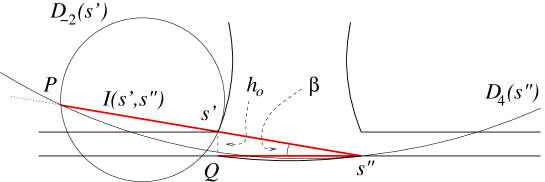
Referring to the notation of Fig. 7, we see that $h_{o}=\tan\beta$ where $\beta$ is the angle between the two chords $s^{\prime\prime}P$ and $s^{\prime\prime}Q$ of $\partial D_{4}(s^{\prime\prime})$. Recalling that, in a circle of radius $r$, the relation between the length $\ell$ of a chord and the angle $\theta$ it makes with the tangent to the circle at each of its endpoints is $\ell=2r\sin\theta$, we have

$$\beta=\arcsin\left(\frac{k_{f}\,c}{2}\right)-\arcsin\left(\frac{k_{f}}{2}\right)\sim k_{f},\quad\mbox{as }k_{f}\to 0.$$ (5.3)

In the above $c$ is the length of $s^{\prime\prime}P$, for which it holds $1<c<2+2k_{d}^{-1}$. This ends the proof since $h_{o}\sim\beta$. Q.E.D.

From a technical point of view, Proposition 5.1 is a consequence of the fact that $\Gamma_{f}$ fails to act as a perturbation of a semidispersing component only for a few trajectories, whose corresponding beams need to be defocused by visiting the long strips. As $k_{f}\to 0$, this phenomenon concerns fewer and fewer trajectories, but its fix requires more and more space. Proposition 5.1 tells us that the trade-off between the two effects balances out.

If a hyperbolic billiard table with a flatter and flatter focusing component need not become bigger and bigger in terms of area, one might hope that it need not in terms of diameter, either. In our particular table, one would like to redesign the strips so that their area is better placed in the plane and can be included in a fixed compact region. In the remainder of the section we show that this is possible, for example by bending the strips around the bulk of the billiard (see Fig. 2).

Figure 8: Construction of a spiral as a union of trapezoids.

Let us describe this construction with the help of Fig. 8. Substitute each strip of $\Omega$ with a polygonal modification given by the union of $N$ adjacent right trapezoids $T_{1},T_{2},\ldots,T_{N}$, where $N$ will be specified later depending on $k_{f}$. $T_{1}$ is placed so that its shorter leg coincides with the opening towards the bulk of $\Omega$: its height is then $h_{1}:=h\geq h_{o}$. The length of the shorter base is denoted $l_{1}$ and the two nonright angles are denoted $\pi/2+\gamma_{1}$ and $\pi/2-\gamma_{1}$, with $0<\gamma_{1}<\pi/2$. This causes the longer leg to measure $h_{2}:=h_{1}/\cos\gamma_{1}$. The longer leg of $T_{1}$ is then used as the shorter leg of the next trapezoid, $T_{2}$, in the way depicted in Fig. 8. The construction continues recursively, as values for $l_{i}$, $\gamma_{i}$ (and therefore $h_{i+1}:=h_{i}/\cos\gamma_{i}$) are generated with each new trapezoid $T_{i}$. We call the resulting region a polygonal spiral, or simply spiral.

There are two of them, and they need not be equal, so we denote $N^{R},h_{i}^{R},l_{i}^{R},\gamma_{i}^{R}$, and $N^{L},h_{i}^{L},l_{i}^{L},\gamma_{i}^{L}$, the parameters of the right and the left spiral, respectively. These will be determined later depending on $h_{o}$ and $l_{o}$, thus ultimately on $k_{f}$. We will see to it that the following conditions hold:

• The spirals turn counterclockwise at each corner.

• They have no self-intersections, or intersections between them or with the bulk of $\Omega$.

• For $\epsilon\in\{R,L\}$, all angles $\gamma_{i}^{\epsilon}$ are rational multples of $\pi$.

• There exists an absolute constant $K_{1}$ (i.e., $K_{1}$ does not depend on anything, including $k_{f}$) such that, for $\epsilon\in\{R,L\}$,

  $$h_{N^{\epsilon}}^{\epsilon}\leq K_{1}h_{o}.$$ (5.4)

• There exists an absolute constant $K_{2}>1$ such that

  $$l_{o}\leq\sum_{i=1}^{N^{\epsilon}}l_{i}^{\epsilon}\leq K_{2}\,l_{o}.$$ (5.5)

• There exists an absolute constant $K_{3}$ such that, $\forall i=1,2,\ldots,N^{\epsilon}$,

  $$\frac{\tan\gamma_{i}^{\epsilon}}{l_{i}^{\epsilon}}\leq\frac{K_{3}}{h_{i}^{\epsilon}}.$$ (5.6)

  (The l.h.s. above is a measure of the “curvature” of the spiral at the $i$-th corner.)

Under the above conditions the area of each spiral is bounded, as $k_{f}\to 0$, because, dropping the superscript $\epsilon$,

$$\frac{1}{2}\sum_{i=1}^{N}(2l_{i}+h_{i}\tan\gamma_{i})h_{i} \leq \frac{2+K_{3}}{2}\sum_{i=1}^{N}l_{i}h_{i}$$

$$\leq \mbox{const }l_{o}h_{N}$$

$$\leq \mbox{const }l_{o}h_{o}\sim 1;$$

having used, in this order, (5.6), (5.5), and (5.4). Also, defining $(\mathcal{M},\mathcal{F},\mu)$ as in Section 4, namely, as the dynamical system corresponding to the cross section $\mathcal{M}$ of all line elements based in $\bar{\Gamma}=\Gamma_{f}\cup\Gamma_{d}$, we have:

Proposition 5.2

$\mathcal{M}$ is a global cross section for the billiard flow and $(\mathcal{M},\mathcal{F},\mu)$ is hyperbolic.

Proof. First of all, $\mathcal{F}$, as the first-return map onto $\mathcal{M}$, is well-defined almost everywhere (e.g., by the Poincaré Recurrence Theorem).

To prove that $\mathcal{M}$ is a global cross section, we need to show that a.a. billiard trajectories have collisions against $\bar{\Gamma}=\Gamma_{f}\cup\Gamma_{d}$. This is easy if we use a well-known result from the theory of polygonal billiards [ZK, BKM]: Let $P$ be the union of the two spirals plus $R$, which is the rectangle (of base 1 and height $h$) joining the open ends of the spirals. $P$ is a rational polygon, meaning that all its angles are rational multiples of $\pi$. In a rational polygonal billiard, all but countably many values of the velocity $u\in S^{1}$ are minimal, in the sense that any nonsingular flow-trajectory in configuration space (i.e., the set $\{q(t)\}_{t\in\mathbb{R}}$, provided that it contains no corner of $P$), with initial velocity $u$, is dense in $P$ [ZK, BKM]. This implies that for a.a. initial conditions $(q,u)$, with $q\in P$, the billiard trajectory in $P$ hits the boundary of $R$, which means that the true billiard trajectory, relative to the table $\Omega$, hits $\bar{\Gamma}$.

As for the second assertion of Proposition 5.2, we need the following lemma, which will be proved later.

Lemma 5.3

A material point that enters a spiral will travel all the way to the end of the spiral. In particular, if $\tau$ is the travel time between the last collision before entering the spiral and the first collision after exiting it (a.a. trajectories eventually exit the spiral), then $\tau>2l_{o}=2/k_{f}$.

Lemma 5.3 shows that Theorem 4.2 (and thus Theorem 3.1) applies to the present case as well, since its proof only requires of trajectories visiting a strip—or a spiral—that the travel time $\tau$ be larger than $2/k_{f}$. (Note that, since the spirals are two polygons, they will have no effect on the hyperbolic features of an infinitesimal beam of trajectories, just like the two strips. The only, inconsequential, difference is that the spirals have more corners than the strips, resulting in more discontinuity lines in $\mathcal{M}$.) Q.E.D.

Proof of Lemma 5.3. The first assertion is an easy consequence of our design, since a point that enters $T_{i}$ through the shorter leg will necessarily exit it through the longer leg, thus entering $T_{i+1}$ through the shorter leg, and so on. As for the second assertion, clearly $\tau$ will be larger than twice the sum of the lengths of the shorter bases of the trapezoids. By (5.5), this sum is bounded below by $l_{o}$. Q.E.D.

Figure 9: The double spiral (right picture) “wrapping” around the bulk of $\Omega$ (left picture). The double spiral starts when the two spirals coming out of the bulk of $\Omega$ join. Its initial ray is $r_{0}$, its initial (total) width is $w_{0}$, each turn amounts to an angle $\bar{\gamma}=2\pi/\bar{N}$, and the number of rounds is $M$. The point $A$ is the center of the double spiral.

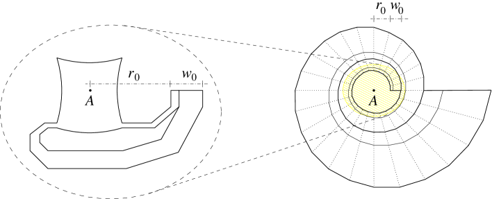
Let us finally give the exact construction of the two spirals. First of all, we design the spirals to become adjacent after a finite number of turns, say $m^{R}$ turns for the right spiral and $m^{L}$ turns for the left spiral (left picture of Fig. 9); $m^{R}$ and $m^{L}$ are absolute constants. We say that the two spirals have now joined in a regular double spiral, since they will keep adjacent as they spiral outwards in the regular way shown in the right picture of Fig. 9. More precisely, all trapezoids $T_{i}^{R}$, with $i\geq m^{R}$, and $T_{i}^{L}$, with $i\geq m^{L}$, are similar, and are defined by $\gamma_{i}^{\epsilon}=\bar{\gamma}:=2\pi/\bar{N}$, where $\bar{N}$ is an integer (depending on $h_{o}$) to be determined momentarily. The double spiral is also defined so that its initial ray (meaning the distance from the border of the spiral to its center $A$, see Fig. 9) is $r_{0}$, an absolute constant so large that intersection with the bulk of $\Omega$ is avoided.

At each next corner, the ray (that is, the distance between that corner and $A$) increases by a factor $1/\cos\bar{\gamma}$. Therefore, after the first round, the ray has become $r_{\bar{N}}:=r_{0}(\cos\bar{\gamma})^{-\bar{N}}$. Since the spiral wraps around itself tightly (i.e., leaving no area uncovered), its initial width is

$$w_{0}:=r_{0}\left(\left(\cos\frac{2\pi}{\bar{N}}\right)^{-\bar{N}}\!\!\!-1\right).$$ (5.8)

On the other hand, in the place where the left and right spirals join to start the double spiral, one sees that

$$w_{0} = h_{m^{R}}^{R}+h_{m^{L}}^{L}$$

$$= \left(\prod_{i=1}^{m^{R}}\frac{1}{\cos\gamma_{i}^{R}}+\prod_{i=1}^{m^{L}}\frac{1}{\cos\gamma_{i}^{L}}\right)h$$

$$=: K_{4}\,h.$$

$K_{4}$ is an absolute constant if we prescribe that, for $i=1,\ldots,m^{\epsilon}$, the angles $\gamma_{i}^{\epsilon}$ are rational multiples of $\pi$ and stay fixed while $k_{f}\to 0$ (this is geometrically possible, cf. Fig. 9, left picture). The last two equations imply that

$$h=h_{1}=\frac{r_{0}}{K_{4}}\left(\left(\cos\frac{2\pi}{\bar{N}}\right)^{-\bar{N}}\!\!\!-1\right).$$ (5.10)

Given $k_{f}$ sufficiently small, we use (5.10) to define both $h$ and $\bar{N}$, keeping in mind that we want $h_{o}\leq h\leq K_{1}h_{o}$, cf. (5.4). We need this estimate from elementary calculus:

$$\lim_{n\to+\infty}\,\frac{n}{2\pi^{2}}\left(\left(\cos\frac{2\pi}{n}\right)^{-n}\!\!\!-1\right)=1.$$ (5.11)

So the r.h.s. of (5.10) decreases like $1/\bar{N}$, as $\bar{N}\to\infty$. This ensures that, given any sufficiently small $h_{o}$, there exists an $\bar{N}=\bar{N}(h_{o})$ such that the corresponding $h=h(h_{o})$, as in (5.10), verifies $h_{o}\leq h\leq 2h_{o}$. Since $h_{o}=h_{o}(k_{f})$, we rename these two values, respectively, $\bar{N}(k_{f})$ and $h(k_{f})$ (abbreviated in $\bar{N}$ and $h$ when there is no risk of confusion). Clearly, as $k_{f}\to 0$,

$$h(k_{f})\sim h_{o}\sim k_{f};$$ (5.13)

$$\bar{N}(k_{f})\sim h^{-1}\sim k_{f}^{-1}.$$

Together with $r_{0}$, $h_{m^{R}}^{R}$ (equivalently $h_{m^{L}}^{L}$) and $\bar{\gamma}$ (equivalently $\bar{N}$), the fourth and last parameter that completely determines the double spiral is $M$, which is defined as the number of complete rounds the spiral makes. (Once $M$ is determined, the total number of trapezoids in the right and left spirals is given by

$$N^{\epsilon}=m^{\epsilon}+M\bar{N},$$ (5.14)

for $\epsilon=R$ and $\epsilon=L$, respectively.) Choosing

$$M=M(k_{f}):=\left[\frac{l_{o}}{2\pi r_{0}}\right]+1=\left[\frac{1}{2\pi r_{0}k_{f}}\right]+1$$ (5.15)

(where $[\,\cdot\,]$ is the integer part of a positive number) ensures that the first inequality of (5.5) is verified, since $\sum_{i}l_{i}^{\epsilon}>M2\pi r_{0}>l_{0}$. Also, for $\epsilon\in\{R,L\}$,

$$h_{N^{\epsilon}}=h_{m^{\epsilon}}^{\epsilon}(\cos\bar{\gamma})^{-M\bar{N}}\sim h_{m^{\epsilon}}^{\epsilon}\sim h_{o},$$ (5.16)

as $k_{f}\to 0$, because of (5.11) and the fact that $M\sim k_{f}^{-1}$ (whence $M\bar{N}\sim\bar{N}^{2}$). The above verifies (5.4). As for the second inequality of (5.5), we know that the trapezoids $T_{i}^{\epsilon}$, for $i\geq m^{\epsilon}$, are similar. Therefore, in the limit $k_{f}\to 0$, we obtain

$$\sum_{i=1}^{N^{\epsilon}}l_{i}^{\epsilon} \sim \sum_{i=m^{\epsilon}}^{N^{\epsilon}}l_{i}^{\epsilon}\>=\ l_{m^{\epsilon}}^{\epsilon}\sum_{j=0}^{M\bar{N}-1}(\cos\bar{\gamma})^{-j}$$

$$\sim \tan\bar{\gamma}\,\frac{(\cos\bar{\gamma})^{-M\bar{N}}-1}{(\cos\bar{\gamma})^{-1}-1}$$

$$\sim \bar{N}^{-1}\frac{1}{\bar{N}^{-2}}\sim\bar{N}\sim k_{f}^{-1}$$

$$\sim l_{o},$$

which proves (5.5). In the above we have used (5.13) and the evident geometric equalities $l_{m^{R}}^{R}=r_{0}\tan\bar{\gamma}$ and $l_{m^{L}}^{L}=(r_{0}+h_{m^{R}}^{R})\tan\bar{\gamma}$ (Fig. 9). Finally, (5.6) holds because, for all $i\geq m^{\epsilon}$, $l_{i}^{\epsilon}/h_{i}^{\epsilon}$ is constant, while $\gamma_{i}^{\epsilon}=\bar{\gamma}\to 0$, as $k_{f}\to 0$.

The next and last result, whose proof is apparent, emphasizes the motivation behind the constructions of Section 5.

Proposition 5.4

The table $\Omega=\Omega(k_{f})$ defined before is contained in a bounded region of the plane independent of $k_{f}$.

References

- [BKM] C. Boldrighini, M. Keane and F. Marchetti, Billiards in polygons, Ann. Probab. 6 (1978), no. 4, 532–540.
- [B1] L. A. Bunimovich, On billiards close to dispersing, Math. USSR Sb. 23 (1974), 45–67.
- [B2] L. A. Bunimovich, On the ergodic properties of nowhere dispersing billiards, Comm. Math. Phys. 65 (1979), no. 3, 295–312.
- [B3] L. A. Bunimovich, On absolutely focusing mirrors, in: Ergodic Theory and related topics, III (Gustrow, 1990), edited by U. Krengel et al., Lecture Notes in Math. 1524, Springer, Berlin (1992), 62–82.
- [BL] L. Bussolari and M. Lenci, Hyperbolic billiards with nearly flat focusing boundaries. II, in preparation.
- [CM] N. Chernov and R. Markarian, Chaotic billiards, Mathematical Surveys and Monographs, 127. American Mathematical Society, Providence, RI, 2006.
- [De] G. Del Magno, Ergodicity of a class of truncated elliptical billiards, Nonlinearity 14 (2001), no. 6, 1761–1786.
- [D] V. J. Donnay, Using integrability to produce chaos: billiards with positive entropy, Comm. Math. Phys. 141 (1991), no. 2, 225–257.
- [K] A. Katok (with the collaboration of K. Burns), Infinitesimal Lyapunov functions, invariant cone families and stochastic properties of smooth dynamical systems, Ergodic Theory Dynam. Systems 14 (1994), no. 4, 757–785.
- [KS] A. Katok and J.-M. Strelcyn (in collaboration with F. Ledrappier and F. Przytycki), Invariant manifolds, entropy and billiards; smooth maps with singularities, Lecture Notes in Math. 1222, Springer-Verlag, Berlin-New York, 1986.
- [LW] C. Liverani and M. Wojtkowski, Ergodicity in Hamiltonian systems, in: Dynamics Reported: Expositions in Dynamical Systems (N.S.), 4, Springer-Verlag, Berlin, 1995.
- [M1] R. Markarian, Billiards with Pesin region of measure one, Comm. Math. Phys. 118 (1988), no. 1, 87–97.
- [M2] R. Markarian, Non-uniformly hyperbolic billiards, Ann. Fac. Sci. Toulouse Math. (6) 3 (1994), no. 2, 223–257.
- [RT] V. Rom Kedar and D. Turaev, Big islands in dispersing billiard-like potentials, Phys. D 130 (1999), no. 3-4, 187–210.
- [S] Ya. G. Sinai, Dynamical systems with elastic reflections, Russ. Math. Surveys 25 (1970), no. 2, 137–189.
- [TR] D. Turaev and V. Rom Kedar, Soft billiards with corners, J. Statist. Phys. 112 (2003), no. 3-4, 765–813.
- [W1] M. Wojtkowski, Invariant families of cones and Lyapunov exponents, Ergodic Theory Dynam. Systems 5 (1985), no. 1, 145–161.
- [W2] M. Wojtkowski, Principles for the design of billiards with nonvanishing Lyaponov exponents, Comm. Math. Phys. 105 (1986), no. 3, 391–414.
- [ZK] A. N. Zemlyakov and A. B. Katok, Topological transitivity of billiards in polygons, Math Notes 18 (1975), no. 1–2, 760–764 (1976).