Preface

The main reason to study B meson decays is their sensitivity to the flavor structure of nature. Indeed, the fact that the $b$ quark is so heavy makes B physics a rich source of very different processes, and leads to a very rich phenomenology. An additional consequence of the large mass of the $b$ quark, that makes B decays interesting on the theoretical side is the fact that the always troublesome strong interaction effects can be handled within a heavy-quark expansion, allowing for theoretical predictions of acceptable accuracy. In fact, one of the differences between B- and D-physics is that decays of D mesons are theoretically much “dirtier”. B decays have therefore triggered intensive research on the QCD side, that has witnessed a huge progress in the last decade.

One of the main points in the B physics program is the search for physics beyond the Standard Model (SM). To that end, a number of dedicated facilities have been taking data for many years, achieving a long list of new discoveries. Specifically, the B-factories Babar and Belle, and the hadronic machine at Tevatron, with its experiments CDF and D0, have made this possible. Joint work by theorists and experimentalists has led to the appearance of several puzzles in B decays which could be interpreted to be due to New Physics (NP). However, these may as well disappear as more accurate measurements are made, or new understanding is accomplished on the theoretical side. The imminent start up of the Large Hadron Collider (LHC), with its B physics experiment LHCb, and the possibility of a super-B factory will certainly play a very exciting role in the search for physics beyond the SM, and once NP is found, in understanding its nature.

The motivations that guide us in the search for NP –that so many times have triggered false alarms– are many. They can be classified in three major classes. Motivations belonging to the first class are related to observational facts that our theory (the SM) cannot reproduce. The baryon asymmetry in the universe, as understood by now, requires the three so-called Sakharov conditions. One of such conditions is an amount of CP violation that the SM cannot account for. The solution most probably requires new sources of CP violation. The presence of dark matter and dark energy is also an observational fact that has not found its solution within the standard theory, and which points towards the existence of new particle content.

Motivations belonging to the second class are related to observations that can in principle fit into the theory but which would then seem extremely unnatural. The SM predicts two independent sources of CP violation in strong interactions. One is driven by the presence of instantons and the other comes from the diagonalization of the quark mass matrix. The measurement of the electric dipole moment of the neutron tells us that these two –in principle unrelated– contributions must cancel to one part in $10^{9}$. The classical solution to this strong CP-problem is to postulate a $U(1)_{A}$ (Peccei-Quinn) symmetry that dynamically sets this small number to zero. This solution requires the existence of (at least) a new particle, the axion. The hypothesis of inflation, introduced originally as a solution to the horizon and flatness problems, is pretty much accepted by the physics community nowadays. However, whatever drives inflation is still unknown, and again the many proposed mechanisms involve physics beyond the SM. The most striking fine-tuning problem is maybe the one related to the cosmological constant, which states that several unrelated contributions to the vacuum energy and the bare cosmological constant must cancel to one part in $10^{120}$ in order to agree with observations, which is preposterous. The Higgs fine-tunning problem arises from the instability of the mass of a scalar particle to radiative corrections. The difference between the electroweak (EW) and the planck scales requires a fine-tunning of one part in $10^{30}$. Supersymmetry solves this problem protecting the mass of the scalars, which are not protected by gauge invariance, but the solution might as well be ultimately of different nature. In any case it should manifest itself as NP at $\sim 1{\rm TeV}$.

Motivations belonging to the third class are not related to problems, but to unanswered issues. The inclusion of gravity in the standard picture is an issue that has led to the study of extra dimensions and string theory. A thorough theoretical investigation over decades indicates that quantum gravity can only be merged with the SM together with a significant amount of NP. The SM suffers by itself from its own unanswered issues, more related to this thesis than the problem of gravity. The SM contains 28 free independent parameters, a feature that goes directly against the quest for unification that motivated its foundations. An attempt to reduce the number of gauge parameters, through the gauge coupling unification, requires Supersymmetry and a long list of new particles, introducing even more parameters. From the 28 free parameters in the SM, 22 are directly related to the flavor sector. The hierarchy of the CKM matrix and the hierarchy in the masses of the quarks and leptons of different families should have an explanation beyond the SM, and constitutes part of the SM flavor problem. The existence of 3 generations of quarks and leptons is intriguing, and the existence of a fourth family is neither theoretically nor experimentally excluded. The fact that neutrinos are not massless provides new puzzles concerning the mixings, hierarchies and flavor violations in the leptonic sector to which any NP would have a definite impact.

So it is clear that the search for new physics is strongly motivated. Past experience has also taught us that purely theoretical arguments are a powerful tool that leads to actual discovery. The positron was predicted by Dirac as a product of the unification of relativity and quantum mechanics. The charm quark was postulated in order to provide a GIM mechanism to suppress FCNC’s. The third family of quarks was postulated in order to allow CP violation through the KM mechanism. The weak gauge bosons W, Z were predicted with the right masses as a realization of the GWS theory of weak interactions. These and other successes are the proof that the theoretical method is in the right track, and that research on the problems mentioned above will bring discoveries as impressive as old problems did in the past. However, as important as theoretical elucidation might be, experiment is the only way we get to know the world. Both must be connected through the ever crucial link: phenomenology.

The role of flavor physics is central to this enterprise at the phenomenological level. The search for new physics begins with the understanding of the SM itself, and the precise determination of its parameters. The majority of these parameters are flavor parameters that are not very well determined in the present, but where impressive progress has been made (see Fig.1). In fact the determination of the flavor parameters of the SM will soon become of the precision type. Flavor parameters can only be determined through flavor physics, and the determination of the flavor parameters is necessary in order to infer not only quantitative but also qualitative aspects of the physics above the EW scale, and of the mechanism responsible for the flavor structure that we see at low energies.

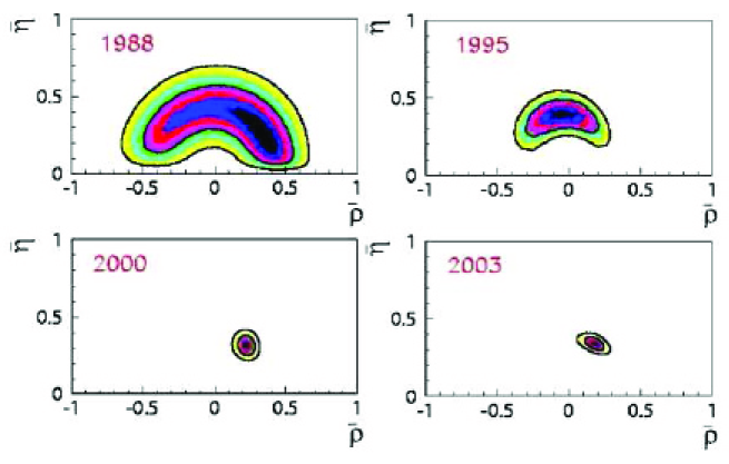
Figure 1: The progress in the determination of the Unitarity Triangle.

The importance of flavor physics cannot be overestimated. If there is really new physics at the TeV scale, it will be most probably detected at the imminent LHC at CERN within 2 to 5 years from now. However, revealing the true nature of those new particles is a much more uncertain task. The relevance of the discovery of NP is certainly to find the answers to the problems raised above. Will the discovered new particles provide a clue about the origin of flavor? Or about the mechanism of electroweak symmetry breaking (EWSB)? Or a sensible reason for the existence of large hierarchies? As far as we know all these problems may be related, or they may be as well completely disconnected. Will it be clear from the beginning that we are discovering Supersymmetry, or extra dimensions, or something else? Indeed, the direct search for new particles is an important but not the only part of the New Physics program. And this is where flavor physics comes at hand. Flavor physics constitutes a powerful arena on which to investigate detailed aspects and properties of the new physics and its possible role on the observed phenomenology. Indeed, flavor physics has already provided important constraints on the properties of the new physics concerning its CP and flavor violating structure. It has even raised its own problems. The suppression of flavor-changing neutral currents (FCNC’s) is an observational fact that introduces a strong requirement in the flavor nature of the new physics. Without any mechanism that suppresses FCNC processes, any generic scenarios for NP should be suppressed by a scale larger than $\sim 10^{3}{\rm TeV}$. Therefore, any TeV NP must have a very specific flavor structure in order to satisfy the flavor bounds. This is the NP flavor problem. The non standard CP violating phases that appear, for example, in supersymmetry, are constrained to be of order $10^{-3}$. If supersymmetry is invoked to tame the hierarchy problem of the Higgs mass, it should provide a reasonable explanation for the smallness of these phases. Without a mechanism of this sort, such scenarios of supersymmetry are problematic.

In the Standard Model, the description of CP violation is given by the CKM mechanism. This mechanism is extremely economic, allowing for one single CP violating weak phase. Therefore, within the SM CP is violated “minimally”. This provides us with an incredibly predictive framework, which can be tested meticulously by over-constraining the four parameters of the CKM matrix. It is somehow surprising, and certainly remarkable, that this simple picture is so far in quantitative agreement with all laboratory experiments made up to now. The combination of all observables that constrain the CKM matrix is usually carried out through a fit to the apex of the Unitarity Triangle (UT). Today, this fit defines a consistent and very much constrained Unitarity Triangle (see Fig.2), giving the following results for the real ($\bar{\rho}$) and imaginary ($\bar{\eta}$) parts of its apex:

$$\bar{\rho}=0.164\pm 0.029\ ,\quad\bar{\eta}=0.340\pm 0.017$$ (1)

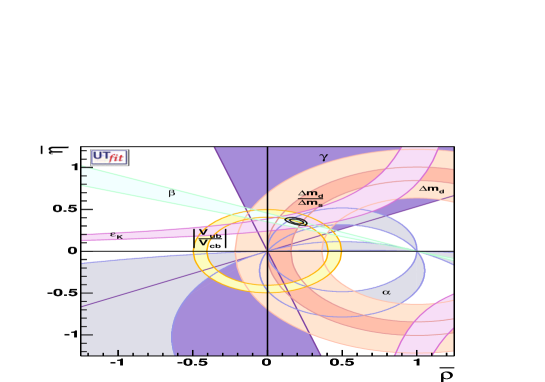
Figure 2: Fit to the apex of the standard Unitarity Triangle as of October 2007.

The general hope, however, is that more precise measurements and more precise theoretical predictions will at some point reveal some inconsistency. Once a number of well identified observables have been observed to deviate from the SM expectations, they can be used to study the nature of the New Physics. If these are flavor observables, their deviations will be a holy grail for the understanding of the flavor structure of the new physics that might be directly observed at the LHC.

There is a major theoretical difficulty, however, that affects the determination of the SM parameters and the search for New Physics. This difficulty is related to the non-perturbative nature of QCD at low energies. Without it, the question of whether the SM is in agreement with all the measured observables would be a strict matter of experimental precision (combined possibly with a perturbative calculation up to a large enough number of loops).

There are several features of strong interactions that are well known. First, at high energies the hadrons show a “partonic” structure, as can be inferred from deep inelastic scattering experiments, revealing the existence of quarks. This picture of hadrons in terms of “partons” unravels one of the characteristic features of strong interactions, which is asymptotic freedom. Second, the mere existence of hadrons means that for some reason the elementary quarks from which they are composed, are confined. This is verified by the fact that quarks are not observed in isolation, and the fact that colored “objects” are not observed either. Although quark confinement and color confinement are slightly different concepts, it is clear that evidence favors both. Both features, asymptotic freedom and confinement, can be understood qualitatively in terms of the scaling of the strong interaction strength. In this picture, strong interactions are very strong at long-distances, and they decrease with increasing energy to become very weak at short distances.

The reasons to believe that QCD is the theory of strong interactions are compelling. First, the theory is formulated exactly as it is understood nowadays that a relativistic quantum theory of particle interactions should be. It is a renormalizable quantum field theory based on a local gauge principle. Its gauge group is SU(3), where the fact that there are 3 colors is known from $e^{+}e^{-}\to\,{\rm hadrons}$. From the non abelian nature of the gauge group it follows that, at least for a reasonable number of fermion families, the theory is asymptotically free, and that the coupling constant increases at long distances. Moreover, perturbative computations in QCD are very successful at large energies, where perturbation theory applies nicely. So, at least in the perturbative regime, QCD shows the qualitative features of strong interactions and reproduces quantitatively the experimental results.

In the non-perturbative regime, however, things are less clear. First, it has not been proven that QCD implies confinement. Second, it is not known how to extract the hadronic spectrum from QCD. For example, the Bethe-Salpeter equation, as a dictionary that translates from quarks to hadrons and back, it is extremely difficult to solve. Despite these formal deficiencies, however, a great progress has been made since the development of QCD in the 70’s, and many qualitative features of strong interactions at low energies can be connected to features of “QCD-like” theories. For example, the large-N limit of QCD is able to give qualitative explanations for the Zweig’s rule, the dominance of the leading fock states in the mesons, or the success of Regge phenomenology. Other successes of QCD itself in the non perturbative regime concern predictions derived for example from QCD sum-rules or from lattice simulations.

Concerning the strong interactions in B decays, the progress has been driven by the observation that one can perform a perturbative expansion in the small parameter $\Lambda_{QCD}/m_{b}$. The first step was the development of an effective theory for mesons containing heavy quarks, called Heavy Quark Effective Theory (HQET). This theory manifests explicitly the symmetries that arise in the heavy quark limit and allows, for example, to relate different heavy-heavy form factors to a single (Isgur-Wise) function. For inclusive B decays, the large value of the $b$ mass allows to use the so called Heavy Quark Expansion (HQE), which predicts, for example, that the inclusive decay of a B meson is dominated by the partonic decay of the b quark alone. In the case of exclusive decays, the establishment of a power counting in terms of $\Lambda_{QCD}/m_{b}$ led to the development of the QCD factorization approach that has been used extensively to make predictions for all two body hadronic, and radiative B decays. Finally, a consistent effective field theory of exclusive and inclusive heavy meson decays at large momentum transfer has been formulated under the name of Soft Collinear Effective Theory (SCET). However, much has to be done before we are able to give theoretical predictions for exclusive hadronic decays with uncertainties at the percent level.

In this thesis I present some topics related to my work in non-leptonic decays of $B$ mesons. It is divided it two major parts. The first part is an overview of the basic matters that constitute the background on which the original work is based. Such a general overview is not an easy task in this field, since there are many topics involved, some of them very well established, and some of them not so much. Therefore I might have been too extensive on very well known areas, maybe short in topics that require more explanation, I may have been repetitive on some parts and on the contrary have skipped completely things that some people will miss. However, I believe that the whole text is quite self-contained, and that this first part constitutes a rather complete link to the second part. I have divided this part in three chapters: first I discuss the weak effective hamiltonian in $B$ physics, both in the context of the SM and for the study of NP. Then I present the concept of factorization for the computation of matrix elements, and also the use of flavor symmetries as an alternative to direct computations. Finally I present the theory of CP violation in meson decays. All these three topics are necessary ingredients in the work presented in the second part.

The second part of this thesis contains a series of applications of the theory presented in the first part. It is based on some papers that have been published within the last three years. These chapters are intimately related, but constitute different “topics” in the field; this is what motivates the title of this thesis. The central issue is the study of $B_{s}\to KK$ modes within and beyond the SM, but it requires an interconnection with the whole grand compact field of flavor physics in general, and in particular of $B$ physics. I hope the concepts are written clearly and the structure of this thesis makes it easy to read, and easy to pose questions, and comments.

Finally, I would like to acknowledge my collaborators, David London, Seungwon Baek, Sebastien Descotes-Genon and Rafel Escribano for nice collaborations and thousands of mails of enlightening content. I am also indebted to the theory groups at Dortmund and Rome for the hospitality during my stays there, where also some part of this work was done. Many thanks also to Felix Schwab, who so kindly made a thorough reading of the first part of this thesis and contributed with intelligent comments and suggestions. I am particularly grateful to Guido Martinelli, Bernardo Adeva, Sebastien Descotes, Santi Peris, Joan Soto, Gudrun Hiller and Ramon Miquel for reading the thesis, and participating as members of the committee. Some of them, specially Guido, contributed with important suggestions, improving further the quality of this writing. Very special thanks go to my thesis advisor, Joaquim Matias, with whom I’ve had endless conversations about physics and life since April 2004, and has gone through painful revisions of this text. I can hardly imagine a better tutor. Personal acknowledgements have been kept personal.

Part I Fundamentals

Chapter 1 Effective Hamiltonians for B physics

B physics describes weak decays of B mesons. This means that it studies physical processes which involve simultaneously –at least– three different energy scales. First, the fact that they are weak decays implies that they involve the scale of weak interactions, given by the mass of the $W$ boson, $M_{W}$. Second, since the energy of the process is that of the decaying meson, a second scale involved is the mass of the B meson $m_{B}$. Third, the fact that we are dealing with mesons implies that the physics of strong interactions of bound states is also important. The scale introduced in this case is the hadronic scale $\Lambda_{QCD}$. Moreover, since we are looking for new physics, it is reasonable to allow for the existence of at least another energy scale, $\Lambda_{NP}$, the scale at which the SM breaks down as an effective theory.

The mere existence of several energy scales does not by itself recall for the use of effective hamiltonians. The utility of an effective theory arises when two different physical phenomena are mostly independent of one another because they operate at completely different scales. For example, the vibration of the atoms in a macroscopic object is too fast to affect at all the movement of the object, and the movement of the object is too slow to affect at all the vibration of its atoms, so both physical processes can be studied independently. Weak decays of B mesons are most suitably studied within an effective theory approach because of the large separation between the energy scales involved:

$$\Lambda_{QCD}\ll m_{B}\ll M_{W},\ \Lambda_{NP}$$ (1.1)

In fact, $\Lambda_{QCD}\sim 0.2-1\,{\rm GeV}$, $m_{B}\sim 5\,{\rm GeV}$, $M_{W}\sim 100\,{\rm GeV}$ and $\Lambda_{NP}>{\rm few\ TeV}$. The large scale of weak interactions and New Physics with respect to the mass of the B meson motivates the use of the weak effective Hamiltonian, which is introduced in this chapter. The low scale of the strong interaction inside hadrons with respect to the mass of the B meson (or the b quark in this case) is what motivates the use of Heavy Quark Effective Theory (HQET). A classical exhaustive reference for HQET is the review by Neubert [2]. Other scales that appear in exclusive decays of B mesons are related to the collinear and hard-collinear degrees of freedom, that introduce a scale of order $m_{b}\Lambda_{QCD}$ which motivates the use of Soft Collinear Effective Theory (SCET). The theoretical and phenomenological importance of this recent development calls at least for a set of references linked to its formulation [3, 4, 5, 6, 7, 8].

1.1 The Weak Effective Hamiltonian

The study of hadronic weak decays is rooted to the concept of the effective weak Hamiltonian. It describes weak interactions at low energy, relevant for energies below $M_{W}$, and it has the structure of an expansion of local effective operators (OPE):

$$\mathcal{H}_{\rm eff}=\frac{G_{F}}{\sqrt{2}}\sum_{i}C_{i}(\mu)\,Q_{i}$$ (1.2)

It can be regarded as a generalization of the Fermi theory to include all quarks and leptons and the electroweak and strong interactions described by the SM. Furthermore, it constitutes a suitable framework for the inclusion of physics beyond the SM. The effective Hamiltonian is defined so that the amplitude is given by

$$A(i\to f)=\langle f|\mathcal{H}_{\rm eff}|i\rangle=\frac{G_{F}}{\sqrt{2}}\sum_{i}C_{i}(\mu)\langle f|Q_{i}(\mu)|i\rangle$$ (1.3)

When dealing with such an effective description, there are two ways to proceed. The first one is to treat the coefficients in the OPE as unknown phenomenological parameters, to be measured or constrained through experiment. Once these are measured, the effective theory can be tested by checking its predictions over different observables. This approach was the one followed in Fermi’s theory, and it is relevant when the fundamental theory is unknown. Yet the SM itself is often seen as an effective theory in this context. Alternatively, if the underlying theory is known (or assumed) then these coefficients can be calculated in terms of the fundamental parameters.

When following the later approach, one must compute the amplitudes in the full theory. One will, in general, encounter the typical divergencies that can be absorbed through conventional renormalization, and that introduces a renormalization scale $\mu$. When dealing with the effective theory, the inclusion of QCD effects also introduces divergencies. Some of them can be reduced through field renormalization; however, the resulting expressions are still divergent. Hence, one is forced to introduce an operator renormalization, to remove these divergencies. This process generically mixes different operators in the OPE, in such a way that new operators can arise that were not present at tree level (without QCD corrections). It is therefore important to work with a basis of operators which is “closed” under renormalization.

There are several very important issues related with the appearance of a renormalization scale in the OPE. First, the full amplitude cannot depend on the arbitrary scale $\mu$. As a result, the $\mu$-dependence of the coefficients $C_{i}(\mu)$ has to cancel the $\mu$-dependence of the matrix elements $\langle Q_{i}(\mu)\rangle$. This cancellation involves in general several terms in the expansion in (1.3). Since this scale can be chosen freely, it is a matter of choice what exactly belongs to $C_{i}(\mu)$ and what to $\langle Q_{i}(\mu)\rangle$. In general, by running the value of $\mu$ one assigns to these two quantities different energy ranges, such that $C_{i}(\mu)$ contains short distance effects above $\mu$ and $\langle Q_{i}(\mu)\rangle$ contains the long distance non-perturbative contributions with energies below $\mu$.

A second comment on the renormalization scale has to do with the perturbative regime of QCD and the suitable scale to “compute” the matrix elements of the operators. As the coefficients are calculated perturbatively, they should be computed at a scale in which the QCD coupling constant is small. This means a scale $\mu_{W}\sim\mathcal{O}(M_{W})$. However, the scale at which the matrix elements can be factorized in a meaningful way is much lower, for instance $\mu_{f}\sim\mathcal{O}(m_{b},m_{c},1\,{\rm GeV})$ for $B$, $D$, and $K$ decays respectively. The problem that arises here is that the large difference of the two scales involved spoils perturbation theory through large logarithms. Fortunately, the Renormalization Group (RG) provides a tool to recover the validity of the perturbative series by a resummation to all orders of large logarithms.

In this chapter we will review schematically the specific details that allow to realize these ideas in a quantitative way. A thorough but pedagogical treatment of these matters can be found, for instance, in [9, 10]. They will play a central role in the forthcoming chapters.

1.1.1 Operator Product Expansion in Weak decays

The basic idea that motivates the use of low energy effective theories is that there is a lower limit on the distances that can be resolved through a process of given energy. This means that short-distance effects below this limit $\sim 1/k$, with $k$ an external momentum, can be treated as local. In particular, one can “integrate out” heavy modes, in such a way that non-local interactions mediated by heavy particles are reduced to local interactions. A simple example of this process is shown in Figure 1.1, where the $W$ boson is integrated out to give a local four-quark operator, $Q_{2}$.

\psfrag{u}{$u_{\alpha}$}\psfrag{d}{$d_{\alpha}$}\psfrag{ub}{$u^{\prime}_{\beta}$}\psfrag{db}{$d^{\prime}_{\beta}$}\psfrag{f}{\Large{$\longrightarrow$}}\psfrag{W}{$W$}\psfrag{Q}{$Q_{2}$}\psfrag{a}{$(a)$}\psfrag{b}{$(b)$}\includegraphics[height=99.58464pt]{EffVert.eps}

Figure 1.1: $(a)$ Leading order contribution to $u\to u^{\prime}\bar{d}d^{\prime}$ in the full theory. (b) Contribution in the effective theory. Integrating out the $W$ boson in the full theory generates the local operator $Q_{2}=(\bar{d}u)_{\scriptscriptstyle V-A}(\bar{u^{\prime}}d^{\prime})_{\scriptscriptstyle V-A}$ in the effective theory. Here, $u$ and $u^{\prime}$ denote $u$-type quarks and $d$, $d^{\prime}$ denote $d$-type quarks.

To be specific, we show how this works in the case of weak charged current interactions. The relevant part of the weak interaction Lagrangian density is

$$\mathcal{L}_{cc}=-\frac{1}{2}(\partial_{\mu}W_{\nu}^{+}\!\!-\partial_{\nu}W_{\mu}^{+})(\partial^{\mu}W^{-\nu}\!\!-\partial^{\nu}W^{-\mu})+M_{W}^{2}W_{\mu}^{+}W^{-\mu}\!+\frac{g_{2}}{2\sqrt{2}}(J_{\mu}^{+}W^{+\mu}\!+J_{\mu}^{-}W^{-\mu})$$ (1.4)

which, integrating the $W$ fields in the generating functional, leads to a non-local action of the form

$$S_{cc}=-\frac{g_{2}^{2}}{8}\int d^{4}xd^{4}yJ_{\mu}^{-}(x)\Delta^{\mu\nu}(x,y)J_{\nu}^{+}(y)$$ (1.5)

where $\Delta^{\mu\nu}$ is the $W$ propagator. In the unitary gauge,

$$\Delta^{\mu\nu}(x,y)=\int\frac{d^{4}k}{(2\pi)^{4}}\frac{(g^{\mu\nu}-k^{\mu}k^{\nu}/M_{W}^{2})}{M_{W}^{2}-k^{2}}\ e^{-ik(x-y)}\approx\frac{g^{\mu\nu}}{M_{W}^{2}}\delta^{(4)}(x-y)+\mathcal{O}\,(1/M_{W}^{4})$$ (1.6)

The expansion in powers of $1/M_{W}^{2}$ is meaningful for energies well below $M_{W}^{2}$, so this step identifies the low energy expansion. Inserting this propagator in (1.5) and reading off the lagrangian density we have, keeping only $\mathcal{O}\,(1/M_{W}^{2})$ terms,

$$\mathcal{L}_{\rm eff}=-\frac{G_{F}}{\sqrt{2}}J_{\mu}^{-}J^{+\mu}(x)=-\frac{G_{F}}{\sqrt{2}}\sum_{u,u^{\prime},d,d^{\prime}}V^{*}_{ud}V_{u^{\prime}d^{\prime}}\,(\bar{d}u)_{\scriptscriptstyle V-A}(\bar{u^{\prime}}d^{\prime})_{\scriptscriptstyle V-A}$$ (1.7)

where $G_{F}=g_{2}^{2}/8M_{W}^{2}$. This lagrangian no longer contains the $W$ degrees of freedom, as they have been integrated out. It has the structure (1.2) of a set of local four quark operators, with coefficients which contain information on the short-distance physics, mainly the mass of the $W$ boson. This expansion is called an Operator Product Expansion (OPE), and the coefficients of the operators are called Wilson coefficients. Often, the top quark appears in loops and must be integrated out too, introducing in the Wilson coefficients a $m_{t}$ dependence. In Chapter 7 we shall be integrating out supersymmetric particles, and the coefficients in the OPE will contain the masses of these particles.

This is an example of how to calculate the Wilson coefficients in (1.2) from the underlying theory. For theories beyond the SM one shall begin with a more general Lagrangian than (1.4), which may in general introduce a different set of local operators, and whose coefficients will contain new parameters, couplings and masses.

Up to some point, however, we must introduce QCD corrections to go beyond tree level. In the effective theory, this corrections will renormalize the local operators (see Figure 1.2). Since these operators have dimension greater than four, the field renormalization does not cancel all the divergencies, and an additional operator renormalization is necessary. Furthermore, the inclusion of QCD corrections generates new operators with new color structure (or new flavor structure due to Fierz rearranging, if preferred). This operator mixing is responsible for the renormalization constant being a matrix,

$$Q_{i}^{(0)}=Z_{ij}Q_{j}$$ (1.8)

\psfrag{Q}{$Q_{2}$}\psfrag{+}{$+$}\psfrag{+ps}{$+\cdots$}\psfrag{q}{\footnotesize$Q_{2}$}\psfrag{=}{$=$}\psfrag{dq1}{\footnotesize$\delta Q_{1}$}\psfrag{dq2}{\footnotesize$\delta Q_{2}$}\psfrag{C}{ $=(\bar{d}u)_{\scriptscriptstyle V-A}(\bar{u^{\prime}}d^{\prime})_{\scriptscriptstyle V-A}\quad$ at $s=-\mu^{2}$}\includegraphics[height=113.81102pt,width=398.33858pt]{LocOps.eps}

Figure 1.2: Renormalization of the local operator $Q_{2}$. The vertex corrections such as the third diagram cancel the contributions from the field-strength renormalization. The counterterms in the second line are thus defined as to cancel the divergencies from the other diagrams, and to satisfy the renormalization condition introducing the scale $\mu$. Note that it is necessary to include the counterterm of the operator $Q_{1}$. This is a consequence of operator mixing.

The important fact about the operator renormalization is that it does not depend on the full theory; once we have renormalized a complete set of operators to find $Z_{ij}$, this will be used for the effective theory of any fundamental theory that generates this set of operators.

Since the renormalization scale dependence introduced in this step will play a central role, it is rather more convenient to introduce the anomalous dimension matrix of the operators, defined as

$$\hat{\gamma}=\hat{Z}^{-1}\frac{d}{d\ln{\mu}}\hat{Z}$$ (1.9)

Now we give the basic guidelines to calculate the leading order anomalous dimension matrix for a general set of local operators.

1.1.2 Calculation of the Anomalous Dimension Matrix

In order to compute the $i$’th row of the matrix $Z_{ij}$ to leading order we must compute the one-loop QCD corrections to the operator $Q_{i}$, as shown in Figure 1.2. For the sake of generality (focusing on four-quark operators for simplicity), we denote this operator as

$$Q_{i}=(\bar{d}_{\alpha}\Gamma_{1}V_{1}^{\alpha\beta}u_{\beta})\otimes(\bar{u^{\prime}}_{\gamma}\Gamma_{2}V_{2}^{\gamma\delta}d^{\prime}_{\delta})$$ (1.10)

where $V_{1}^{\alpha\beta}\otimes V_{2}^{\gamma\delta}$ refers to the color structure, and $\Gamma_{1}\otimes\Gamma_{2}$ to the Dirac structure [10]. We must calculate the last three diagrams in the fist row of Figure 1.2 (together with the symmetric ones not shown) with the insertion of this general operator. We denote these (pairs of) diagrams by $\mathcal{D}_{a}$, $\mathcal{D}_{b}$ and $\mathcal{D}_{c}$. Because we are interested in computing the $Z$ constants, we just need the divergent parts of these diagrams. A straightforward calculation (in dimensional regularization) gives

$$\mathcal{D}_{a}=\frac{\alpha_{s}}{4\pi}\frac{1}{4}\frac{1}{\epsilon}\,\Big{(}\mathcal{C}_{a}^{(1)}\Gamma_{1}\gamma_{\rho}\gamma_{\mu}\otimes\Gamma_{2}\gamma^{\rho}\gamma^{\mu}+\mathcal{C}_{a}^{(2)}\gamma_{\mu}\gamma_{\rho}\Gamma_{1}\otimes\gamma^{\mu}\gamma^{\rho}\Gamma_{2}\Big{)}$$

$$\mathcal{D}_{b}=\frac{\alpha_{s}}{4\pi}\frac{1}{4}\frac{1}{\epsilon}\,\Big{(}\mathcal{C}_{b}^{(1)}\gamma_{\mu}\gamma_{\rho}\Gamma_{1}\gamma^{\rho}\gamma^{\mu}\otimes\Gamma_{2}+\mathcal{C}_{b}^{(2)}\Gamma_{1}\otimes\gamma_{\mu}\gamma_{\rho}\Gamma_{2}\gamma^{\rho}\gamma^{\mu}\Big{)}$$

$$\mathcal{D}_{c}=\frac{\alpha_{s}}{4\pi}\frac{1}{4}\frac{1}{\epsilon}\,\Big{(}\mathcal{C}_{a}^{(1)}\Gamma_{1}\gamma_{\rho}\gamma_{\mu}\otimes\gamma^{\mu}\gamma^{\rho}\Gamma_{2}+\mathcal{C}_{a}^{(2)}\gamma_{\mu}\gamma_{\rho}\Gamma_{1}\otimes\Gamma_{2}\gamma^{\rho}\gamma^{\mu}\Big{)}$$ (1.11)

where the color factors are given by

$$\mathcal{C}_{a}^{(1)}=V_{1}T^{a}\otimes V_{2}T^{a} \quad\mathcal{C}_{a}^{(2)}=T^{a}V_{1}\otimes T^{a}V_{2}$$

$$\mathcal{C}_{b}^{(1)}=T^{a}V_{1}T^{a}\otimes V_{2} \quad\mathcal{C}_{b}^{(2)}=V_{1}\otimes T^{a}V_{2}T^{a}$$

$$\mathcal{C}_{c}^{(1)}=V_{1}T^{a}\otimes T^{a}V_{2} \quad\mathcal{C}_{c}^{(2)}=T^{a}V_{1}\otimes V_{2}T^{a}$$ (1.12)

The operators appearing in (1.11) can be transformed into the operators $\langle Q_{j}\rangle$ if the set closes under renormalization. The sum of these divergent parts of the diagrams give the counterterms of the operators plus the counterterm corresponding to the renormalization of the quark fields,

$$\sum_{i}\mathcal{D}_{i}=(Z_{q}^{-2}-1)\,\langle Q_{i}\rangle+(Z_{ij}-\delta_{ij})\,\langle Q_{j}\rangle$$ (1.13)

Since the dependence of $\hat{Z}$ on $\mu$ comes only from $\alpha_{s}$, the leading order anomalous dimension matrix (1.9) is

$$\hat{\gamma}^{(0)}\frac{\alpha_{s}}{4\pi}=-2(Z_{ij}-\delta_{ij})$$ (1.14)

with $(Z_{ij}-\delta_{ij})$ obtained from (1.13) and (1.11).

$-2$	6	$-2/9$	$2/3$	$-{2/9}$	${2/3}$	$0$	$0$	$0$	$0$	${416/81}$	${70/27}$
6	$-2$	0	0	0	0	0	0	0	0	0	3
$0$	$0$	$-{22/9}$	${22/3}$	$-{4/9}$	${4/3}$	$0$	$0$	$0$	$0$	$-{464/81}$	${545/27}$
$0$	$0$	${44/9}$	${4/3}$	$-{10/9}$	${10/3}$	$0$	$0$	$0$	$0$	${136/81}$	${512/27}$
$0$	$0$	$0$	$0$	$2$	$-6$	$0$	$0$	$0$	$0$	${32/9}$	$-{59/3}$
$0$	$0$	$-{10/9}$	${10/3}$	$-{10/9}$	$-{38/3}$	$0$	$0$	$0$	$0$	$-{296/81}$	$-{703/27}$
$0$	$0$	$0$	$0$	$0$	$0$	$2$	$-6$	$0$	$0$	$-{16/9}$	${5/6}$
$0$	$0$	$-{1/9}$	${1/3}$	$-{1/9}$	${1/3}$	$0$	$-16$	$0$	$0$	$-{1196/81}$	$-{11/54}$
$0$	$0$	${2}{9}$	$-{2/3}$	${2/9}$	$-{2/3}$	$0$	$0$	$-2$	$6$	${232/81}$	$-{59/54}$
$0$	$0$	$-{1/9}$	${1/3}$	$-{1/9}$	${1/3}$	$0$	$0$	$6$	$-2$	${1180/81}$	$-{46/27}$
$0$	$0$	$0$	$0$	$0$	$0$	$0$	$0$	$0$	$0$	${32/3}$	$0$
$0$	$0$	$0$	$0$	$0$	$0$	$0$	$0$	$0$	$0$	$-{32/9}$	${28/3}$

Table 1.1: The anomalous dimension matrix at leading logarithms for the set of twelve operators $O_{1,\ldots,10}$, $O_{7\gamma}$, $O_{8g}$ defined in eq. (1.28) [11].

For example, the leading order anomalous dimension matrix for the set of operators (1.28) is given in Table 1.1. The computation of the anomalous dimension matrix beyond leading order is a much more formidable task, especially when, besides QCD corrections, the desired precision requires electromagnetic or even electroweak corrections.

1.1.3 Renormalization Group Evolution

Up to this point, let us recall the basic procedure discussed so far. The basic steps in the calculation of amplitudes in weak decays are the following:

• Calculation of the amplitudes within the full theory. This is done at a high scale ($\mu_{W}$) suitable for a perturbative treatment. In this step one can see which are the operators generated at this scale, and write the relevant OPE for this theory.

• Renormalization of the effective operators and computation of the anomalous dimensions. Once this is done, the full theory can be matched into the effective theory to find the Wilson coefficients. These will be free from divergencies, but will contain logarithms of the form $\log{(M_{W}^{2}/\mu_{W}^{2})}$. This $\mu$ dependence is cancelled by the logs of the form $\log{(\mu_{W}^{2}/s)}$ in the matrix elements $\langle Q_{i}\rangle$.

• Calculation of the matrix elements. As we will see, this has to be done at a low scale, and thus the $\mu$ scale has to run down from $M_{W}$ to the lower scale, which for the five flavour effective theory will be $m_{b}$.

The last step introduces a subtlety. The renormalization scale is arbitrary and therefore one could think that after computing the Wilson coefficients it can be set to $m_{b}$ without further care. However, this introduces the large logarithms $\log{(M_{W}^{2}/m_{b}^{2})}$, which appear in the perturbative expansion as $[\alpha_{s}\log{(M_{W}^{2}/\mu^{2})}]^{n}$, $\alpha_{s}[\alpha_{s}\log{(M_{W}^{2}/\mu^{2})}]^{n}$, etc., and spoil the convergence of the perturbative series. Fortunately, the Renormalization Group allows to sum the terms $[\alpha_{s}\log{(M_{W}^{2}/\mu^{2})}]^{n}$ to all orders in perturbation theory at leading order, the terms $\alpha_{s}[\alpha_{s}\log{(M_{W}^{2}/\mu^{2})}]^{n}$ at next-to-leading order, and so on, yielding what is called the RG improved perturbation theory.

Consider the necessary $\mu$-independence of the amplitudes, in the form of a RG equation,

$$\frac{d}{d\ln{\mu}}\Big{(}\sum_{i}C_{i}(\mu)\langle Q_{i}\rangle\Big{)}=0$$ (1.15)

Recalling the $\mu$-independence of the bare matrix elements $\langle Q_{i}\rangle^{(0)}$ and the definition (1.9), equation (1.15) can be written as a RG equation for the Wilson coefficients,

$$\frac{d}{d\ln{\mu}}\vec{C}(\mu)=\hat{\gamma}^{T}(\mu)\vec{C}(\mu)$$ (1.16)

where for simplicity we use vector notation. This differential equation can be solved rather trivially at leading order, to give

$$\vec{C}(\mu)=\left[\frac{\alpha_{s}(M_{W})}{\alpha_{s}(\mu)}\right]^{\frac{\scriptstyle\hat{\gamma}^{T(0)}}{\scriptstyle 2\beta_{0}}}\vec{C}(M_{W})$$ (1.17)

where we have used the definition of the $\beta$-function at leading order, given by $d\alpha_{s}/d\ln{\mu}=-2\beta_{0}(\alpha_{s}^{2}/4\pi)$. In general, beyond leading order, one can still write

$$\vec{C}(\mu)=U_{5}(\mu,M_{W})\,\vec{C}(M_{W})$$ (1.18)

but the $\mu$-evolution matrix $U_{5}(\mu,M_{W})$ takes a more complicated form than in (1.17). Furthermore, when running the renormalization scale below the threshold of $m_{b}$, one should start integrating out the $b$ quark to go to the four-flavor effective theory, and the charm quark to go beyond $m_{c}$, and so on.

By looking at the solution (1.17) of the RG equation, one can immediately see that an order $\alpha_{s}^{1}$ matching of the Wilson Coefficients provides in fact terms of all orders in $\alpha_{s}$. A more careful inspection shows that the terms are of the type $[\alpha_{s}\log{\mu}]^{n}$ with $n$ any positive power. It is, however, far from evident that higher loop computations do not contribute terms of this type. This is indeed the case, and that is why after a one loop matching a resummation of all the terms $[\alpha_{s}\log{\mu}]^{n}$ is possible. Here I give a recursive proof.

Write the Wilson Coefficients as an analytic expansion in powers of $\alpha_{s}$ and $\ell\equiv\log{\mu}$,

$$\vec{C}(\mu)=\sum_{i,j}\vec{a}_{ij}\Big{(}\frac{\alpha_{s}}{4\pi}\Big{)}^{i}\ell^{j}$$ (1.19)

with arbitrary coefficients $\vec{a}_{ij}$. Consider also the perturbative expansion for the beta function and the anomalous dimension matrix,

$$\frac{d\alpha_{s}}{d\ell} = -8\pi\Big{(}\frac{\alpha_{s}}{4\pi}\Big{)}^{2}\sum_{i}\beta_{i}\Big{(}\frac{\alpha_{s}}{4\pi}\Big{)}^{i}$$ (1.20)

$$\hat{\gamma}^{T} = \Big{(}\frac{\alpha_{s}}{4\pi}\Big{)}\sum_{i}\hat{\gamma}^{T(i)}\Big{(}\frac{\alpha_{s}}{4\pi}\Big{)}^{i}$$ (1.21)

It is convenient to let $i,j\in\mathbb{Z}$ and take $\vec{a}_{ij}=\beta_{i}=\hat{\gamma}^{T(i)}=0$ for $i,j<0$. This takes into account that $(d\alpha_{s}/d\ell)$ appears first at second order in $\alpha_{s}$ and the anomalous dimension at first order. Now, because the Wilson Coefficients depend on $\ell$ explicitly and implicitly through $\alpha_{s}$, one usually writes the RG equation as

$$\Big{(}\frac{\partial}{\partial\ell}+\frac{d\alpha_{s}}{d\ell}\frac{\partial}{\partial\alpha_{s}}\Big{)}\vec{C}=\hat{\gamma}^{T}\vec{C}$$ (1.22)

Now, by plugging into this equation the expansions for $(d\alpha_{s}/d\ell)$, $\hat{\gamma}^{T}$ and $\vec{C}$ in powers of $\alpha_{s}$ and $\ell$, and requiring equality at each order, one arrives to the following recursive relation for the coefficients $\vec{a}_{ij}$,

$$(j+1)\,\vec{a}_{k,j+1}-8\pi\sum_{i\geq 0}(i+1)\,\vec{a}_{i+1,j}\,\beta_{k-i-2}=\sum_{i\geq 0}\vec{a}_{i,j}\,\hat{\gamma}^{T(k-i-1)}\qquad\forall\,j,k$$ (1.23)

From this recursive relation one can extract all the coefficients $\vec{a}_{ij}$ from initial conditions $\vec{a}_{n0}$ (that is, the Wilson coefficients at the matching scale). The important thing is to see what coefficients $\beta_{i}$ and $\hat{\gamma}^{T(i)}$ are required for each $\vec{a}_{ij}$. All the necessary results to understand how these coefficients are related can be proved by induction from (1.23). For example, the first result is that

$$\vec{a}_{ij}=0\qquad\forall\,j>i$$ (1.24)

which tells us that the power of the logarithms cannot exceed the order in $\alpha_{s}$. The next thing one can prove is that

$$\vec{a}_{kk}=\frac{1}{k}\,\Big{(}\hat{\gamma}^{T(0)}+8\pi(k-1)\beta_{0}\Big{)}\,\vec{a}_{k-1,k-1}$$ (1.25)

This is a very important result. It tells us that all the terms of the form $[\alpha_{s}\log{\mu}]^{n}$ in the Wilson Coefficients are known from the matching condition $\vec{C}(M_{W})$ and the leading order coefficients $\hat{\gamma}^{T(0)}$ and $\beta_{0}$. This is exactly what allows for a resummation of leading logarithms (LL). It is essential for the convergence of the series in (1.19) when the difference between the two scales $M_{W}$ and $\mu$ makes $[\alpha_{s}\log{(M_{W}/\mu)}]$ a number of order one.

Next to leading logarithms (NLL) can also be resummed in a similar fashion. For example, all the terms of the type $\alpha_{s}[\alpha_{s}\log{\mu}]^{n}$ are known once one has computed the beta function and the anomalous dimension matrix at next to leading order. The corresponding recursion relation from which this fact follows is

$$\vec{a}_{k,k-1}=\frac{1}{k-1}\Bigg{[}\Big{(}\hat{\gamma}^{T(1)}+8\pi(k-2)\beta_{1}\Big{)}\,\vec{a}_{k-2,k-2}+\Big{(}\hat{\gamma}^{T(0)}+8\pi(k-1)\beta_{0}\Big{)}\,\vec{a}_{k-1,k-2}\Bigg{]}$$ (1.26)

and thus requires also a one-loop matching of the Wilson coefficients (notice that besides $\vec{a}_{00}$ also $\vec{a}_{10}$ is needed).

One can proceed in this way proving more complicated recursion relations. In general, for a resummation of terms of order $\alpha_{s}^{n}[\alpha_{s}\log{\mu}]^{k}$ for all $k$ one needs:

• $\vec{a}_{00}$, $\vec{a}_{10}$, …, $\vec{a}_{n0}$ (n-loop matching of the Wilson Coefficients).

• $\hat{\gamma}^{T(0)}$, $\hat{\gamma}^{T(1)}$, …, $\hat{\gamma}^{T(n)}$ ((n+1)-loop anomalous dimension matrices).

• $\beta_{0}$, $\beta_{1}$, …, $\beta_{n}$ (beta function at n+1 loops).

Of course, in practice the resummations are not done recursively. One just solves the RG equation differentially as in (1.17). In my opinion, however, the recursive proof is more transparent and allows to keep control on the required orders in perturbation theory.

1.2 The Weak Effective Hamiltonian in the SM

In the SM, only a reduced set of operators are generated in the weak effective Hamiltonian. Here we show only the effective Hamiltonian relevant for $|\Delta B|=1$ and $|\Delta S|=0,1$ processes. In this case, the operators are usually classified as current-current operators, QCD-penguin operators, electroweak penguin operators, and electromagnetic and chromomagnetic operators. The Wilson coefficients always contain the same products of CKM elements, so these are factored out and written explicitly in the effective Hamiltonian, denoted by $\lambda_{p}^{\scriptscriptstyle(D)}\equiv V_{pb}V^{*}_{pD}$. Here $D=d$ for $\Delta S=0$ and $D=s$ for $\Delta S=1$ decays. The effective Hamiltonian is given by

$${\cal H}_{\rm eff}=\frac{G_{F}}{\sqrt{2}}\sum_{p=u,c}\!\lambda_{p}^{\scriptscriptstyle(D)}\bigg{(}C_{1}\,Q_{1}^{p}+C_{2}\,Q_{2}^{p}+\!\sum_{i=3,\dots,10}\!C_{i}\,Q_{i}+C_{7\gamma}\,Q_{7\gamma}+C_{8g}\,Q_{8g}\bigg{)}+\mbox{h.c.}\,,$$ (1.27)

where $Q_{1,2}^{p}$ are the left-handed current-current operators, $Q_{3\dots 6}$ and $Q_{7\dots 10}$ are the QCD and electroweak penguin operators and $Q_{7\gamma}$ and $Q_{8g}$ are the electromagnetic and chromomagnetic dipole operators. Their explicit form reads

$$Q_{1}^{p} = (\bar{p}b)_{V-A}(\bar{D}p)_{V-A}\,,\hskip 71.13188ptQ^{p}_{2}=(\bar{p}_{i}b_{j})_{V-A}(\bar{D}_{j}p_{i})_{V-A}\,,$$

$$Q_{3} = (\bar{D}b)_{V-A}\sum{}_{\!q}\,(\bar{q}q)_{V-A}\,,\hskip 48.36958ptQ_{4}=(\bar{D}_{i}b_{j})_{V-A}\sum{}_{\!q}\,(\bar{q}_{j}q_{i})_{V-A}\,,$$

$$Q_{5} = (\bar{D}b)_{V-A}\sum{}_{\!q}\,(\bar{q}q)_{V+A}\,,\hskip 48.36958ptQ_{6}=(\bar{D}_{i}b_{j})_{V-A}\sum{}_{\!q}\,(\bar{q}_{j}q_{i})_{V+A}\,,$$

$$Q_{7} = (\bar{D}b)_{V-A}\sum{}_{\!q}\,{\textstyle\frac{3}{2}}e_{q}(\bar{q}q)_{V+A}\,,\hskip 31.58257ptQ_{8}=(\bar{D}_{i}b_{j})_{V-A}\sum{}_{\!q}\,{\textstyle\frac{3}{2}}e_{q}(\bar{q}_{j}q_{i})_{V+A}\,,$$

$$Q_{9} = (\bar{D}b)_{V-A}\sum{}_{\!q}\,{\textstyle\frac{3}{2}}e_{q}(\bar{q}q)_{V-A}\,,\hskip 27.88358ptQ_{10}=(\bar{D}_{i}b_{j})_{V-A}\sum{}_{\!q}\,{\textstyle\frac{3}{2}}e_{q}(\bar{q}_{j}q_{i})_{V-A}\,,$$

$$Q_{7\gamma} = \frac{-e}{8\pi^{2}}\,m_{b}\,\bar{D}\sigma_{\mu\nu}(1+\gamma_{5})F^{\mu\nu}b\,,\hskip 23.04666ptQ_{8g}=\frac{-g_{s}}{8\pi^{2}}\,m_{b}\,\bar{D}\sigma_{\mu\nu}(1+\gamma_{5})G^{\mu\nu}b\,,$$ (1.28)

where $(\bar{q}_{1}q_{2})_{V\pm A}=\bar{q}_{1}\gamma_{\mu}(1\pm\gamma_{5})q_{2}$ and the sum runs over all active quark flavours in the effective theory, i.e. $q=u,d,s,c,b$. If no colour index $i,j$ is given, the two operators are assumed to be in a colour singlet state.

The Wilson coefficients at NLO are given in Table 1.2, at six different scales of interest (we will neglect electroweak penguins). These will be used in latter chapters.

	$C_{1}$	$C_{2}$	$C_{3}$	$C_{4}$	$C_{5}$	$C_{6}$	$C_{7\gamma}^{\rm eff}$	$C_{8g}^{\rm eff}$
$\mu=2m_{b}$	1.045	-0.113	0.009	-0.025	0.007	-0.027	-0.281	-0.136
$\mu=m_{b}$	1.082	-0.191	0.013	-0.036	0.009	-0.042	-0.318	-0.151
$\mu=m_{b}/2$	1.139	-0.296	0.021	-0.051	0.010	-0.066	-0.364	-0.169
$\mu=\sqrt{2m_{b}\Lambda_{h}}$	1.141	-0.230	0.021	-0.051	0.011	-0.067	-0.366	-0.170
$\mu=\sqrt{m_{b}\Lambda_{h}}$	1.184	-0.371	0.027	-0.062	0.011	-0.086	-0.395	-0.182
$\mu=\sqrt{m_{b}\Lambda_{h}/2}$	1.243	-0.464	0.035	-0.076	0.010	-0.115	-0.432	-0.198

Table 1.2: NLO Wilson coefficients of the operators $O_{1,\dots,6}$, $O_{7\gamma}$ and $O_{8g}$ at six different scales of interest. The scale $\Lambda_{h}=0.5\,{\rm GeV}$.

1.3 The Weak Effective Hamiltonian beyond the SM

In the presence of NP, many more operators can be generated other than those in (1.28). If NP exists at a scale $\Lambda_{NP}$, the exchange of these new particles between the low energy SM fields will in general generate standard and non-standard operators, with Wilson coefficients suppressed by the new physics scale $\Lambda_{NP}$:

$${\cal H}_{\rm eff}^{\rm\scriptscriptstyle NP}=\sum_{D=5}^{\infty}\sum_{i}\frac{c_{i}^{[D]}}{\Lambda_{NP}^{D-4}}\mathcal{O}_{i}^{[D]}$$ (1.29)

Indeed, the effective theory approach is the most general and model independent way of dealing with NP at low energies. It relies on the following assumptions:

• The low energy degrees of freedom are the SM particles with masses below $M_{W}$, so these fields are the only building blocks in the operators in the OPE.

• All the operators must be gauge invariant, the gauge group being that of the SM. Other global symmetries might be imposed in order to avoid proton decay and other phenomenological requirements.

• A prescription is taken to cut the infinite set of operators. This prescription consists in dropping the operators with dimension higher than a given dimension $d$. Operators of dimension $D$ are suppressed by $\Lambda_{NP}^{4-D}$, so if the scale $\Lambda_{NP}$ is relatively high, the “cutting” dimension $d$ can be low, leaving a reasonable number of operators in the Hamiltonian. In the case of B decays this means to keep only operators up to dimension six.

Following this procedure, however, one finds that the most general effective Hamiltonian contains too many operators. And since the Wilson coefficients are just phenomenological unknown parameters of the effective theory, the theory has too many unknowns. The general set of operators was derived in [12]. The concept of a general effective Hamiltonian will be used in Chapter 4 to write a general parametrization of the NP amplitudes for $\bar{b}\to\bar{s}q\bar{q}$ transitions, where the issue of the large number of operators is circumvented with an argument concerning the NP strong phases.

A general structure of the new physics is, as mentioned before, difficult to reconcile with a relatively low value for $\Lambda_{NP}$. Flavor physics constrains severely many NP contributions to flavor violating operators and CP violating phases in the NP Wilson coefficients. This leads to effective scenarios of new physics that reduce considerably the complexity of the general effective Hamiltonian and fulfill the experimental bounds almost virtually. An example is given by the minimal flavor violation (MFV) hypothesis, which assures that the flavor violation in the effective theory comes entirely from the CKM matrix [13]. While there are several non-equivalent definitions of MFV in the literature, they all share this property.

This formalism is also useful to study model independently concrete scenarios of new physics. For example, there are several models that describe the origin of supersymmetry breaking. While these models might be wrong, low energy supersymmetry might be right, and the study of supersymmetry at low energies should not rely on the specific scenario chosen, for example, at the Planck scale. For a derivation of a low energy supersymmetry effective Hamiltonian see [14].

For model dependent studies of specific new physics, the use of the weak effective Hamiltonian is much the same as in the SM. The only difference is the extended set of operators that is generated, and of course that the matching conditions lead to different Wilson coefficients. In Chapter 7 we will match gluino-squark box and penguin contributions to $\bar{b}\to\bar{s}q\bar{q}$ transitions into the NP weak effective Hamiltonian.

Chapter 2 Hadronic Matrix Elements

The concept of the Operator Product Expansion, discussed in the previous chapter in the context of the weak effective Hamiltonian, is a powerful tool. It allows for a factorization of long and short distance physics; the short distance contained in the Wilson Coefficients and the long distance contained in the matrix elements of the operators. The Wilson Coefficients are calculable within perturbation theory at a high energy scale (e.g $M_{W}$), and are process-independent. Moreover, this large scale can be dragged down to a phenomenologically sensible scale (e.g $m_{b}$) by means of the RG resummation of large logarithms of the form $\log(M_{W}/m_{b})$ that would spoil the perturbative series.

In this way, a general process-independent effective Hamiltonian is derived, which includes QCD (and possibly electroweak) corrections to a given order (LL, NLL, NNLL,…) from gluons of virtuality above the scale $\mu$. The effective Hamiltonian depends on $\mu$ through the Wilson Coefficients. All this is process independent, and the model dependence comes solely from the matching conditions of the WC (this can very well account for the fact that many operators might have been dropped from the beginning: one just includes all the operators, but puts to zero the WC’s of those operators that are not wanted).

In order to compute the amplitudes, this effective Hamiltonian must be sandwiched between the initial and final states (cf. (1.3)),

$$A(i\to f)=\langle f|\mathcal{H}_{\rm eff}|i\rangle=\frac{G_{F}}{\sqrt{2}}\sum_{i}C_{i}(\mu)\langle Q_{i}(\mu)\rangle.$$ (2.1)

The last step of the process is then the computation of the Hadronic Matrix Elements of the operators $\langle Q_{i}(\mu)\rangle$, between the initial and the final states.

The scale dependence of the matrix elements is conceptually subtle but enlightening. The operators, by themselves, do not have any scale dependence. Neither do the initial or final states. However, it is clear that the matrix elements must have a scale dependence that cancels the scale dependence of the WC’s. (The same is also true for the scheme dependence, which leads to a criticism to some generalized factorization approaches as will be discussed later.) The scale dependence of the matrix elements can be partially understood through the following physical reasoning. Since the effective Hamiltonian is process independent, the matrix elements are precisely what distinguishes between different final states (lets say the initial state is always a B meson). But the final state is not characterized only by the quark fields of which is composed. Indeed, one can always rearrange the quarks in the final state to get different hadronic final states. This rearrangement is due to strong interaction rescattering. The point is that QCD corrections with virtualities above the scale $\mu$ (hard gluons) are accounted for in the Wilson Coefficients, which are process independent, so that these corrections have no impact on the final state hadronization. Therefore, the final state hadronization takes place through interchange of soft gluons (QCD corrections with virtualities below $\mu$), which must then be contained inside the hadronic matrix elements.

Up to now, however, there is no fully consistent way to compute hadronic matrix elements from QCD (apart from, arguably, lattice methods). This is a longstanding problem that goes back to the foundation of QCD and that partially motivates this thesis.

The concept of factorization of matrix elements, as a second step after the OPE, has proven a powerful tool to face this problem. The idea is to reduce the matrix elements to products of form factors and decay constants, which are process independent quantities. However, even in the cases where factorization can be strictly justified, it just solves the problem partially, since a systematic way of computing form factors and decay constants is also necessary. This is a less pathological problem, though, since their process-independent nature allows to extract them from data. Also, because they are intrinsically simpler objects, it is possible to extract them from lattice simulations, which is up to now the most pure “QCD-based” technique for non-perturbative computations.

Factorization is strict in the case of leptonic and semi-leptonic B decays. The simplest ones –concerning QCD corrections– are the leptonic decays, which are those with only leptons in the final state. Because leptons do not interact strongly, QCD effects take place only within the B meson in the initial state. Therefore, when computing the matrix elements, factorization is strictly valid, and all the long-distance strong interaction effects are contained in

$$\langle 0|\,\bar{b}\,\Gamma\,q\,|B_{q}\rangle\sim f_{B}$$ (2.2)

which defines the decay constant $f_{B}$.

Semi-leptonic decays are those with leptons and hadrons in the final state. Strong interactions take place inside the initial and final hadrons, in the process of hadronization, and between them during the decay. But these corrections affect only one vertex of the weak current (since the other vertex is leptonic), and thus factorization is still exact. The non-perturbative physics is parameterized now in terms of a form factor,

$$\langle M_{q}|\,\bar{b}\,\Gamma\,q\,|B\rangle\sim F^{B\to M}$$ (2.3)

The case of non-leptonic decays is more complicated. Since the final state is composed purely of hadrons, factorizable and non-factorizable effects take place. Therefore, factorization is no longer justified. The observation that, surprisingly, strict (naive) factorization works reasonably well also for non-leptonic decays, led originally to what has become an intensive line of research. Now we understand the reason, since we have factorization theorems that tell about the limitations of naive factorization.

An alternative approach to deal with non-leptonic B decays beyond factorization is to take advantage of approximate symmetries of QCD. Flavor symmetries arise in the limit in which the masses of the quarks are equal, and it turns out that for the three light quarks $u,d,s$ this is a good approximation. This introduces a $SU(3)_{\scriptscriptstyle V}$ symmetry group under which the QCD lagrangian is approximately invariant. Symmetries always allow to establish relations between matrix elements, according to the Wigner-Eckart theorem. Therefore, up to symmetry breaking corrections, $SU(3)$ relations between amplitudes of different processes hold, and allow to make predictions without the need of computing matrix elements. Of course, how big the symmetry breaking corrections are is a dynamical question.

In Section 2.1 we introduce more formally the idea of factorization for two body non-leptonic B decays, and give the relevant formulae for the evaluation of amplitudes within the framework of QCD-Factorization. In Section 2.2 we explain the main features of the use of flavor symmetries in hadronic B decays. Both subjects will be important in the development of the following chapters.

2.1 Factorization

2.1.1 Beyond naive factorization

Consider a decay of a $\bar{B}_{q}$ meson into two mesons $M_{1}$ and $M_{2}$. We would like to calculate the matrix element

$$\langle M_{1}M_{2}|O_{i}|\bar{B}_{q}\rangle\ .$$ (2.4)

The meson $M_{2}$ can be generated directly by a quark current containing the appropriate flavor and Lorentz quantum numbers, say $\bar{q}_{1}\gamma_{\mu}\gamma_{5}q_{2}$ for a pseudoscalar. A dimension-six operator $\mathcal{O}_{i}$ containing this particular current will contribute to the decay through a factorized product of two current matrix elements if the other current has the correct quantum numbers to generate the transition $\bar{B}_{q}\to M_{1}$. Let’s say this current is $\bar{q}^{\prime}\gamma_{\mu}b$. So factorization amounts to the following simplification,

$$\langle M_{1}M_{2}|(\bar{q}_{1}\gamma_{\mu}\gamma_{5}q_{2})(\bar{q}^{\prime}\gamma_{\mu}b)|\bar{B}_{q}\rangle\stackrel{{\scriptstyle\rm\scriptscriptstyle Fact}}{{--\longrightarrow}}\langle M_{2}|\bar{q}_{1}\gamma_{\mu}\gamma_{5}q_{2}|0\rangle\langle M_{1}|\bar{q}^{\prime}\gamma_{\mu}b|\bar{B}_{q}\rangle\sim f_{M_{2}}\cdot F^{\bar{B}_{q}\to M_{1}}$$ (2.5)

If this simplification is justified, then one can express the matrix elements such as (2.4) in terms of products of a decay constant and a form factor. This oversimplified presentation gives an idea of the concept of factorization. The strongest version of this process consists simply to promote (2.5) to an equality, and it has been called naive factorization.

In the weak effective Hamiltonian, one in general will have to deal with pairs of operators of the following type

$$O_{i} \!\!\!\!= \!\!\!(\bar{q}_{\alpha}b_{\alpha})_{\Gamma_{1}}(\bar{q}_{1\,\beta}q_{2\,\beta})_{\Gamma_{2}}\ ,$$

$$O_{j} \!\!\!\!= \!\!\!(\bar{q}_{\alpha}b_{\beta})_{\Gamma_{1}}(\bar{q}_{1\,\beta}q_{2\,\alpha})_{\Gamma_{2}}\ .$$ (2.6)

where $\alpha$, $\beta$ are color indices and $\Gamma_{1}$, $\Gamma_{2}$ are Lorentz structures. These operators can be Fierz rearranged and written as

$$O^{\prime}_{i} \!\!\!\!= \!\!\!(\bar{q}_{1\,\beta}b_{\alpha})_{\Gamma^{\prime}_{1}}(\bar{q}_{\alpha}q_{2\,\beta})_{\Gamma^{\prime}_{2}}\ ,$$

$$O^{\prime}_{j} \!\!\!\!= \!\!\!(\bar{q}_{1\,\alpha}b_{\alpha})_{\Gamma^{\prime}_{1}}(\bar{q}_{\beta}q_{2\,\beta})_{\Gamma^{\prime}_{2}}\ .$$ (2.7)

where in general the Lorentz structures $\Gamma^{\prime}_{1}$, $\Gamma^{\prime}_{2}$ are different from $\Gamma_{1}$, $\Gamma_{2}$. Now, depending on the flavor structure of the decay, it is possible that the operators can be factorized in the form $O_{i}$, in the reordered form $O^{\prime}_{j}$, in both forms or in none of them. In the case that both forms contribute, both have to be taken into account since they correspond to different quantum mechanical paths (different ways to reorder the quarks to form the final mesons). The factorized matrix elements are defined as

$$\langle O_{i}\rangle_{F} \equiv \langle M_{1}|(\bar{q}b)_{\Gamma_{1}}|\bar{B}_{q}\rangle\langle M_{2}|(\bar{q}_{1}q_{2})_{\Gamma_{2}}|0\rangle+\langle M_{2}|(\bar{q}b)_{\Gamma_{1}}|\bar{B}_{q}\rangle\langle M_{1}|(\bar{q}_{1}q_{2})_{\Gamma_{2}}|0\rangle\ ,$$

$$\langle O^{\prime}_{j}\rangle_{F} \equiv \langle M_{1}|(\bar{q}_{1}b)_{\Gamma^{\prime}_{1}}|\bar{B}_{q}\rangle\langle M_{2}|(\bar{q}q_{2})_{\Gamma^{\prime}_{2}}|0\rangle+\langle M_{2}|(\bar{q}_{1}b)_{\Gamma^{\prime}_{1}}|\bar{B}_{q}\rangle\langle M_{1}|(\bar{q}q_{2})_{\Gamma^{\prime}_{2}}|0\rangle\ .$$ (2.8)

In order to introduce factorization it is useful to work in the singlet-octet basis for the operators. Using the identity for the $SU(3)$ generators

$$T^{a}_{\alpha\beta}T^{a}_{\gamma\sigma}=\frac{1}{2}\Big{[}\delta_{\alpha\sigma}\delta_{\beta\gamma}-\frac{1}{N}\delta_{\alpha\beta}\delta_{\gamma\sigma}\Big{]}$$ (2.9)

one can write

$$C_{i}\,O_{i}+C_{j}\,{O_{j}} = \Big{(}C_{i}+\frac{1}{N}C_{j}\Big{)}\,{O_{i}}+2C_{j}\,{O_{i}^{8}}$$

$$C_{i}\,{O^{\prime}_{i}}+C_{j}\,{O^{\prime}_{j}} = \Big{(}C_{j}+\frac{1}{N}C_{i}\Big{)}\,{O^{\prime}_{j}}+2C_{j}\,{O^{{}^{\prime}8}_{j}}$$ (2.10)

where $O_{i}^{8}=(\bar{q}T^{a}b)_{\Gamma_{1}}(\bar{q}_{1}T^{a}q_{2})_{\Gamma_{2}}$, and similar for $O^{{}^{\prime}8}_{j}$. It’s clear that in order for the octet operators to contribute through a factorized matrix element, strong interactions must somehow change the color structure, so it is reasonable to think that these operators contribute only at order $\alpha_{s}$. Be that as it may, in naive factorization, by definition, the matrix elements of octet operators are set to zero. At the end, in naive factorization (NF), the contribution to the amplitude of this pair of operators is given by

$$C_{i}(\mu)\langle O_{i}\rangle+C_{j}(\mu)\langle O_{j}\rangle=a_{i}(\mu)\langle O_{i}\rangle_{F}+a_{j}(\mu)\langle O^{\prime}_{j}\rangle_{F}\qquad\quad{\rm(NF)}$$ (2.11)

where

$$a_{i}(\mu)=C_{i}(\mu)+\frac{1}{N}C_{j}(\mu)\ ,\quad a_{j}(\mu)=C_{j}(\mu)+\frac{1}{N}C_{i}(\mu)\ .$$ (2.12)

The hadronic matrix elements of the currents that result from factorization do not show any renormalization scale dependence that can cancel the scale dependence in the Wilson coefficients. Therefore, naive factorization cannot be correct. However, one may hope that a particular factorization scale $\mu_{f}$ exists, at which the Wilson coefficients are evaluated, for which this is a good approximation. As we will see, there is a major inconvenient to this point.

The attempts to give a formulation for factorization that didn’t have the problem of the renormalization scale dependence led to different generalized factorization approaches. We first present the formulation by Neubert and Stech [15].

The structure of factorization can be made exact by introducing process dependent non-perturbative parameters $\varepsilon_{1}(\mu)$ and $\varepsilon_{8}(\mu)$ that parametrize the non-factorizable contributions. For example, in the case of a decay with a flavor structure such that $\langle O^{\prime}_{j}\rangle_{F}=0$, they are defined as

$$\varepsilon_{1}(\mu)\equiv\frac{\langle O_{i}\rangle}{\langle O_{i}\rangle_{F}}-1\ ,\quad\varepsilon_{8}(\mu)\equiv 2\frac{\langle O^{8}_{i}\rangle}{\langle O_{i}\rangle_{F}}\ ,$$ (2.13)

so that $C_{i}\langle O_{i}\rangle+C_{j}\langle O_{j}\rangle=[(C_{i}+C_{j}/N)(1+\varepsilon_{1})+\varepsilon_{8}C_{j}]\langle O_{i}\rangle_{F}$ is exact. Moreover, naive factorization arises in the limit $\varepsilon_{1},\varepsilon_{8}\to 0$. The formula (2.11) is then generalized to

$$C_{i}(\mu)\langle O_{i}\rangle+C_{j}(\mu)\langle O_{j}\rangle=a_{i}^{\rm eff}\langle O_{i}\rangle_{F}+a_{j}^{\rm eff}\langle O^{\prime}_{j}\rangle_{F}\qquad\quad{\rm(GF)}$$ (2.14)

where the effective parameters $a_{i,j}^{\rm eff}$ are given by

$$a_{i}^{\rm eff}=\Big{(}C_{i}(\mu)+\frac{1}{N}C_{j}(\mu)\Big{)}\big{(}1+\varepsilon_{1}(\mu)\big{)}+\varepsilon_{8}(\mu)C_{j}(\mu)$$

$$a_{j}^{\rm eff}=\Big{(}C_{j}(\mu)+\frac{1}{N}C_{i}(\mu)\Big{)}\big{(}1+\varepsilon^{\prime}_{1}(\mu)\big{)}+\varepsilon^{\prime}_{8}(\mu)C_{i}(\mu)$$ (2.15)

Since the factorized matrix elements do not have any scale dependence, all the $\mu$-dependence is contained inside the Wilson coefficients and the parameters $\epsilon_{i}(\mu)$. As the full amplitude is $\mu$-independent, the hadronic parameters $\epsilon_{i}(\mu)$ restore the correct $\mu$-dependence of the matrix elements, which is lost in the naive factorization approximation. This observation is enough to extract the $\mu$-dependence of the hadronic parameters by means of the RG equations. The condition for this amplitude to be independent of the scale is that, for any particular scale $\mu_{0}$,

$$\Big{(}\!C_{i}(\mu)+\frac{1}{N}C_{j}(\mu)\!\Big{)}\big{(}1+\varepsilon_{1}(\mu)\big{)}+\varepsilon_{8}(\mu)C_{j}(\mu)=\Big{(}\!C_{i}(\mu_{0})+\frac{1}{N}C_{j}(\mu_{0})\!\Big{)}\big{(}1+\varepsilon_{1}(\mu_{0})\big{)}+\varepsilon_{8}(\mu_{0})C_{j}(\mu_{0})$$ (2.16)

holds. Now, using the RG equation (1.18) we can write the Wilson coefficients at the $\mu$ scale in terms of those evaluated at $\mu_{0}$. Taking into account that the evolution matrix $U(\mu_{0},\mu)$ cannot depend on the values of the Wilson coefficients, we find

$$1+\varepsilon_{1}(\mu) \!\!\equiv \!\!\Big{(}\kappa_{ii}+\frac{1}{N}\,\kappa_{ji}\Big{)}(1+\varepsilon_{1}(\mu_{0}))+\kappa_{ji}\,\varepsilon_{8}(\mu_{0})$$

$$\varepsilon_{8}(\mu) \!\!\equiv \!\!\Big{(}\kappa_{ij}-\frac{1}{N}\,(\kappa_{ii}-\kappa_{jj})-\frac{1}{N^{2}}\,\kappa_{ji}\Big{)}(1+\varepsilon_{1}(\mu_{0}))+(\kappa_{jj}-\frac{1}{N}\,\kappa_{ji})\,\epsilon_{8}(\mu_{0})\qquad$$ (2.17)

where $\kappa=U(\mu_{0},\mu)$. The main idea in generalized factorization is to extract from data the non-factorizable parameters $\varepsilon_{1}(m_{b})$, $\varepsilon_{8}(m_{b})$ and then run these parameters according to (2.17) to find the factorization scale $\mu_{f}$ for which they vanish.

There is, however, a major drawback to the generalized factorization procedure as presented in [15]. While the scale dependence is properly taken into account, at next-to-leading order in the renormalization group improved perturbation theory the Wilson coefficients depend also on the renormalization scheme. This scheme dependence can only be compensated by non-factorizable scheme dependent contributions in the matrix elements. It has been proven [16] that for any chosen scale $\mu_{f}=\mathcal{O}(m_{b})$ it is possible to find a renormalization scheme for which the parameters $\varepsilon_{1,8}(\mu_{f})$ vanish simultaneously. Therefore, the factorization scale is scheme dependent and can have no physical meaning as such.

A different approach to generalized factorization that doesn’t suffer from the scheme dependence problem is the one discussed in [17, 18, 19, 20]. The idea is to calculate in perturbation theory the matrix elements of the operators between the quark states. In this way one can extract the scale and scheme dependence of the hadronic matrix elements. Combining these scale and scheme dependent contributions with the Wilson coefficients $C_{i}(\mu)$, one obtains effective coefficients $C_{i}^{\rm eff}$ that are scale and scheme independent. Then one can write

$$C_{i}\langle O_{i}\rangle+C_{j}\langle O_{j}\rangle=C_{i}^{\rm eff}\langle O_{i}\rangle^{\rm tree}+C_{j}^{\rm eff}\langle O_{j}\rangle^{\rm tree}$$ (2.18)

where $\langle O_{i,j}\rangle^{\rm tree}$ denote tree level matrix elements. Once this is done, factorization can be applied to the tree level matrix elements without the problem of the scale and scheme dependence. The result can be cast in the form of eq.(2.14), with $a_{i,j}^{\rm eff}$ calculable up to a phenomenological parameter (an effective number of colors) that should in principle give information on the pattern of non-factorizable contributions.

This approach, however, has also its own drawbacks. As noted in [16], the effective Wilson coefficients are in general gauge dependent, and also depend on an infrared regulator. These dependencies originate in the perturbative evaluation of the scheme dependent finite contributions to the matrix elements, that are necessary to cancel the scheme dependence in the Wilson coefficients.

Some papers have been written attempting to solve the problems that arise in generalized factorization approaches (see for example [21]). Here we will focus on the so called ‘BBNS’ approach or QCD-factorization (QCDF), presented initially in [22] in the context of $B\to\pi\pi$, and extended later to general $B_{q}\to M_{1}M_{2}$ decays [23, 24, 25, 26, 27, 28]. An overview is postponed until Sections 2.1.3 and 2.1.4.

We finish this section writing a general formula for the amplitudes in SM within any generalized factorization approach in terms of the coefficients $a_{i}^{\rm eff}$. The SM operators in eq.(1.28) can be rearranged to fit the form of eq.(2.14),

$$Q_{1}^{p} = (\bar{p}b)_{V-A}(\bar{D}p)_{V-A}\,,\hskip 71.13188ptQ^{{}^{\prime}p}_{2}=(\bar{D}b)_{V-A}(\bar{p}p)_{V-A}\,,$$

$$Q_{3} = \sum{}_{\!q}\,(\bar{D}b)_{V-A}(\bar{q}q)_{V-A}\,,\hskip 48.36958ptQ^{\prime}_{4}=\sum{}_{\!q}\,(\bar{q}b)_{V-A}(\bar{D}q)_{V-A}\,,$$

$$Q_{5} = \sum{}_{\!q}\,(\bar{D}b)_{V-A}(\bar{q}q)_{V+A}\,,\hskip 48.36958ptQ^{\prime}_{6}=-2\sum{}_{\!q}\,(\bar{q}b)_{S-P}(\bar{D}q)_{S+P}\,,$$

$$Q_{7} = \sum{}_{\!q}\,{\textstyle\frac{3}{2}}e_{q}\,(\bar{D}b)_{V-A}(\bar{q}q)_{V+A}\,,\hskip 31.58257ptQ^{\prime}_{8}=-\sum{}_{\!q}\,3e_{q}\,(\bar{q}b)_{S-P}(\bar{D}q)_{S+P}\,,$$

$$Q_{9} = \sum{}_{\!q}\,{\textstyle\frac{3}{2}}e_{q}\,(\bar{D}b)_{V-A}(\bar{q}q)_{V-A}\,,\hskip 27.88358ptQ^{\prime}_{10}=\sum{}_{\!q}\,{\textstyle\frac{3}{2}}e_{q}\,(\bar{q}b)_{V-A}(\bar{D}q)_{V-A}\,,$$ (2.19)

Notice that the difference between the contributions from operators $Q_{3}$ and $Q_{5}$ in their factorized form is just a minus sign if the $\bar{q}q$ meson has odd parity. The same is true for $Q_{7}$ and $Q_{9}$. The difference between the contributions from operators $Q^{\prime}_{4}$ and $Q^{\prime}_{6}$ is, besides the factor $-2$, a minus sign if the $\bar{D}q$ meson has odd parity and a chiral factor $r_{\chi}$ from the scalar dirac structure of the currents (see below). Then, the amplitude for a $\bar{B}_{q_{s}}\to M_{1}M_{2}$ decay is given by

$$\langle M_{1}M_{2}|{\cal H}_{\rm eff}|\bar{B}\rangle=\sum_{p=u,c}\lambda_{p}^{\scriptscriptstyle(D)*}\langle M_{1}M_{2}|T_{A}^{p}|\bar{B}\rangle.$$ (2.20)

with the transition operator $T_{A}^{p}$ given by

$$T_{A}^{p} = a_{1}^{\rm eff}A([\bar{q}_{s}p][\bar{p}D])+a_{2}^{\rm eff}A([\bar{q}_{s}D][\bar{p}p])+(a_{3}^{\rm eff}\mp a_{5}^{\rm eff})\sum_{q}A([\bar{q}_{s}D][\bar{q}q])$$ (2.21)

$$+(a_{4}^{\rm eff}\pm r_{\chi}a_{6}^{\rm eff})\sum_{q}A([\bar{q}_{s}q][\bar{q}D])+(a_{9}^{\rm eff}\mp a_{7}^{\rm eff})\sum_{q}{\textstyle\frac{3}{2}}\,e_{q}\,A([\bar{q}_{s}D][\bar{q}q])$$

$$+(a_{10}^{\rm eff}\pm r_{\chi}a_{8}^{\rm eff})\sum_{q}{\textstyle\frac{3}{2}}\,e_{q}\,A([\bar{q}_{s}q][\bar{q}D])\ .$$

The upper signs correspond to the case when the second meson has odd parity and the lower signs when it’s even. The matrix elements of the operators $A([\cdots][\cdots])$ are non-zero only if the flavor of the mesons match the quarks inside the $[\cdots]$ in either order, and will be expressed in terms of form factors and decay constants in the following section. In naive factorization the coefficients $a_{i}^{\rm eff}$ are given, for $i$ odd, by

$$a_{i}^{\rm NF}=C_{i}+\frac{1}{N}C_{i+1}\ ,\quad a_{i+1}^{\rm NF}=C_{i+1}+\frac{1}{N}C_{i}\ .$$ (2.22)

As a final comment, just note that contributions from weak annihilation or hard interaction with the spectator quark are not taken into account in this formulation. Naively they are expected to be small, but at some point they can have an impact in phenomenology. The inclusion of these contributions is an issue in the QCDF approach.

2.1.2 Form factors, decay constants and meson distribution amplitudes

In this section we give the definitions for the decay constants and form factors of pseudoscalar and vector mesons, and give the expressions for the matrix elements of the operators $A([\cdots][\cdots])$ that appear in the factorized amplitudes. We also give the definitions of the meson distribution amplitudes that appear in the hard scattering kernels in QCDF, and present their representation in terms of Gegenbauer polynomials .

The decay constant $f_{P}$ of a pseudoscalar meson $P$ with 4-momentum $q$ is defined as

$$\langle P(q)|\bar{q}\gamma_{\mu}\gamma_{5}q^{\prime}|0\rangle\equiv-if_{P}q_{\mu}$$ (2.23)

For a vector meson $V(q,\varepsilon^{*})$ with 4-momentum $q$ and polarization vector $\varepsilon^{*}_{\mu}$, the longitudinal ($f_{V}$) and transverse ($f_{V}^{\bot}$) decay constants are defined as

$$\langle V(q,\varepsilon^{*})|\bar{q}\gamma_{\mu}q^{\prime}|0\rangle\equiv-if_{V}m_{V}\varepsilon^{*}_{\mu}\ ,\qquad\langle V(q,\varepsilon^{*})|\bar{q}\sigma_{\mu\nu}q^{\prime}|0\rangle\equiv-if_{V}^{\bot}(q_{\mu}\varepsilon^{*}_{\nu}-q_{\nu}\varepsilon^{*}_{\mu})\ .$$ (2.24)

Using the Dirac equation for the quark fields, the following identity follows

$$\partial_{\mu}(\bar{q}\gamma^{\mu}\gamma_{5}q^{\prime})=(\partial_{\mu}\bar{q})\gamma^{\mu}\gamma_{5}q^{\prime}-\bar{q}\gamma_{5}\gamma^{\mu}(\partial_{\mu}q^{\prime})=i(m_{q}+m_{q^{\prime}})\ \bar{q}\gamma_{5}q^{\prime}\ .$$ (2.25)

Therefore, we have $\ (m_{q}+m_{q^{\prime}})\langle P(q)|\bar{q}\gamma_{5}q^{\prime}|0\rangle=-i\partial_{\mu}(-if_{P}q^{\mu})=if_{P}m_{P}^{2}$, and

$$\langle P(q)|\bar{q}\gamma_{5}q^{\prime}|0\rangle=\frac{if_{P}m_{P}^{2}}{m_{q}+m_{q^{\prime}}}\ .$$ (2.26)

The scalar matrix element $\langle V(q,\varepsilon^{*})|\bar{q}q^{\prime}|0\rangle$ is zero because it can only depend on $q\cdot\varepsilon^{*}$, which is zero as can be easily seen going to the rest frame of the vector meson.

For the form factors we use the conventions in [29]. For a $\bar{B}\to P$ transition, the form factors $F_{0}$ and $F_{+}$ are defined as

$$\langle P(p^{\prime})|\bar{q}\gamma^{\mu}b|\bar{B}(p)\rangle=\left[(p+p^{\prime})^{\mu}-\frac{m_{B}^{2}-m_{P}^{2}}{q^{2}}\ q^{\mu}\right]F_{+}(q^{2})+\frac{m_{B}^{2}-m_{P}^{2}}{q^{2}}\ q^{\mu}F_{0}(q^{2})\ ,$$ (2.27)

where $q^{\mu}=(p-p^{\prime})^{\mu}$ is the momentum transfer. The identity

$$\partial_{\mu}(\bar{q}\gamma^{\mu}b)=(\partial_{\mu}\bar{q})\gamma^{\mu}b+\bar{q}\gamma^{\mu}(\partial_{\mu}b)=i(m_{q}-m_{b})\ \bar{q}\,b\ ,$$ (2.28)

and the fact that the $F_{+}$ term in (2.27) vanishes when contracted with $q^{\mu}$, implies that for the scalar current

$$\langle P(p^{\prime})|\bar{q}\,b|B(p)\rangle=\frac{m_{B}^{2}-m_{P}^{2}}{m_{b}-m_{q}}\ F_{0}(q^{2})$$ (2.29)

For a $\bar{B}\to V$ transition, we will need the form factors $A_{0}$, $A_{1}$, $A_{2}$ and $V$ defined as

$$\langle V(p^{\prime},\varepsilon^{*})|\bar{q}\gamma^{\mu}b|\bar{B}(p)\rangle = \frac{2iV(q^{2})}{m_{B}+m_{V}}\epsilon^{\mu\nu\rho\sigma}\varepsilon^{*}_{\nu}p^{\prime}_{\rho}p_{\sigma}$$

$$\langle V(p^{\prime},\varepsilon^{*})|\bar{q}\gamma^{\mu}\gamma_{5}b|\bar{B}(p)\rangle = 2m_{V}A_{0}(q^{2})\frac{\varepsilon^{*}\cdot q}{q^{2}}q^{\mu}+(m_{B}+m_{V})A_{1}(q^{2})\left[\varepsilon^{*\mu}-\frac{\varepsilon^{*}\cdot q}{q^{2}}q^{\mu}\right]$$ (2.30)

$$-A_{2}(q^{2})\frac{\varepsilon^{*}\cdot q}{m_{B}+m_{V}}\left[(p+p^{\prime})^{\mu}-\frac{m_{B}^{2}-m_{P}^{2}}{q^{2}}\ q^{\mu}\right]$$

Now we are ready to write the matrix elements of the operators $A([\dots][\dots])$ that appear in the formula for the amplitudes. We define

$$A_{\scriptscriptstyle M_{1}M_{2}}\equiv{\frac{G_{F}}{\sqrt{2}}}\,\langle M_{1}|(\bar{q}b)_{V-A}|\bar{B}_{q}\rangle\langle M_{2}|(\bar{q}_{1}q_{2})_{V-A}|0\rangle$$ (2.31)

Using the definitions given above for the decay constants and form factors and neglecting terms of $\mathcal{O}(m_{M}^{2}/m_{B}^{2})$, we have

$$A_{\scriptscriptstyle P_{1}P_{2}} = i\textstyle{\frac{G_{F}}{\sqrt{2}}}\,m_{B}^{2}f_{\scriptscriptstyle P_{2}}F_{0}^{\scriptscriptstyle B\to P_{1}}$$

$$A_{\scriptscriptstyle P_{1}V_{2}} = -2i\textstyle{\frac{G_{F}}{\sqrt{2}}}\,m_{V}\,\varepsilon^{*}_{\scriptscriptstyle V_{2}}\cdot p_{B}\,f_{\scriptscriptstyle V_{2}}F_{+}^{\scriptscriptstyle B\to P_{1}}$$

$$A_{\scriptscriptstyle V_{1}P_{2}} = -2i\textstyle{\frac{G_{F}}{\sqrt{2}}}\,m_{V}\,\varepsilon^{*}_{\scriptscriptstyle V_{1}}\cdot p_{B}\,f_{\scriptscriptstyle P_{2}}A_{0}^{\scriptscriptstyle B\to V_{1}}$$

$$A_{\scriptscriptstyle V_{1}V_{2}}^{0} = i\textstyle{\frac{G_{F}}{\sqrt{2}}}\,m_{B}^{2}f_{\scriptscriptstyle V_{2}}A_{0}^{\scriptscriptstyle B\to V_{1}}$$ (2.32)

with all the form factors evaluated at $q^{2}\simeq 0$. The case for $B\to VV$ with transversally polarized mesons can be found in [30, 28]; we omit it because we will be more concerned about longitudinal polarizations. Now, we finally have

$$\langle M_{1}M_{2}|a_{i}^{\rm eff}A([\dots][\dots])|\bar{B}_{q_{s}}\rangle=c_{1}\,a_{i}^{\rm eff}(M_{1}M_{2})\,A_{\scriptscriptstyle M_{1}M_{2}}+c_{2}\,a_{i}^{\rm eff}(M_{2}M_{1})\,A_{\scriptscriptstyle M_{2}M_{1}}\ ,$$ (2.33)

where $c_{i}=0,1,\pm 1/\sqrt{2}$ are obvious constants related to the flavor composition of the mesons. The chiral factors $r_{\chi}$, that account for the difference between $\scriptstyle(S-P)\otimes(S+P)$ and $\scriptstyle(V-A)\otimes(V+A)$ matrix elements are given by

$$r_{\chi}^{P}(\mu)=\frac{2m_{P}^{2}}{m_{b}(\mu)(m_{q_{1}}+m_{q_{2}})(\mu)}\ ,\quad r_{\chi}^{V}(\mu)=\frac{2m_{V}}{m_{b}(\mu)}\frac{f_{V}^{\bot}(\mu)}{f_{V}}\ ,$$ (2.34)

neglecting light quark masses with respect to $m_{b}$. At leading order $r_{\chi}^{V}$ should be put to zero, since the scalar current gives no contribution to the vector decay constant.

For the meson light-cone distribution amplitudes (LCDA’s), the definitions used are the ones in [31, 32]. We will need only the two particle leading twist (twist-2) LCDA’s $\Phi_{P}$ and $\Phi_{V}$, and the twist-3 LCDA’s $\Phi_{p}$ and $\Phi_{v}$ for pseudoscalar and longitudinally polarized vector mesons.

The definitions for the leading-twist light-cone distribution amplitudes are

$$\langle P(q)|[\bar{q}(y)\gamma_{\mu}\gamma_{5}q^{\prime}(x)]|0\rangle\big{|}_{(x-y)^{2}=0} = -if_{P}q_{\mu}\int_{0}^{1}due^{i(\bar{u}qx+uqy)}\Phi_{P}(u,\mu)$$

$$\langle V_{\|}(q)|[\bar{q}(y)\gamma_{\mu}q^{\prime}(x)]|0\rangle\big{|}_{(x-y)^{2}=0} = -if_{V}q_{\mu}\int_{0}^{1}due^{i(\bar{u}qx+uqy)}\Phi_{V}(u,\mu)$$ (2.35)

with $\bar{u}\equiv 1-u$, and the brackets meaning that the fields at $x$ and $y$ are connected by a Wilson line that makes the matrix element gauge invariant. They are conventionaly represented by a Gegenbauer expansion,

$$\Phi_{M}(u,\mu)=6u\bar{u}\left[1+\sum_{n=1}^{\infty}\alpha_{n}^{M}(\mu)C_{n}^{(3/2)}(u-\bar{u})\right]$$ (2.36)

where $\alpha_{n}^{M}(\mu)$ are the Gegenbauer moments, and $C_{n}^{(3/2)}(x)$ are the Gegenbauer polynomials. This expansion is usually truncated after $n=2$. The relevant Gegenbauer polynomials are $C_{1}^{(3/2)}(x)=3x$ and $C_{2}^{(3/2)}(x)=3(5x^{2}-1)/2$.

The definitions for the twist-3 light-cone distribution amplitudes are

$$\langle P(q)|[\bar{q}(y)\gamma_{5}q^{\prime}(x)]|0\rangle\big{|}_{(x-y)^{2}=0} \!\!=\!\!\! -if_{P}\mu_{P}\int_{0}^{1}due^{i(\bar{u}qx+uqy)}\Phi_{p}(u,\mu)$$ (2.37)

$$\langle V_{\|}(q)|[\bar{q}(y)\sigma_{\mu\nu}q^{\prime}(x)]|0\rangle\big{|}_{(x-y)^{2}=0} \!\!=\!\!\! -if_{V}^{\bot}m_{V}\int_{0}^{1}due^{i(\bar{u}qx+uqy)}(u-\bar{u})\frac{q_{\mu}z_{\nu}-q_{\nu}z_{\mu}}{q\cdot z}\Phi_{v}(u,\mu)$$

with $z=y-x$, and $\mu_{P}=m_{P}/(m_{q}+m_{q^{\prime}})$. When three-particle amplitudes are neglected, $\Phi_{p}(x)=1$ and

$$\Phi_{v}(u,\mu)=3\left[(u-\bar{u})+\sum_{n=1}^{\infty}\alpha_{n,\bot}^{V}(\mu)P_{n+1}(u-\bar{u})\right]\ .$$ (2.38)

Here $P_{n}(x)$ are Legendre polynomials. At second order, $P_{2}(x)=(3x^{2}-1)/2$ and $P_{3}(x)=(5x^{3}-3x)/2$. It should be emphasized that twist-3 distribution amplitudes only contribute formally at order $1/m_{b}$ to the decay amplitudes. However, they can appear in terms that are chirally enhanced by the factors $r_{\chi}$, so they must be taken into account.

An example of how meson distribution amplitudes arise in the computation of matrix elements in QCDF is the following. The outgoing meson in the decay has momentum q. At leading order, the meson can be described by it’s leading fock state: it is composed of a quark with momentum $\bar{u}q$ and an antiquark with momentum $uq$, with $u+\bar{u}=1$. Then, when computing, for example, a vertex correction to the matrix element, one will come up with a term of the form

$$\bar{u}_{\alpha a}(uq)\Gamma(u,\dots)_{\alpha\beta,ab,\dots}v_{\beta b}(\bar{u}q)$$ (2.39)

sandwiched between hadronic states. Let’s say for definiteness that the meson is pseudoscalar. Then, the prescription is that this term between the vacuum and the meson state, must be changed to

$$\frac{if_{P}}{4N}\int_{0}^{1}du\Phi_{P}(u)(q\!\!\!/\gamma_{5})_{\beta\alpha}\Gamma(u,\dots)_{\alpha\beta,aa,\dots}$$ (2.40)

This prescription is a manifestation of factorization, and requires the proper disentanglement of long- and short-distance contributions. The fact that this disentanglement occurs in the heavy b-quark limit is discussed in the following section.

The B meson distribution amplitudes arise in the computation of contributions where the spectator quark suffers a hard-scattering interaction (hard spectator-scattering terms). This is due to the fact that a hard interaction can resolve the inner structure of the B meson, probing the momentum distribution of the b and spectator quarks.

At leading power in $1/m_{b}$ the B meson is described by two scalar wave functions. In the case in which the transverse momentum of the spectator quark can be neglected in the hard-scattering amplitude [23], these scalar wave functions can be defined through the following decomposition of the B meson LCDA,

$$\langle 0|[\bar{q}_{\alpha}(z)b_{\beta}(0)]|\bar{B}(q)\rangle\Big{|}_{z_{+,\bot}=0}=-\frac{if_{B}}{4}[(p\!\!/+m_{b})\gamma_{5}]_{\beta\gamma}\int_{0}^{1}d\xi e^{-i\xi p_{+}z_{-}}[\Phi_{B1}(\xi)+n\!\!\!/_{-}\Phi_{B2}(\xi)]_{\gamma\alpha}$$ (2.41)

where $n_{=}(1,0,0,-1)$ and the subscripts ($+$, $-$, $\bot$) refer to the usual light-cone decomposition of 4-vectors. Specifically, at the leading order the hard spectator scattering contribution depends only on the first LCDA $\Phi_{B1}$. This dependence is of the form

$$\int_{0}^{1}d\xi\frac{\Phi_{B}(\xi)}{\xi}\equiv\frac{m_{B}}{\lambda_{B}}$$ (2.42)

which defines a new hadronic parameter $\lambda_{B}$ of order $\Lambda_{QCD}$ [22].

2.1.3 Factorization in the heavy quark limit

Taking advantage of the fact that the b quark mass $m_{b}$ is large compared to the hadronic scale $\Lambda_{QCD}$, it is possible to tackle the problem of hadronic matrix elements in two-body B decays in a systematic manner. Indeed, once a consistent power counting in terms of $\Lambda_{QCD}/m_{b}$ has been established, it can be proven that factorization is a formal prediction of QCD in the heavy quark limit [33]. For this strong statement to be true, however, some comments must be added. The proof is valid for a certain type of decays, and the mass of the charm quark $m_{c}$ might have to be included in the power counting as a formally large parameter, as well as the energy of the ejected meson, which should therefore be light. Nevertheless, the importance of such a result is clearly monumental.

The physical picture is always the same. The most clear example to illustrate this picture is the case of a B meson that decays into a heavy and a light meson, being the heavy meson who pics up the spectator quark. The b quark in the B meson decays into a set of very energetic partons. The charm and the spectator quarks form the final heavy meson with no difficulty: since the charm is quite heavy, its velocity will not be large. On the other hand, the two light quarks formed in the weak vertex will be very energetic, so that if they are going to form a meson they must be highly collinear and in a color-singlet configuration. This compact color-singlet object will leave the interaction region without interacting with the degrees of freedom that hadronize into the heavy meson, since the soft interactions decouple. This is the usual color transparency argument [34] due to Bjorken.

The fast color-singlet pair of quarks will then hadronize with a probability given by the leading-twist light-cone distribution amplitude of the light meson $\Phi_{M}(u)$, depending on the momentum fraction of each quark. The transition from the B meson to the heavy meson is parameterized by a standard form factor. This is how the color transparency argument links to the concept of factorization. This physical picture was made quantitative with the development of the QCDF approach [22, 23].

The mathematical formulation of this picture is powerful because it allows to compute corrections in a systematic way. For example, it is not required for the ejected pair of collinear quarks to be in a color-singlet configuration in order to form a meson. Indeed, a hard gluon exchange with the B - heavy meson system can put this pair in a color-singlet state before hadronization. The important point is that this correction is calculable in perturbation theory (see Fig.2.1). One must prove, however, that this escaping object doesn’t interact softly with the interaction region even if it is not in a color-singlet state. This is the sort of things that must be checked in order to prove factorization.

Figure 2.1: Order $\alpha_{s}$ vertex corrections.

The case of two light mesons in the final state is more complicated. The light meson that picks up the spectator quark, receives from the weak vertex a very energetic light quark. Therefore, since the spectator quark is slow, the meson is created in a very asymmetric configuration. The probability of hadronization is then given by the meson distribution amplitude near its end point, which leads to a suppression of order $(\Lambda_{QCD}/m_{b})^{3/2}$. Hence, one should take into account the competing contribution from a process in which the spectator quark suffers a hard interaction. If this interaction is the exchange of a hard gluon with the b quark or with the other quark with who is forming the light meson, this is just a contribution to the heavy-to-light form factor. If the hard gluon is exchanged with the pair of quarks that form the ejected meson, then this is again a calculable correction, called “hard-spectator interaction” (see Fig.2.3).

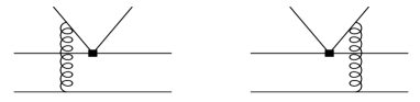
Figure 2.2: Order $\alpha_{s}$ hard spectator interactions.

Figure 2.3: Penguin contractions.

Other calculable corrections to naive factorization are given by penguin contractions (see Fig.2.3), with the insertion of a penguin operator, or the chromomagnetic dipole operator. These contributions introduce complex phases in the hard-scattering kernel which account for perturbative strong-interaction phases, due to the rescattering phase of the penguin loop. This is basically the familiar Bander-Silverman-Soni mechanism for strong phases [35]. However, this is not the only source of strong phases since the vertex corrections in Fig.2.1 also generate imaginary parts. These are correctly included in the QCDF approach.

There is another set of contributions to the decay amplitudes that are completely missing in the generalized factorization formula (2.21). They consist of the processes in which the two quarks inside the B meson annihilate to form the final state partons (see Fig.2.4). These contributions are formally suppressed in the heavy quark limit. However, some of the annihilation topologies related to the corresponding twist-3 light meson LCDA’s are chirally enhanced by the factors $r_{\chi}$, and for realistic b-quark masses the suppression $\Lambda_{QCD}/m_{b}$ might not be sufficient to neglect these terms. Unfortunately, logarithmic end-point divergencies do not cancel properly within these terms, leading to the appearance of non-factorizable contributions. Some power suppressed terms contributing to hard-spectator graphs also suffer from this disease. These corrections constitute one of the weak points of QCDF at the phenomenological level. We shall come back to this issue later.

Figure 2.4: Weak annihilation contributions.

The final formula for the amplitudes in QCDF is then exactly the same one as Eq.(2.21), except that the coefficients $a_{i}^{\rm eff}$ are not phenomenological parameters anymore, but are completely calculable in perturbation theory. Moreover, one should add the hard-spectator and annihilation contributions that do not fit in the scheme of Eq.(2.21). The final formulae for the amplitudes at order $\alpha_{s}$ will be given in the following section. An important observation is that naive factorization arises formally from this picture as a prediction of QCD at leading order in $\alpha_{s}$ and $\Lambda_{QCD}/m_{b}$. This justifies mathematically the phenomenological successes and limitations of the naive factorization approach. Moreover, beyond leading order in $\alpha_{s}$ the scale and scheme dependences are correctly cancelled between the Wilson coefficients and the matrix elements. A proof of factorization in QCDF has however been only given at order $\alpha_{s}^{2}$ for heavy-light final states [23], and the all order proof is not straightforward. Towards this end a more systematic formalism based on an effective lagrangian (SCET) is more useful [33].

The significant property of the factorization approach in phenomenology is the fact that the non perturbative quantities that appear in the formulae for the amplitudes are much simpler objects than the original hadronic matrix elements. These simpler objects are either related to universal properties of a single meson state, as is the case for the light-cone distribution amplitudes, or describe the $B\to$ meson transition matrix element of a local current, parameterized by a form factor. These are objects that appear in many different decay amplitudes, and can therefore be extracted from data and used to make predictions on other modes. Moreover, one can also use QCD sum-rule techniques to study them, or extract them from the lattice. Factorization is a consequence of the fact that in the heavy quark limit only hard interactions between the ‘$B\to$ meson’ and the ‘ejected-meson’ systems are relevant.

2.1.4 $B\to M_{1}M_{2}$ amplitudes in QCD Factorization

Here we collect the relevant formulae for the $B\to M_{1}M_{2}$ amplitudes in QCD Factorization according to [27, 28]. The amplitudes are given as matrix elements of the transition operators $\mathcal{T}_{A}^{p}$ and $\mathcal{T}_{B}^{p}$,

$$\langle M_{1}M_{2}|{\cal H}_{\rm eff}|\bar{B}\rangle=\sum_{p=u,c}\lambda_{p}^{\scriptscriptstyle(D)*}\langle M_{1}M_{2}|\mathcal{T}_{A}^{p}+\mathcal{T}_{B}^{p}|\bar{B}\rangle.$$ (2.43)

The transition operator $\mathcal{T}_{A}^{p}$ contains the contribution from the leading order tree diagrams, and the next-to-leading order vertex corrections, penguin and hard spectator-scattering. It can be written as

$${\cal T}_{A}^{p} = \delta_{pu}\,\alpha_{1}(M_{1}M_{2})\,A([\bar{q}_{s}u][\bar{u}D])+\delta_{pu}\,\alpha_{2}(M_{1}M_{2})\,A([\bar{q}_{s}D][\bar{u}u])$$

$$+ \alpha_{3}^{p}(M_{1}M_{2})\,\sum_{q}A([\bar{q}_{s}D][\bar{q}q])+\alpha_{4}^{p}(M_{1}M_{2})\,\sum_{q}A([\bar{q}_{s}q][\bar{q}D])$$

$$+ \alpha_{3,\rm EW}^{p}(M_{1}M_{2})\,\sum_{q}\frac{3}{2}\,e_{q}\,A([\bar{q}_{s}D][\bar{q}q])+\alpha_{4,\rm EW}^{p}(M_{1}M_{2})\,\sum_{q}\frac{3}{2}\,e_{q}\,A([\bar{q}_{s}q][\bar{q}D])\,,$$

where the operators $A([\cdots][\cdots])$ and their matrix elements are the same as introduced above. Notice that this is basically the same formula (2.21). The sums extend over $q=u,d,s$ and $\bar{q}_{s}$ is the spectator antiquark. The $\alpha_{i}^{p}$ coefficients are given by

$$\alpha_{1}(M_{1}M_{2}) = a_{1}(M_{1}M_{2})\,,$$

$$\alpha_{2}(M_{1}M_{2}) = a_{2}(M_{1}M_{2})\,,$$

$$\alpha_{3}^{p}(M_{1}M_{2}) = \left\{\begin{array}[]{cl}a_{3}^{p}(M_{1}M_{2})-a_{5}^{p}(M_{1}M_{2})\,;&\quad\mbox{if~{}}M_{1}M_{2}=PP,\,VP\,,\\ a_{3}^{p}(M_{1}M_{2})+a_{5}^{p}(M_{1}M_{2})\,;&\quad\mbox{if~{}}M_{1}M_{2}=PV,\,VV\,,\end{array}\right.$$ (2.47)

$$\alpha_{4}^{p}(M_{1}M_{2}) = \left\{\begin{array}[]{cl}a_{4}^{p}(M_{1}M_{2})+r_{\chi}^{M_{2}}\,a_{6}^{p}(M_{1}M_{2})\,;&\quad\mbox{if~{}}M_{1}M_{2}=PP,\,PV\,,\\[2.84544pt] a_{4}^{p}(M_{1}M_{2})-r_{\chi}^{M_{2}}\,a_{6}^{p}(M_{1}M_{2})\,;&\quad\mbox{if~{}}M_{1}M_{2}=VP,\,VV\,,\end{array}\right.$$ (2.50)

$$\alpha_{3,\rm EW}^{p}(M_{1}M_{2}) = \left\{\begin{array}[]{cl}a_{9}^{p}(M_{1}M_{2})-a_{7}^{p}(M_{1}M_{2})\,;&\quad\mbox{if~{}}M_{1}M_{2}=PP,\,VP\,,\\[2.84544pt] a_{9}^{p}(M_{1}M_{2})+a_{7}^{p}(M_{1}M_{2})\,;&\quad\mbox{if~{}}M_{1}M_{2}=PV,\,VV\,,\end{array}\right.$$ (2.53)

$$\alpha_{4,\rm EW}^{p}(M_{1}M_{2}) = \left\{\begin{array}[]{cl}a_{10}^{p}(M_{1}M_{2})+r_{\chi}^{M_{2}}\,a_{8}^{p}(M_{1}M_{2})\,;&\quad\mbox{if~{}}M_{1}M_{2}=PP,\,PV\,,\\[2.84544pt] a_{10}^{p}(M_{1}M_{2})-r_{\chi}^{M_{2}}\,a_{8}^{p}(M_{1}M_{2})\,;&\quad\mbox{if~{}}M_{1}M_{2}=VP,\,VV\,.\end{array}\right.$$ (2.56)

where, at next-to-leading order in $\alpha_{s}$, the coefficients $a_{i}^{p}$ have the following general form

$$a_{i}^{p}(M_{1}M_{2}) = \left(C_{i}+\frac{C_{i\pm 1}}{N_{c}}\right)N_{i}(M_{2})$$ (2.57)

$$+\,\frac{C_{i\pm 1}}{N_{c}}\,\frac{C_{F}\alpha_{s}}{4\pi}\left[V_{i}(M_{2})+\frac{4\pi^{2}}{N_{c}}\,H_{i}(M_{1}M_{2})\right]+P_{i}^{p}(M_{2})\,.$$

The coefficient $N_{i}(M_{2})$ is the leading order term, $V_{i}(M_{2})$ contains the vertex terms, the $P_{i}^{p}$ are the penguin terms and the $H_{i}(M_{1}M_{2})$ are the hard spectator terms. The expressions in terms of meson distribution amplitudes and the various hard-scattering functions can be found in [27, 28].

The transition operator $\mathcal{T}_{B}^{p}$ contains the contributions from weak annihilation and is written as

$${\cal T}_{B}^{p} = \delta_{pu}\,b_{1}(M_{1}M_{2})\,\sum_{q^{\prime}}B([\bar{u}q^{\prime}][\bar{q}^{\prime}u][\bar{D}b])+\delta_{pu}\,b_{2}(M_{1}M_{2})\,\sum_{q^{\prime}}B([\bar{u}q^{\prime}][\bar{q}^{\prime}D][\bar{u}b])$$

$$\!\!+ b_{3}^{p}(M_{1}M_{2})\,\sum_{q,q^{\prime}}B([\bar{q}q^{\prime}][\bar{q}^{\prime}D][\bar{q}b])+b_{4}^{p}(M_{1}M_{2})\,\sum_{q,q^{\prime}}B([\bar{q}q^{\prime}][\bar{q}^{\prime}q][\bar{D}b])$$

$$\!\!\!+ b_{3,\rm EW}^{p}(M_{1}M_{2})\,\sum_{q,q^{\prime}}\frac{3}{2}\,e_{q}\,B([\bar{q}q^{\prime}][\bar{q}^{\prime}D][\bar{q}b])+b_{4,\rm EW}^{p}(M_{1}M_{2})\,\sum_{q,q^{\prime}}\frac{3}{2}\,e_{q}\,B([\bar{q}q^{\prime}][\bar{q}^{\prime}q][\bar{D}b])$$

$$\!\!\!+ \delta_{pu}\,b_{S1}(M_{1}M_{2})\,\sum_{q^{\prime}}B([\bar{u}u][\bar{q}^{\prime}\!q^{\prime}][\bar{D}b])+\delta_{pu}\,b_{S2}(M_{1}M_{2})\,\sum_{q^{\prime}}B([\bar{u}D][\bar{q}^{\prime}\!q^{\prime}][\bar{u}b])$$

$$\!\!\!+ b_{S3}^{p}(M_{1}M_{2})\,\sum_{q,q^{\prime}}B([\bar{q}D][\bar{q}^{\prime}\!q^{\prime}][\bar{q}b])+b_{S4}^{p}(M_{1}M_{2})\,\sum_{q,q^{\prime}}B([\bar{q}q][\bar{q}^{\prime}\!q^{\prime}][\bar{D}b])$$

$$\!\!\!+ b_{S3,\rm EW}^{p}(M_{1}M_{2})\,\sum_{q,q^{\prime}}\frac{3}{2}\,e_{q}\,B([\bar{q}D][\bar{q}^{\prime}\!q^{\prime}][\bar{q}b])+b_{S4,\rm EW}^{p}(M_{1}M_{2})\,\sum_{q,q^{\prime}}\frac{3}{2}\,e_{q}\,B([\bar{q}q][\bar{q}^{\prime}\!q^{\prime}][\bar{D}b])\,,$$

where the matrix elements of the operators $B([\cdots][\cdots][\cdots])$ are given by

$$\langle M_{1}M_{2}|B([\ldots][\ldots]][\ldots])|\bar{B}_{q}\rangle\equiv c\,B_{\scriptscriptstyle M_{1}M_{2}}\,,\quad\mbox{with}\quad B_{\scriptscriptstyle M_{1}M_{2}}=\pm i\,\frac{G_{F}}{\sqrt{2}}\,f_{B_{q}}f_{M_{1}}f_{M_{2}}\,,$$ (2.59)

whenever the quark flavors of the three brackets match those of $M_{1}$, $M_{2}$, and $\bar{B}_{q}$. The constant $c$ is the same as for the $A$ operators. The upper sign applies when both mesons are pseudoscalar and the lower sign otherwise.

The coefficients with the subscript ‘S’ contribute only to final states containing flavor-singlet mesons or neutral vector mesons. The expressions for the $b_{i}$ coefficients can be found in [27, 28].

Up to this point it useful to look closely at the contributions that are dangerous in QCDF, mainly the hard-spectator and the annihilation terms with twist-3 LCDA insertion. The hard-spectator terms receive a contribution of this form:

$$H(M_{1}M_{2})\supset\frac{B_{\scriptscriptstyle M_{1}M_{2}}}{A_{\scriptscriptstyle M_{1}M_{2}}}\frac{m_{B}}{\lambda_{B}}\int_{0}^{1}\!dx\,\int_{0}^{1}\!dy\ r_{\chi}^{\scriptscriptstyle M_{1}}\frac{\Phi_{M_{2}}(x)\Phi_{m_{1}}(y)}{x\bar{y}}\ \propto\int_{0}^{1}\frac{dy}{\bar{y}}\Phi_{m_{1}}(y)$$ (2.60)

where $\lambda_{B}$ is defined in (2.42). This contribution is formally suppressed in the heavy quark limit, but the presence of the chiral factor $r_{\chi}^{\scriptscriptstyle M_{1}}$ makes it phenomenologically important. Moreover, as can be seen by plugging in $\Phi_{p}(y)=1$ or $\Phi_{v}(y)$ as given in (2.38), there is a divergence coming from the region $y\sim 1$. This infrared divergence is a manifestation of the fact that factorization does not hold in this case.

It is customary to extract this divergence defining a parameter $X_{H}^{M_{1}}\equiv\int_{0}^{1}dy/\bar{y}$ such that

$$\int_{0}^{1}\frac{dy}{\bar{y}}\Phi_{m_{1}}(y)=\Phi_{m_{1}}(1)X_{H}^{M_{1}}+\int_{0}^{1}\frac{dy}{\bar{y}}\left[\Phi_{m_{1}}(y)-\Phi_{m_{1}}(1)\right]$$ (2.61)

Because this divergence is associated with a soft interaction of the ejected meson with the spectator quark, the divergence arises specifically from the region $\bar{y}\sim\Lambda_{QCD}/m_{b}$, and therefore one expects that $X_{H}^{M}\sim\log(m_{b}/\Lambda_{QCD})$ with an a priori arbitrary strong phase. The choice for the values of $X_{H}^{M}$ introduces an unavoidable model dependence in the predictions.

Consider now the chirally enhanced contributions to the annihilation terms with 3-twist LCDA insertions. For illustration we take the coefficient $b_{1}$ in Eq.(LABEL:Bops), which contains a term

$$b_{1}(M_{1}M_{2})\supset\frac{C_{F}}{N^{2}}C_{1}\pi\alpha_{s}\int_{0}^{1}\!dx\int_{0}^{1}\!dy\ r_{\chi}^{M_{1}}r_{\chi}^{M_{2}}\Phi_{m_{2}}(x)\Phi_{m_{1}}(y)\frac{2}{\bar{x}y}\ .$$ (2.62)

This contribution is again infrared divergent from the regions $\,y,\bar{x}\sim\Lambda_{QCD}/m_{b}\,$. As before, the divergencies are parameterized by the quantities $X_{A}^{M_{1}}$ and $X_{A}^{M_{2}}$ that introduce an unavoidable model dependence. The rest of the coefficients in Eq.(LABEL:Bops) are also affected by these divergencies, and signal the breakdown of factorization.

A way to get around these inconveniences at the phenomenological level was proposed in [36] and used later in [37, 38, 39, 40]. The basic idea is that the so called GIM penguin is in many cases free from these divergencies when computed in QCDF, since it is dominated by short-distance physics. This quantity (that we call $\Delta$), is given generically by

$$\Delta_{\scriptscriptstyle M_{1}M_{2}}=A_{\scriptscriptstyle M_{1}M_{2}}\frac{C_{F}\alpha_{s}}{4\pi N}C_{1}\big{[}\bar{G}(m_{c}^{2}/m_{b}^{2})-\bar{G}(0)\big{]}$$ (2.63)

where $\bar{G}(x)$ are penguin functions. Using this infrared safe theoretical quantity together with data and some SU(3) relations, predictions can be made safer and more precise. This will be discussed in Chapters 5 and 6.

2.2 Symmetries

It should be clear by now that the strong interaction dynamics inside the matrix elements is a very big deal. An impressive progress has been observed in the past decade concerning the idea of factorization in B physics, but direct computations of amplitudes from QCD still suffer from two diseases. First, the computations involve a great amount of work, combining tedious perturbative calculations, lattice simulations and other technicalities. Second, the theoretical validity of such approaches at the phenomenological level is threatened by corrections to the heavy quark limit and by potentially non-factorizable long-distance leading effects, like the case of the long-distance charm loop issue (“charming penguins”) [41, 42, 43, 44, 45].

Fortunately there is a complementary approach to B-decay phenomenology that relies on the approximate flavor symmetries of QCD, and incorporates naturally all the hadronic information that cannot be extracted from first principles. The drawback is of course the uncontrollable symmetry breaking effects, and the fact that only certain relations between observables can be obtained. However, these relations have been very useful in order to extract CKM parameters from experimental data on non-leptonic decays. In this section we review schematically how this flavor symmetry relations are obtained.

Consider the lagrangian of massless QCD with $n_{f}$ quark flavors

$$\mathcal{L}_{QCD}=-\frac{1}{4}F^{a\,\mu\nu}F_{\mu\nu}^{a}+i\,\sum_{k=1}^{n_{f}}\,\bar{q}_{k}\,D/\ q_{k}$$ (2.64)

This lagrangian has global symmetry $SU(n_{f})_{V}\otimes SU(n_{f})_{A}\otimes U(1)_{V}\otimes U(1)_{A}$. For example, for $n_{f}=2$ (u & d quarks), this symmetry is expected to hold with good precision due to the smallness of $m_{u}$ and $m_{d}$. The first term $SU(2)_{V}$ is isospin, and it is seen to be a good symmetry. The second term $SU(2)_{A}$ is not observed as a symmetry of nature, because this symmetry is spontaneously broken by the quark condensate $\langle\bar{q}q\rangle$, giving rise to goldstone bosons that we observe as pions. The third term $U(1)_{V}$ is nothing but baryon number conservation, which is obviously observed. The last term $U(1)_{A}$ led originally to the so called $U(1)$-problem [46], but later it was found that in fact this symmetry is broken by instantons [47]. So it is clear that, at least for two flavors, the approximate global symmetry is well understood and under control. In the case of isospin, the symmetry breaking effects are expected at the level of a few percent.

For $n_{f}=3$ flavors, the flavor SU(3) symmetry is not so exact as isospin, since the strange quark mass is high compared with $m_{u,d}$. However, the main feature of a SU(3) flavor symmetry is phenomenologically realized: we observe the $(\pi,K,\eta)$ pseudoscalar octet, and the power of group theory can be applied to SU(3) in the same way as for isospin. The predictions, nonetheless, will be affected by symmetries breaking uncertainties of $\sim 20\%$, or maybe higher [48].

2.2.1 The Wigner-Eckart Theorem

The Wigner-Eckart theorem is the mathematical prescription to extract the maximal advantage from a symmetry group in a quantum mechanical system. Although the Wigner-Eckart theorem can be formulated with total generality, we just quote here the theorem for $SU(2)$, as used in elementary quantum mechanics when adding angular momenta. In the next section we will use this theorem to write a simple flavor symmetry relation between $B\to\pi K$ amplitudes.

Given a symmetry group of the system under consideration, any operator can in general be decomposed in terms of irreducible tensor operators, defined as operators that transform as tensors of a given rank under the symmetry group. In the case of SU(2), an irreducible rank-$k$ operator is a $(2k+1)$-tuple of operators $Q^{(k)}_{q}$ ($q=-k,-k+1,\dots,k$), satisfying the proper commutation relations,

$$\big{[}J_{\pm},Q^{(k)}_{q}\big{]} = \pm\sqrt{(k\mp q)(k\pm q+1)}\ Q^{(k)}_{q\pm 1}$$

$$\big{[}J_{z},Q^{(k)}_{q}\big{]} = q\ Q^{(k)}_{q}$$ (2.65)

where $J_{\pm}$ are the ladder operators and $J_{z}$ is the Cartan operator of SU(2). The Wigner-Eckart theorem states that the matrix element $\langle\alpha^{\prime};j^{\prime},m^{\prime}|Q^{(k)}_{q}|\alpha;j,m\rangle$ depends on the quantum numbers $m$, $m^{\prime}$ and $q$ only through Clebsch-Gordan coefficients, specifically

$$\langle\alpha^{\prime};j^{\prime},m^{\prime}|Q^{(k)}_{q}|\alpha;j,m\rangle=C(j^{\prime},m^{\prime}|j,k;m,q)\,\langle\alpha^{\prime};j^{\prime}\|Q^{k}\|\alpha;j\rangle\ ,$$ (2.66)

where $C(j^{\prime},m^{\prime}|j,k;m,q)$ is the corresponding Clebsch-Gordan coefficient and the object $\langle\alpha^{\prime};j^{\prime}\|Q^{k}\|\alpha;j\rangle$ is a so called reduced matrix element.

The power of this result is that, although the reduced matrix element cannot be computed from symmetry principles alone, it only depends on the representation on which the objets live in, and therefore one can establish relations between transitions that connect states in the same representations.

2.2.2 A simple example: $B\to\pi K$ Amplitudes

As a simple example of how the Wigner-Eckart theorem applies to flavor symmetries, we derive the famous $B\to\pi K$ amplitude relation [49, 50, 51].

We want to extract the isospin structure of the matrix elements

$$\langle\pi K|{\cal H}_{\rm eff}|B\rangle\ ,$$ (2.67)

where ${\cal H}_{\rm eff}$ is the weak effective Hamiltonian, given in Eqs.(1.27),(1.28) for the SM case. First we decompose the initial and final states in the isospin basis. $(B^{0},B^{+})$ and $(K^{0},K^{+})$ are isospin doublets, and $(\pi^{-},\pi^{0},\pi^{+})$ is an isospin triplet:

$$|B^{0}\rangle=|1/2,-1/2\rangle\ ,\ |B^{+}\rangle=|1/2,1/2\rangle\ ,$$

$$|K^{0}\rangle=|1/2,-1/2\rangle\ ,\ |K^{+}\rangle=|1/2,1/2\rangle\ ,$$

$$|\pi^{-}\rangle=|1,-1\rangle\ ,\ |\pi^{0}\rangle=|1,0\rangle\ ,\ |\pi^{+}\rangle=|1,1\rangle$$ (2.68)

The isospin decomposition of the $|\pi K\rangle$ states is given by the $(1\otimes\,1/2)$ SU(2) Clebsch-Gordan coefficients,

$$|\pi^{+}K^{0}\rangle=\sqrt{\frac{1}{3}}\ \left|\frac{3}{2}\,,\frac{1}{2}\right\rangle+\sqrt{\frac{2}{3}}\ \left|\frac{1}{2}\,,\frac{1}{2}\right\rangle \!\!\!, |\pi^{-}K^{+}\rangle=\sqrt{\frac{1}{3}}\ \left|\frac{3}{2},-\frac{1}{2}\right\rangle-\sqrt{\frac{2}{3}}\ \left|\frac{1}{2},-\frac{1}{2}\right\rangle\qquad$$

$$|\pi^{0}K^{+}\rangle=\sqrt{\frac{2}{3}}\ \left|\frac{3}{2}\,,\frac{1}{2}\right\rangle-\sqrt{\frac{1}{3}}\ \left|\frac{1}{2}\,,\frac{1}{2}\right\rangle \!\!\!, |\pi^{0}K^{0}\rangle=\sqrt{\frac{2}{3}}\ \left|\frac{3}{2},-\frac{1}{2}\right\rangle+\sqrt{\frac{1}{3}}\ \left|\frac{1}{2},-\frac{1}{2}\right\rangle$$ (2.69)

The next step is to decompose the effective Hamiltonian in terms of irreducible $SU(2)$ tensor operators. But this is easy: the current-current operators $Q_{1,2}^{u}\sim\bar{u}b\bar{s}u$ have components $\Delta I=0$ ad $\Delta I=1$, and so do the electroweak penguin operators $Q_{7,\dots,10}\sim\bar{D}b\sum e_{q}\bar{q}q$; the current-current operators $Q_{1,2}^{c}\sim\bar{c}b\bar{s}c$ and the QCD-penguin operators $Q_{3,\dots,6}\sim\bar{s}b\sum\bar{q}q$ only have $\Delta I=0$ components. Therefore, the effective Hamiltonian can be decomposed as the sum of triplet and singlet tensor operators:

$${\cal H}_{\rm eff}={\cal H}_{\rm eff}^{(1)}\oplus{\cal H}_{\rm eff}^{(0)}$$ (2.70)

Now the matrix elements can be expressed in terms of reduced matrix elements. First we have $\langle 3/2,\pm 1/2|{\cal H}_{\rm eff}^{(0)}|1/2,\pm 1/2\rangle=0$ due to the commutation relations (2.65). For the rest, the Wigner-Eckart theorem implies that

$$\left\langle\frac{3}{2}\,,\pm\frac{1}{2}\,\right|{\cal H}_{\rm eff}^{(1)}\left|\frac{1}{2}\,,\pm\frac{1}{2}\right\rangle \!\!\!=\!\! C\left(\frac{3}{2},\pm\frac{1}{2}\,\Big{|}\,\frac{1}{2},1;\pm\frac{1}{2},0\right)\left\langle\frac{3}{2}\right\|\!{\cal H}_{\rm eff}^{(1)}\!\left\|\frac{1}{2}\right\rangle=\sqrt{\frac{2}{3}}\,\left\langle\frac{3}{2}\right\|\!{\cal H}_{\rm eff}^{(1)}\!\left\|\frac{1}{2}\right\rangle$$

$$\left\langle\frac{1}{2}\,,\pm\frac{1}{2}\,\right|{\cal H}_{\rm eff}^{(1)}\left|\frac{1}{2}\,,\pm\frac{1}{2}\right\rangle \!\!\!=\!\! C\left(\frac{1}{2},\pm\frac{1}{2}\,\Big{|}\,\frac{1}{2},1;\pm\frac{1}{2},0\right)\left\langle\frac{1}{2}\right\|\!{\cal H}_{\rm eff}^{(1)}\!\left\|\frac{1}{2}\right\rangle=\mp\sqrt{\frac{1}{3}}\,\left\langle\frac{1}{2}\right\|\!{\cal H}_{\rm eff}^{(1)}\!\left\|\frac{1}{2}\right\rangle$$

$$\left\langle\frac{1}{2}\,,\pm\frac{1}{2}\,\right|{\cal H}_{\rm eff}^{(0)}\left|\frac{1}{2}\,,\pm\frac{1}{2}\right\rangle \!\!\!=\!\! \left\langle\frac{1}{2}\right\|\!{\cal H}_{\rm eff}^{(0)}\!\left\|\frac{1}{2}\right\rangle$$ (2.71)

It is conventional to define the invariant isospin amplitudes $A_{3/2}$, $A_{1/2}$ and $B_{1/2}$ ,

$$A_{3/2}\equiv\frac{\sqrt{2}}{3}\left\langle\frac{3}{2}\right\|\!{\cal H}_{\rm eff}^{(1)}\!\left\|\frac{1}{2}\right\rangle\ ,\ A_{1/2}\equiv-\frac{\sqrt{2}}{3}\left\langle\frac{1}{2}\right\|\!{\cal H}_{\rm eff}^{(1)}\!\left\|\frac{1}{2}\right\rangle\ ,\ B_{1/2}\equiv\sqrt{\frac{2}{3}}\left\langle\frac{3}{2}\right\|\!{\cal H}_{\rm eff}^{(0)}\!\left\|\frac{1}{2}\right\rangle\ ,$$

so that combining Eqs.(2.69) and (2.71) the amplitudes can be written as

$$A(B^{+}\to\pi^{+}K^{0}) = B_{1/2}+A_{1/2}+A_{3/2}\ ,$$

$$-\sqrt{2}A(B^{+}\to\pi^{0}K^{+}) = B_{1/2}+A_{1/2}-2A_{3/2}\ ,$$

$$-A(B^{0}\to\pi^{-}K^{+}) = B_{1/2}-A_{1/2}-A_{3/2}\ ,$$

$$\sqrt{2}A(B^{0}\to\pi^{0}K^{0}) = B_{1/2}-A_{1/2}+2A_{3/2}\ .$$ (2.72)

From this representation of the amplitudes in terms of reduced matrix elements, the promised $B\to\pi K$ amplitude relation follows:

$$A(B^{+}\!\to\pi^{+}K^{0})-A(B^{0}\!\to\pi^{-}K^{+})+\sqrt{2}A(B^{+}\!\to\pi^{0}K^{+})-\sqrt{2}A(B^{0}\!\to\pi^{0}K^{0})=0$$ (2.73)

2.2.3 Discussion

Following the same procedure as for $B\to\pi K$, it is possible to write other isospin relations. For example, for $B\to\pi\pi\,$, isospin implies

$$A(B^{0}\to\pi^{+}\pi^{-})-\sqrt{2}A(B^{+}\to\pi^{+}\pi^{0})+A(B^{0}\to\pi^{0}\pi^{0})=0\ .$$ (2.74)

Relations arising from SU(3) flavor symmetry are richer, since they mix many other decays that are not just connected by an isospin transformation. The complexity of the group SU(3) with respect to the simplicity of SU(2) is the main reason to avoid a detailed discussion of the technical aspects of the SU(3) analysis here, and the important idea is clear from the example above. The SU(3) Clebsch-Gordan coefficients were collected for the representations of interest by de Swart [52], and the complete SU(3) decomposition of the non-leptonic decay amplitudes of the triplet $(B^{+}_{u},B^{0}_{d},B^{0}_{s})$ into pseudoscalar mesons was given by Grinstein and Lebed [53].

However, the general decomposition of SU(3) amplitudes introduces too many SU(3) invariant amplitudes, so that in order to extract amplitude relations it is often necessary to neglect some of them. But the relative sizes of the reduced matrix elements is a dynamical question, so this process requires a dynamical assumption. Because the language of invariant amplitudes is often obscure in this sense, it is often convenient to use a diagrammatic approach in which the invariant amplitudes are related to flavor-flow topologies (see for example [54]). The amplitudes can then be written in terms of $T$ (tree), $P$ (penguin), $C$ (color suppressed), $E$ (exchange), $A$ (annihilation), $PA$ (penguin annihilation) and electroweak penguins $P_{EW}$ and $P_{EW}^{C}$. Including $b\to s$ transitions doubles the number of parameters, which are usually denoted with primes. Then one can argue that the electroweak penguins are small, and also neglect the contributions $E$, $A$ and $PA$ on the basis of helicity or $f_{B}/m_{B}$-type suppressions [55]. It is, however, far from clear whether these assumptions can be made safely.

An analysis along these lines allows to find flavor symmetry relations that do not rely on any dynamical assumption, like for example [56, 57]

$$A(B^{0}\to K^{0}\pi^{0})-\sqrt{3}A(B^{0}\to K^{0}\eta_{8})=0\ ,$$

$$A(B^{+}\to K^{+}\pi^{0})+\sqrt{2}A(B^{+}\to K^{0}\pi^{+})-\sqrt{3}A(B^{+}\to K^{+}\eta_{8})=0\ ,$$ (2.75)

$$A(B^{0}\to K^{+}\pi^{-})+A(B^{+}\to K^{0}\pi^{+})-\sqrt{6}A(B^{+}\to K^{+}\eta_{8})+\sqrt{6}A(B^{0}\to K^{0}\eta_{8})=0\ .$$

From these relations the isospin $B\to\pi K$ relation (2.73) follows.

Up to this point it not obvious what is the usefulness of these amplitude relations. Indeed, a powerful aspect of flavor symmetry relations is to be able to write relations between observables and not just amplitudes. These relations can be then tested experimentally to probe the size of the SU(3) breaking. Since they are specially sensitive to, for instance, non standard isospin violating contributions, they provide a window for New Physics (see for example [58] for a discussion concerning $B\to\pi K$).

But obtaining relations between observables is not as easy as for the amplitudes. Observables are constructed, roughly, by squaring amplitudes. Therefore, the observables depend on the magnitudes of the invariant amplitudes and also on the strong phases, since there is interference between different invariant amplitudes. For example, in the case of Eq.(2.72), there are two independent CKM parameters entering the decay amplitudes, introducing two weak phases. Each invariant amplitude receives contributions from both weak phases. Up to a global phase, one ends up with five independent strong phases and six independent real amplitudes, to be fitted with four branching ratios and four CP asymmetries [59]. This example shows how a model independent amplitude relation is not sufficient to obtain a model independent observable relation.

Despite the apparent negativity of the discussion above, flavor symmetries have been used in phenomenology with the outcome of very interesting analyses and results, helping to achieve an understanding on B decays that would have not been possible with dynamical approaches alone [59, 60, 61, 62, 63, 64, 65, 66, 67] . Flavor symmetry relations will be used extensively throughout this thesis, specially for $B\to KK$ modes.

Chapter 3 CP Violation in Meson Decays

The fact that nature is not invariant under parity transformations (P) was an early surprise. It was of general common sense to think that one could never tell whether a physical process was being observed through a mirror or directly. Indeed, electromagnetism and strong interactions conserve parity, and in the 1950’s experiments in particle physics were mainly probing the recently developed theory of QED, and the strong interactions of the zoo of hadrons that was just being discovered. The exception was the experiments on $\beta$-decay, that was at that time described by Fermi’s theory. This theory had just been proposed to be universal (e.g, neutron decay and muon decay would have the same coupling constant), and this was the main issue in weak interactions.

However, in 1955 the $\tau$-$\theta$ puzzle raised some confusion. The $\theta^{+}$ would decay in to a CP-even two pion state, and the $\tau^{+}$ into a CP-odd three pion state. Parity invariance necessarily implied that these were two different particles with opposite parity, but the puzzling point was that they were otherwise identical; same charge, same mass, same width. This led to Lee and Yang to point out that while P invariance had been tested in strong and electromagnetic interactions, it had never been verified in weak interactions, and they proposed several experiments. This proposal was taken seriously by Wu’s group, who in 1957 provided first evidence of Parity violation studying the angular distribution of nuclear $\beta$-decay with polarized ${\rm Co}^{60}$ [68]. Their discovery was simultaneously confirmed by Lederman and collaborators with a measurement of the electron asymmetry in pion decay [69]. The discovery of P violation immediately solved the $\tau$-$\theta$ puzzle, a crucial brick in the physics of kaons.

In parallel, the theory of strangeness arose as an explanation to the kaon-hyperon problem. These particles were produced very easily in pairs, but they decayed very slowly. Gell-Mann and Nishijima proposed the existence of a quantum number (strangeness) that was only violated by weak interactions; pair production could then be a strong process, but single decay had to be weak. This was the foundation of flavor physics. An immediate consequence was the existence of two different neutral kaons with opposite strangeness. The separate identity of these two kaons was established very soon by Gell-Mann and Pais in 1955 [70], a discovery that gave birth to the physics of neutral meson mixing.

The oscillation of neutral mesons quickly opened up a chapter in the history of particle physics. The measurement of the oscillation period of neutral kaons through time dependent semileptonic decays allowed the extraction of the tiny mass splitting between the two physical kaons, $\Delta M_{K}/M_{K}\sim 10^{-15}$. Later, studies of regeneration of short-lived kaons in matter revealed an excess of regenerated kaons, a result that had an unexpected origin. In 1964 an experiment by Christenson and collaborators [71] established that both the short-lived and the long-lived components of the neutral kaon system were decaying into a CP even $\pi^{+}\pi^{-}$ mode. The clear interpretation of this discovery was the violation of CP invariance.

Today we have much evidence of CP violating phenomena in kaon and $B_{d}$ meson decays [72]. Measurements of CP asymmetries in $B_{s}$ decays are still compatible with zero at the $2\sigma$ level, but since the experimental prospects are good at Tevatron, and theoretically these asymmetries can be as large as for $B_{d}$ decays, it is safe to say that it will not take long. CP violation has neither been observed in $D$ meson decays, which is very suppressed in the SM. However, at the LHC the sensitivity could reach the 1 per mil for $D$ meson CP asymmetries, making CP violation in the $D$ sector a powerful probe of New Physics.

The SM description of CP violation, the CKM mechanism [73], is successful and economic, involving just one CP violating phase. The fits to the Unitarity Triangle are getting tight [74, 75], and all data is consistent (within experimental and theoretical errors) with a single value for its apex. However, the main reason to believe that there must be sources of CP violation beyond the SM, is the issue of the baryon asymmetry in the universe.

The measurement of baryon asymmetry has recently become accurate (about 5% error) due to the measurements of the fluctuations of the cosmic microwave radiation background. The order of magnitude of the baryon-to-photon ratio is $(n_{B}-n_{\bar{B}})/n_{\gamma}\sim 10^{-10}$. The fact that this asymmetry could have been an initial condition at the big bang is excluded, since any baryon asymmetry present in the early universe would have been diluted by inflation to completely negligible levels. So it is very much accepted that the baryon asymmetry must have a dynamical origin.

The necessary conditions for the dynamical generation of a baryon asymmetry in the universe were studied by Andrei Sakharov in 1967 [76]. There are three main conditions that have to be fulfilled. First, there must exist baryon number violating interactions (this is clear). Second, there must be a departure from thermal equilibrium during a sufficiently long period of time. This is because the baryon number violating interactions must occur in the forward direction predominantly, so there must be an arrow of time. Third, there must be CP violation, since CP invariance would equal the rates of CP-conjugated baryon number violating interactions, thus giving a zero net contribution.

Now, baryon number is broken in the SM by sphalerons at high temperature. The electroweak phase transition, occurring at a temperature $T\sim 100\,{\rm GeV}$, could provide the necessary departure from thermal equilibrium (this is called electroweak baryogenesis). It turns out that this phase transition is not strong enough to produce and maintain the observed baryon asymmetry, but let’s assume it were. Then, the baryon asymmetry can be estimated to be $(n_{B}-n_{\bar{B}})/n_{\gamma}\sim 10^{-2}\cdot J/T^{12}$, where $J$ is the Jarlskog determinant (a measure of CP violation in the SM). For $T\sim 100\,{\rm GeV}$, then $(n_{B}-n_{\bar{B}})/n_{\gamma}\sim 10^{-23}$, so clearly the CP violation in the SM is far too small to account for the observed baryon asymmetry. On the other hand, almost any extension of the SM provides new sources of CP violation, so the search for physics beyond the SM is much in contact with the study of CP violation.

In general, CP violation is the cause that a process and it’s CP-conjugate don’t share the same rights. This means that it is possible to distinguish objectively between CP-conjugated events. In particular, a difference between the decay rate of a given process, $A\to B$, and that of the CP transformed, $\bar{A}\to\bar{B}$, will signal CP violation. This is generally quantified by a so called CP asymmetry, defined as

$$A_{CP}(A\to B)\equiv\frac{\Gamma(A\to B)-\Gamma(\bar{A}\to\bar{B})}{\Gamma(A\to B)+\Gamma(\bar{A}\to\bar{B})}$$ (3.1)

The deviation of any CP asymmetry from zero is a measure of CP violation. In this chapter we will review the general features of CP violation in meson decays and the different types of CP asymmetries that one may encounter.

3.1 Mixing of neutral mesons

The phenomenon of neutral meson mixing is a consequence of flavor violation. Therefore, the mixing is a weak process, and since the mesons themselves are regarded as asymptotic states of the strong Hamiltonian, it is sensible to study the mixing in terms of mesonic degrees of freedom.

The quantum mechanical idea for this phenomenon is very simple. The weak Hamiltonian is not invariant under flavor rotations. This means that flavor eigenstates deviate from mass eigenstates and mix under time evolution. This deviation, as already mentioned, is due to weak effects, and this allows to study the oscillations in a perturbative fashion.

Experimentally, oscillations have been observed in all the low-lying neutral meson systems. The oscillation of neutral kaons was observed for the first time in 1961 [77]. The oscillations of $B_{d}$ mesons was observed in 1987 [78, 79]. The observation of $B_{s}$ and $D$ meson oscillations has taken a much longer time, but they have been observed finally, very recently [80, 81].

In this section we present a general description of particle-antiparticle oscillations in a quantum mechanical approach. We will see in later chapters that the physics of meson oscillations is strongly related to the physics of CP violation.

3.1.1 The effective Hamiltonian

Let $P^{0}$ be a neutral meson carrying an internal additive quantum number $F\neq 0$. For our purposes $F$ is a flavor quantum number. Charge conjugation will change the sign of this quantum number, so the C-conjugate state $\bar{P}^{0}$ is a different neutral meson.

Now, let’s say that $F$ is not conserved, that is, the interaction Hamiltonian contains (weak) breaking terms with $\Delta F\neq 0$. Transitions $P^{0}\leftrightarrow\bar{P}^{0}$ are then possible as a one-step process (through $H_{W}^{\scriptscriptstyle\Delta F=2}$) or through an intermediate state (at second order in $H_{W}^{\scriptscriptstyle\Delta F=1}$). To be specific, we write the full Hamiltonian as

$$H=H_{0}+H_{W}^{\scriptscriptstyle\Delta F=1}+H_{W}^{\scriptscriptstyle\Delta F=2},$$ (3.2)

where $H_{0}$ is the flavor invariant (strong) Hamiltonian. The states $|P^{0}\rangle$ and $|\bar{P}^{0}\rangle$ are then defined as eigenstates of $H_{0}$. As mentioned above, that it actually makes sense to speak about $P^{0}$ and $\bar{P}^{0}$ is due to the fact that $H_{W}$ is weak. On the other hand, the presence of the terms $H_{W}$ will produce $P^{0}-\bar{P}^{0}$ mixing.

Consider now an initial state which is a mixture of a $P^{0}$ and a $\bar{P}^{0}$,

$$|\psi(t=0)\rangle=c\,|P^{0}\rangle+\bar{c}\,|\bar{P}^{0}\rangle.$$ (3.3)

At $t>0$ this state will evolve in two different ways. First, transitions between $P^{0}$ and $\bar{P}^{0}$ will give rise to unitary rotations in the $c-\bar{c}$ space (oscillations). Second, the fact that these mesons can decay into lighter particles will allow the initial state to evolve outside the two meson system:

$$|\psi(t)\rangle=c(t)|P^{0}\rangle+\bar{c}(t)|\bar{P}^{0}\rangle+\sum_{n}c_{n}(t)|n\rangle$$ (3.4)

where $|n\rangle=|\pi\pi\rangle,\,|3\pi\rangle,\,|\pi l\bar{\nu}_{l}\rangle,...$ represents any state of any number of particles which does not violate symmetry requirement –mainly decay modes of the original mesons. We would like to study the time evolution of a general initial state (3.3) inside the 2 dimensional $P^{0}-\bar{P}^{0}$ subspace. To that end we split the full Hamiltonian into a part $H_{0}\equiv H_{\Delta F=0}$ and a part $H_{W}\equiv H_{\Delta F\neq 0}$, $H=H_{0}+H_{W}$, and we follow a time-dependent perturbation theory formalism treating $H_{W}$ as a small correction.

In the interaction picture, the state vectors and operators are defined as follows

$$|\psi(t)\rangle_{I} = e^{iH_{0}t}|\psi(t)\rangle_{S}$$ (3.5)

$$O_{I}(t) = e^{iH_{0}t}O_{S}\,e^{-iH_{0}t}$$ (3.6)

The time evolution in this picture defines the evolution operator $U_{I}(t)$ through

$$|\psi(t)\rangle_{I}=U_{I}(t)|\psi(0)\rangle,$$ (3.7)

so that the evolution of the coefficients $c(t)$ and $\bar{c}(t)$ is given exactly by

$$\left\{\begin{array}[]{l}c(t)=\langle P^{0}|U_{I}(t)|\psi(0)\rangle=c\,\langle P^{0}|U_{I}(t)|P^{0}\rangle+\bar{c}\,\langle P^{0}|U_{I}(t)|\bar{P}^{0}\rangle\\ \bar{c}(t)=\langle\bar{P}^{0}|U_{I}(t)|\psi(0)\rangle=c\,\langle\bar{P}^{0}|U_{I}(t)|P^{0}\rangle+\bar{c}\,\langle\bar{P}^{0}|U_{I}(t)|\bar{P}^{0}\rangle\end{array}\right.$$ (3.8)

The unitary operator $U_{I}(t)$ verifies the Schrödinger equation

$$i\partial_{t}U_{I}(t)=H_{W}(t)\cdot U_{I}(t),$$ (3.9)

where $H_{W}(t)\equiv(H_{W})_{I}$. The solution of (3.9) with initial condition $U_{I}(0)=1$ can be computed perturbatively

$$U_{I}(t)=1-i\int_{0}^{t}\!dt^{\prime}H_{W}(t^{\prime})-\int_{0}^{t}\!dt^{\prime}\int_{0}^{t^{\prime\prime}}\!dt^{\prime}H_{W}(t^{\prime})H_{W}(t^{\prime\prime})+\cdots$$ (3.10)

We are interested only in the time evolution of the projection of the full state $|\psi(t)\rangle$ on the two-dimensional subspace of the $P^{0}-\bar{P}^{0}$ system. This evolution is NOT unitary, and effectively is described by a Schrödinger-like equation:

$$i\partial_{t}\left(\begin{array}[]{c}\!\!c(t)\!\!\\ \!\!\bar{c}(t)\!\!\end{array}\right)=\mathcal{H}_{\rm eff}\left(\begin{array}[]{c}\!\!c(t)\!\!\\ \!\!\bar{c}(t)\!\!\end{array}\right)\equiv\left(\begin{array}[]{cc}\langle P^{0}|\hat{\mathcal{H}}_{\rm eff}|P^{0}\rangle&\langle P^{0}|\hat{\mathcal{H}}_{\rm eff}|\bar{P}^{0}\rangle\\ \langle\bar{P}^{0}|\hat{\mathcal{H}}_{\rm eff}|P^{0}\rangle&\langle\bar{P}^{0}|\hat{\mathcal{H}}_{\rm eff}|\bar{P}^{0}\rangle\end{array}\right)\left(\begin{array}[]{c}\!\!c(t)\!\!\\ \!\!\bar{c}(t)\!\!\end{array}\right)$$ (3.11)

This is an effective description valid at time scales much larger than the typical strong interaction scale, and it’s called the Wigner-Weisskopf approximation [82]. In particular, the effective Hamiltonian $\mathcal{H}_{\rm eff}$ will not be hermitian.

By introducing (3.8) in (3.11), and using (3.10), we find an equation for $\mathcal{H}_{\rm eff}$:

$$\langle a|H_{W}(t)|b\rangle-i\langle a|H_{W}(t)\int_{0}^{t}dt^{\prime}H_{W}(t^{\prime})|b\rangle+\cdots\hskip 113.81102pt$$

$$=\langle a|\mathcal{H}_{\rm eff}|b\rangle-i\langle a|\sum_{m}\mathcal{H}_{\rm eff}|m\rangle\langle m|\int_{0}^{t}dt^{\prime}H_{W}(t^{\prime})|b\rangle+\cdots$$ (3.12)

where $a,b,m\in\{P^{0},\bar{P}^{0}\}$. We can solve this equation order by order in $H_{W}$. For our purpose here it will be enough to stop at second order:

$$\mathcal{H}_{\rm eff}=H_{W}+\sum_{n}H_{W}|n\rangle\langle n|H_{W}\left(\mathcal{P}\frac{1}{m_{P}-E_{n}+i\epsilon}-i\pi\delta(m_{P}-E_{n})\right)+\cdots$$ (3.13)

Here, $\mathcal{P}$ stands for the principal part prescription, and the sum runs over all intermediate states $n$. $m_{P}$ and $E_{n}$ are the energies in the center of mass frame defined as $H_{0}|P^{0}\rangle=m_{P}|P^{0}\rangle$, $H_{0}|\bar{P}^{0}\rangle=m_{P}|\bar{P}^{0}\rangle$ and $H_{0}|n\rangle=E_{n}|n\rangle$.

Up to this point we introduce two hermitian operators $M$ and $\Gamma$ defined as

$$M \equiv \frac{1}{2}(\mathcal{H}_{\rm eff}+\mathcal{H}_{\rm eff}^{\dagger})$$

$$\Gamma \equiv i(\mathcal{H}_{\rm eff}-\mathcal{H}_{\rm eff}^{\dagger}).$$ (3.14)

By inversion of (3.14) we can write the effective Hamiltonian in terms of $M$ and $\Gamma$,

$$\mathcal{H}_{\rm eff}=M-\frac{i}{2}\Gamma=\left(\begin{array}[]{cc}M_{11}-\frac{i}{2}\Gamma_{11}&M_{12}-\frac{i}{2}\Gamma_{12}\\[2.0pt] M_{21}-\frac{i}{2}\Gamma_{21}&M_{22}-\frac{i}{2}\Gamma_{22}\end{array}\right)$$ (3.15)

and the explicit matrix elements for $M$ and $\Gamma$ can be read off from equations (3.13) and (3.14),

$$M_{11} = m_{P}+\sum_{n}\mathcal{P}\frac{|\langle n|H_{W}^{\scriptscriptstyle\Delta F=1}|P^{0}\rangle|^{2}}{m_{P}-E_{n}}$$

$$M_{22} = m_{P}+\sum_{n}\mathcal{P}\frac{|\langle n|H_{W}^{\scriptscriptstyle\Delta F=1}|\bar{P}^{0}\rangle|^{2}}{m_{P}-E_{n}}$$

$$M_{12} = M_{21}^{*}=\langle P^{0}|H_{W}^{\scriptscriptstyle\Delta F=2}|\bar{P}^{0}\rangle+\sum_{n}\mathcal{P}\frac{\langle P^{0}|H_{W}^{\scriptscriptstyle\Delta F=1}|n\rangle\langle n|H_{W}^{\scriptscriptstyle\Delta F=1}|\bar{P}^{0}\rangle}{m_{P}-E_{n}}$$

$$\Gamma_{11} = 2\pi\sum_{n}\delta(m_{P}-E_{n})|\langle n|H_{W}^{\scriptscriptstyle\Delta F=1}|P^{0}\rangle|^{2}$$

$$\Gamma_{22} = 2\pi\sum_{n}\delta(m_{P}-E_{n})|\langle n|H_{W}^{\scriptscriptstyle\Delta F=1}|\bar{P}^{0}\rangle|^{2}$$

$$\Gamma_{12} = \Gamma_{21}^{*}=2\pi\sum_{n}\delta(m_{P}-E_{n})\langle P^{0}|H_{W}^{\scriptscriptstyle\Delta F=1}|n\rangle\langle n|H_{W}^{\scriptscriptstyle\Delta F=1}|\bar{P}^{0}\rangle$$ (3.16)

Assuming CPT as a symmetry of $H_{W}$ leads to the following relations

$$M_{11}=M_{22}\equiv M_{0}\ ,\quad\Gamma_{11}=\Gamma_{22}\equiv\Gamma_{0}.$$ (3.17)

3.1.2 Mass eigenstates: Diagonalizing the effective Hamiltonian

The mesons $P^{0}$ and $\bar{P}^{0}$ are charge-conjugated states, and hence they differ only by the sign of their internal additive quantum numbers. They are eigenstates of $H_{0}$, which conserves such quantum numbers, but not of $H_{W}$. Therefore these are not physical states (or mass eigenstates) with the corresponding consequence of mixing and decay. There is a feature, however, that decouples the process of mixing with that of decay, and allows to treat them separately: oscillations are unitary in the two dimensional subspace, but decay is not. A new basis $\{P_{L},P_{H}\}$ which diagonalizes $\mathcal{H}_{\rm eff}$ defines two fields that do not oscillate, just decay. Of course the question arises of whether $M$ and $\Gamma$ can be diagonalized simultaneously. In general they cannot, so no unitary transformation can diagonalize $\mathcal{H}_{\rm eff}$, and the states $\{P_{L},P_{H}\}$ will not be orthogonal. The formalism to deal with this issue was developed by T.D. Lee and L. Wolfenstein in 1965 [83].

To simplify the notation, we parameterize the effective Hamiltonian in terms of three complex numbers, $A$, $B$ and $r$:

$$\mathcal{H}_{\rm eff}=\left(\begin{array}[]{cc}A&B/r\\ rB&A\end{array}\right)$$ (3.18)

where CPT has been assumed through (3.17). By comparing (3.18) with (3.15) we see that

$$A = M_{0}-\frac{i}{2}\Gamma_{0}$$ (3.19)

$$B = \sqrt{(M_{12}-\frac{i}{2}\Gamma_{12})(M_{12}^{*}-\frac{i}{2}\Gamma_{12}^{*})}$$ (3.20)

$$r = \sqrt{\frac{M_{12}^{*}-\frac{i}{2}\Gamma_{12}^{*}}{M_{12}-\frac{i}{2}\Gamma_{12}}}$$ (3.21)

The eigenvalues and eigenstates are then

$$\mathcal{H}_{\rm eff}|P_{L}\rangle = (A+B)|P_{L}\rangle\equiv\big{(}M_{L}-\frac{i}{2}\Gamma_{L}\big{)}|P_{L}\rangle$$

$$\mathcal{H}_{\rm eff}|P_{H}\rangle = (A-B)|P_{H}\rangle\equiv\big{(}M_{H}-\frac{i}{2}\Gamma_{H}\big{)}|P_{H}\rangle$$ (3.22)

$$|P_{L}\rangle = \frac{1}{\sqrt{1+|r|^{2}}}\big{(}|P^{0}\rangle+r|\bar{P}^{0}\rangle\big{)}$$

$$|P_{H}\rangle = \frac{1}{\sqrt{1+|r|^{2}}}\big{(}|P^{0}\rangle-r|\bar{P}^{0}\rangle\big{)}$$ (3.23)

As mentioned above, the mass eigenstates $\{P_{L},P_{H}\}$ are not necessarily orthogonal. This can be easily seen by inspection of (3.23), since the non-hermiticity of $\mathcal{H}_{\rm eff}$ allows $|r|\neq 1$. However, the amount of non-orthogonality is constrained by the exclusive widths of $P_{L}$ and $P_{H}$. The proof goes as follows. Consider the braket

$$\langle P_{H}|\Gamma|P_{L}\rangle=\langle P_{H}|i(\mathcal{H}_{\rm eff}-\mathcal{H}_{\rm eff}^{\dagger})|P_{L}\rangle=\Big{[}\frac{1}{2}(\Gamma_{L}+\Gamma_{H})+i(M_{L}-M_{H})\Big{]}\langle P_{H}|P_{L}\rangle$$ (3.24)

This quantity can be calculated from (3.16),

$$\langle P_{H}|\Gamma|P_{L}\rangle=2\pi\sum_{f}\delta(m_{P}-E_{f})\langle f|H|P_{H}\rangle^{*}\langle f|H|P_{L}\rangle\,.$$ (3.25)

We denote $\langle f|H|P\rangle\equiv\Gamma^{f}$. Then by means of the Schwartz inequality, $\left|\langle P_{H}|\Gamma|P_{L}\rangle\right|^{2}\leq\sum_{f}\Gamma_{L}^{f}\Gamma_{H}^{f}$, we find that

$$|\langle P_{H}|P_{L}\rangle|\leq\sqrt{\frac{\sum_{f}4\Gamma_{L}^{f}\Gamma_{H}^{f}}{(\Gamma_{L}+\Gamma_{H})^{2}+4(M_{L}-M_{H})^{2}}}\ \ .$$ (3.26)

The equation (3.26) is called the Bell-Steinberger inequality. Note that if $H_{W}^{\scriptscriptstyle\Delta F=1}=0$, then the states do not decay, only mix (if $H_{W}^{\scriptscriptstyle\Delta F=2}\neq 0$, of course). Therefore $\Gamma^{f}=0$, but still $M_{L}\neq M_{H}$, so $\langle P_{H}|P_{L}\rangle=0$. This would correspond to a conventional unitary mixing.

3.1.3 Time evolution

We denote by $|P(t)\rangle$ the state at time $t$ that at $t=0$ was a pure $|P\rangle$. The time evolution of the flavor states $P^{0},\bar{P^{0}}$ is complicated because of the mixing, in the sense that the states $|P^{0}(t)\rangle$ and $|\bar{P}^{0}(t)\rangle$ will be superpositions of $P^{0}$ and $\bar{P^{0}}$ at $t>0$. However, the time evolution of the mass eigenstates is quite simple since they diagonalize the effective Hamiltonian. From (3.11) and (3.22) we find the usual time evolution for decaying stationary states:

$$|P_{L,H}(t)\rangle=e^{-iM_{L,H}t}e^{-\frac{1}{2}\Gamma_{L,H}t}|P_{L,H}\rangle$$ (3.27)

By inversion of (3.23) we can find the time evolution of the states $P^{0},\bar{P^{0}}$,

$$|P^{0}(t)\rangle = g_{+}(t)|P^{0}\rangle+rg_{-}(t)|\bar{P}^{0}\rangle$$

$$|\bar{P}^{0}(t)\rangle = g_{+}(t)|\bar{P}^{0}\rangle+\frac{1}{r}g_{-}(t)|P^{0}\rangle$$ (3.28)

where, to avoid cumbersome expressions, we have defined

$$g_{\pm}(t)=\frac{1}{2}e^{-iM_{L}t}e^{-\frac{1}{2}\Gamma_{L}t}\big{(}1\pm e^{-i\Delta\!M\,t}e^{\frac{1}{2}\Delta\Gamma\,t}\big{)}$$ (3.29)

and

$$\Delta M\equiv M_{H}-M_{L},\quad\Delta\Gamma\equiv\Gamma_{L}-\Gamma_{H}.$$ (3.30)

We are interested in the time evolution of observables such as branching ratios, decay rates, and CP asymmetries. We define $A_{f}$ and $\bar{A}_{f}$ as the amplitudes for the decay of $P^{0}$ and $\bar{P}^{0}$ into a final state f , i.e.,

$$A_{f}\equiv\langle f|H_{W}^{\scriptscriptstyle\Delta F=1}|P^{0}\rangle\ ,\quad\bar{A}_{f}\equiv\langle f|H_{W}^{\scriptscriptstyle\Delta F=1}|\bar{P}^{0}\rangle$$ (3.31)

The decay rates are proportional to the square of the time dependent decay amplitudes, the proportionality factor given by a phase space factor $f_{\scriptscriptstyle\textrm{PS}}$ (see the Appendix at the end of this chapter). From (3.98), (3.28) and (3.31) we find the following master equations for the time dependent decay rates,

$$\Gamma(P^{0}(t)\!\rightarrow\!f) \!\!\!\!= \!\!\!\!\frac{1}{4}\,f_{\scriptscriptstyle\textrm{PS}}\,e^{-\Gamma_{L}t}\,|A_{f}|^{2}\Big{[}K_{+}(t)+K_{-}(t)\,|\lambda_{f}|^{2}+2\textrm{Re}\big{(}L(t)\,\lambda_{f}\big{)}\Big{]}$$ (3.32)

$$\Gamma(\bar{P}^{0}(t)\!\rightarrow\!f) \!\!\!\!= \!\!\!\!\frac{1}{4}\,f_{\scriptscriptstyle\textrm{PS}}\,e^{-\Gamma_{L}t}\,|A_{f}|^{2}\left|\frac{1}{r}\right|^{2}\Big{[}K_{+}(t)\,|\lambda_{f}|^{2}+K_{-}(t)+2\textrm{Re}\big{(}L(t)\,\lambda_{f}^{*}\big{)}\Big{]}$$ (3.33)

where

$$K_{\pm}(t) \equiv 1+e^{\Delta\Gamma t}\pm 2e^{\frac{1}{2}\Delta\Gamma t}\cos{\Delta\!Mt}$$

$$L(t) \equiv 1-e^{\Delta\Gamma t}+2ie^{\frac{1}{2}\Delta\Gamma t}\sin{\Delta\!Mt}$$ (3.34)

and

$$\lambda_{f}\equiv\,r\,\frac{\bar{A}_{f}}{A_{f}}$$ (3.35)

3.1.4 CP Violation in the neutral meson system

Up to now all the discussion about the neutral meson system did not make any reference to CP symmetry. All the previous results are independent of whether CP is or isn’t a good symmetry of the full Hamiltonian. However, it turns out that some of the quantities defined so far are closely related to the amount of CP violation. Therefore, the study of CP violation is very useful when extracting physical content to the formalism above. On the other hand, the study of such systems provides a lot of information about the nature of CP violation, to the extent that CP violation can be quantified even from CP conserving processes.

The role of CP-violation in the mixing of neutral mesons can be identified by answering the following question: How are the results above modified (or simplified) if we impose CP as a symmetry? The answer is twofold:

• We must identify the mass eigenstates (3.23) with the CP eigenstates. The action of CP on the flavor eigenstates is

  $$CP|P^{0}\rangle=e^{i\xi_{P}}|\bar{P}^{0}\rangle\,,\quad CP|\bar{P}^{0}\rangle=e^{-i\xi_{P}}|P^{0}\rangle$$ (3.36)

  so the CP eigenstates (defined as $CP|P_{\pm}\rangle=\pm P_{\pm}$) are

  $$|P_{+}\rangle = \frac{1}{\sqrt{2}}\big{(}|P^{0}\rangle+e^{i\xi_{P}}|\bar{P}^{0}\rangle\big{)}$$

  $$|P_{-}\rangle = \frac{1}{\sqrt{2}}\big{(}|P^{0}\rangle-e^{i\xi_{P}}|\bar{P}^{0}\rangle\big{)}$$ (3.37)

  Comparing (3.23) with (3.37) we see that in the limit of CP invariance, $r=e^{i\xi_{P}}$. This is a convention dependent quantity, so it is not quite interesting. However, its modulus

  $$|r|\stackrel{{\scriptstyle\scriptscriptstyle CP}}{{\longrightarrow}}1$$ (3.38)

  it’s an observable, and its deviation from 1 measures CP violation in the mixing of neutral mesons.

• The amplitudes $A_{f}$ and $\bar{A}_{\bar{f}}$ defined in (3.31) are equal under CP invariance up to an unphysical phase:

  $$\bar{A}_{\bar{f}}=\langle\bar{f}|H|\bar{P}^{0}\rangle=\langle\bar{f}|CP^{\dagger}(CPHCP^{\dagger})CP|\bar{P}^{0}\rangle\stackrel{{\scriptstyle\scriptscriptstyle CP}}{{\longrightarrow}}\langle f|e^{i\xi_{f}}He^{-i\xi_{P}}|P^{0}\rangle=e^{i(\xi_{f}-\xi_{P})}A_{f}$$ (3.39)

  where the phase $\xi_{f}$ is the analogue to (3.36) in the definition of $|\bar{f}\rangle$. The ratio of the moduli of these amplitudes is independent of these phase conventions and its difference from unity is a measure of CP violation in the decay process,

  $$\left|\bar{A}_{\bar{f}}/A_{f}\right|\stackrel{{\scriptstyle\scriptscriptstyle CP}}{{\longrightarrow}}1$$ (3.40)

  In the absence of mixing, as in the case of charged meson decays, this is the only source of CP violation.
  If $f_{\rm CP}$ is a CP eigenstate, i.e. $CP|f_{\rm CP}\rangle=\eta_{f}|f_{\rm CP}\rangle$ with $\eta_{f}=\pm 1$, then

  $$\bar{A}_{\bar{f}_{\rm CP}}=\langle\bar{f}_{\rm CP}|H|\bar{P}^{0}\rangle=\eta_{f}e^{i\xi_{f}}\langle f_{\rm CP}|H|\bar{P}^{0}\rangle=\eta_{f}e^{i\xi_{f}}\bar{A}_{f_{\rm CP}}$$ (3.41)

  and comparing (3.39) and (3.41) we find that

  $$\frac{\bar{A}_{f_{\rm CP}}}{A_{f_{\rm CP}}}\stackrel{{\scriptstyle\scriptscriptstyle CP}}{{\longrightarrow}}\eta_{f}\,e^{-i\xi_{P}}$$ (3.42)

  This ratio is convention dependent, as contains the phase $\xi_{P}$. But this dependence is cancelled by $r$ inside the quantity $\lambda_{f}$ defined in (3.35)

  $$\lambda_{f_{\rm CP}}\stackrel{{\scriptstyle\scriptscriptstyle CP}}{{\longrightarrow}}\eta_{f}$$ (3.43)

  This is a physical quantity, whose modulus and phase (or equivalently its modulus and its imaginary part) signal CP violation in the decay and mixing processes.

The results (3.38), (3.40) and (3.43) contain most of the qualitative information on how CP is violated in meson decays.

3.2 Classification of CP-violating effects

Now that we have seen how CP manifests itself in physical quantities, we are ready to make a classification of CP-violating effects. Fortunately, the neutral meson system is rich in CP-violating phenomenology, so mostly everything was said and done in section 3.1.4. There are three main independent ways in which CP is broken in meson decays:

$\star$ CP Violation in decay: $|\bar{A}_{\bar{f}}/A_{f}|\neq 1$

Consider the situation in which no oscillations occur, i.e.,

$$B=0\quad{\rm or}\quad\Delta M=\Delta\Gamma=0$$ (3.44)

Then, following from the master equations (3.32) and (3.33), we see that

$$\Gamma(P\rightarrow f) = f_{\scriptscriptstyle\textrm{PS}}\,e^{-\Gamma_{L}t}\,|A_{f}|^{2}$$

$$\Gamma(\bar{P}\rightarrow\bar{f}) = f_{\scriptscriptstyle\textrm{PS}}\,e^{-\Gamma_{L}t}\,|\bar{A}_{\bar{f}}|^{2}$$ (3.45)

A difference in the CP conjugated decay rates $\Gamma(P\rightarrow f)\neq\Gamma(\bar{P}\rightarrow\bar{f})$ is a signal of CP violation, and arises if

$$\left|\bar{A}_{\bar{f}}/A_{f}\right|\neq 1$$ (3.46)

as advanced in (3.40). This type of CP violation is the only possible one in charged meson decays, where mixing effects are absent, and hence CP violation in decay is best measured in these modes. The relevant asymmetry is then

$$\mathcal{A}_{\rm CP}(P^{\pm}\rightarrow f^{\pm})\equiv\frac{\Gamma(P^{+}\rightarrow f^{+})-\Gamma(P^{-}\rightarrow f^{-})}{\Gamma(P^{+}\rightarrow f^{+})+\Gamma(P^{-}\rightarrow f^{-})}=\frac{1-|\bar{A}_{f^{-}}/A_{f^{+}}|^{2}}{1+|\bar{A}_{f^{-}}/A_{f^{+}}|^{2}}$$ (3.47)

$\star$ CP Violation in mixing: $|r|\neq 1$

Consider a final state $f$ that can only come from $P^{0}$, not from $\bar{P}^{0}$, and also the CP analogue, that is

$$A_{\bar{f}}=\bar{A}_{f}=0$$ (3.48)

These are called flavor-specific decays. Then, the transitions $P^{0}(t)\to\bar{f}$ and $\bar{P}^{0}(t)\to f$ are only possible because of mixing; for example $P^{0}(t)\to\bar{f}=P^{0}\stackrel{{\scriptstyle t}}{{\to}}\bar{P}^{0}\to\bar{f}$. These transitions are called “wrong-sign” decays. The wrong-sign decay rates, according to (3.32) and (3.33), are given by

$$\Gamma(P^{0}(t)\rightarrow\bar{f}) = \frac{1}{4}\,f_{\scriptscriptstyle\textrm{PS}}\,e^{-\Gamma_{L}t}K_{-}(t)\,|r|^{2}|\bar{A}_{\bar{f}}|^{2}\ ,$$

$$\Gamma(\bar{P}^{0}(t)\rightarrow f) = \frac{1}{4}\,f_{\scriptscriptstyle\textrm{PS}}\,e^{-\Gamma_{L}t}\,K_{-}(t)\left|\frac{1}{r}\right|^{2}\!|A_{f}|^{2}\ .$$ (3.49)

Consider also that there is no CP violation in decay, such that $|A_{f}|=|\bar{A}_{\bar{f}}|$. The standard example of this situation is the case of charged-current semileptonic neutral meson decays. These are decays $P^{0},\bar{P}^{0}\rightarrow l^{\pm}X$, which in the Standard Model verify $|A_{l^{+}X}|=|\bar{A}_{l^{-}X}|$ and $A_{l^{-}X}=\bar{A}_{l^{+}X}=0\$ to lowest order in $G_{F}$. The CP asymmetry in this case is given by

$$\mathcal{A}_{\rm SL}\equiv\frac{\Gamma(P^{0}(t)\rightarrow\bar{f})-\Gamma(\bar{P}^{0}(t)\rightarrow f)}{\Gamma(P^{0}(t)\rightarrow\bar{f})+\Gamma(\bar{P}^{0}(t)\rightarrow f)}=\frac{1-|r|^{4}}{1+|r|^{4}}$$ (3.50)

which is nonzero whenever

$$|r|\neq 1$$ (3.51)

in agreement with (3.38). Note that in this case the CP asymmetry between time-dependent decay rates is actually time-independent. These CP asymmetries are suited for the extraction of the mixing parameter $|r|$.

$\star$ CPV in the interference between mixing and decay: $Im(\lambda_{f})\neq 0$

In the case of flavor non-specific decays, that is when a final state $f$ can be reached by both $P^{0}$ and $\bar{P}^{0}$, two amplitudes interfere in the process:

$$A(P^{0}(t)\rightarrow f)\sim A(P^{0}\rightarrow f)+A(P^{0}\rightarrow\bar{P}^{0}\rightarrow f)$$ (3.52)

Even if neither the decay itself nor the mixing introduce CP violation, the interference between these two decay channels can produce a nonzero CP asymmetry. The most transparent case arises in the situation in which the final state is a CP eigenstate $f_{\rm CP}$. In the absence of CP violation in mixing and decay, $|\lambda_{f_{\rm CP}}|=1$ holds. Still a deviation from (3.43) can arise from the phase of $\lambda_{f_{\rm CP}}$. In order to fix notation we define the mixing angle $\phi_{\scriptscriptstyle M}$ and the decay angle $\phi_{\scriptscriptstyle D}$ as

$$\phi_{\scriptscriptstyle M}\equiv\arg{(r^{*})}\ ,\qquad\phi_{\scriptscriptstyle D}\equiv\arg{(A_{f}/\bar{A}_{f})}$$ (3.53)

so that

$$\arg{(\lambda_{f_{\rm CP}})}=-(\phi_{\scriptscriptstyle M}\!\!+\!\!\phi_{\scriptscriptstyle D})$$ (3.54)

In this situation, eqs. (3.32) and (3.33) imply

$$\Gamma(P^{0}(t)\rightarrow f_{\rm CP}) = \frac{1}{2}\,f_{\scriptscriptstyle\textrm{PS}}\,e^{-\Gamma_{L}t}|A_{f_{\rm CP}}|^{2}\Big{(}1+e^{\Delta\Gamma t}+{\rm Re}\big{(}L(t)\,e^{-i(\phi_{\scriptscriptstyle M}+\phi_{\scriptscriptstyle D})}\big{)}\Big{)}$$

$$\Gamma(\bar{P}^{0}(t)\rightarrow\bar{f}_{\rm CP}) = \frac{1}{2}\,f_{\scriptscriptstyle\textrm{PS}}\,e^{-\Gamma_{L}t}|A_{f_{\rm CP}}|^{2}\Big{(}1+e^{\Delta\Gamma t}+{\rm Re}\big{(}L(t)\,e^{i(\phi_{\scriptscriptstyle M}+\phi_{\scriptscriptstyle D})}\big{)}\Big{)}$$ (3.55)

The CP asymmetry is then

$$\mathcal{A}_{\rm CP}(t)\equiv\frac{\Gamma(P^{0}(t)\rightarrow f_{\rm CP})-\Gamma(\bar{P}^{0}(t)\rightarrow\bar{f}_{\rm CP})}{\Gamma(P^{0}(t)\rightarrow f_{\rm CP})+\Gamma(\bar{P}^{0}(t)\rightarrow\bar{f}_{\rm CP})}=\frac{\sin{(\phi_{\scriptscriptstyle M}\!\!+\!\!\phi_{\scriptscriptstyle D})}\sin{\Delta Mt}}{\cosh{(\frac{1}{2}\Delta\Gamma t)}-\sinh{(\frac{1}{2}\Delta\Gamma t)}\cos{(\phi_{\scriptscriptstyle M}\!\!+\!\!\phi_{\scriptscriptstyle D})}}$$ (3.56)

This time-dependent CP asymmetry is nonzero only in the presence of $P^{0}-\bar{P}^{0}$ oscillations generating $\Delta M\neq 0$ and whenever

$${\rm Im}(\lambda_{f})\neq 0$$ (3.57)

3.3 Strong and Weak phases

Consider a decay process and its CP conjugate. If CP is not conserved, the two amplitudes don’t need to be correlated and can be completely different in modulus and phase. Two arbitrary complex numbers $A_{f}$ and $\bar{A}_{\bar{f}}$ can always be decomposed in the following way:

$$A_{f} = |a_{1}|e^{i\delta_{1}}e^{i\phi_{1}}+|a_{2}|e^{i\delta_{2}}e^{i\phi_{2}}$$

$$\bar{A}_{\bar{f}} = |a_{1}|e^{i\delta_{1}}e^{-i\phi_{1}}+|a_{2}|e^{i\delta_{2}}e^{-i\phi_{2}}$$ (3.58)

So the amount of CP violation can be encoded inside the so called CP violating phases $\phi_{i}$, which change sign under CP. These phases arise from complex parameters in the Lagrangian that contribute to the amplitudes, since the couplings in the Lagrangian appear in complex conjugate form in CP conjugate amplitudes (see for instance [85]). In the Standard Model complex parameters appear only in the weak sector – through Yukawa couplings–, so these CP violating phases are due to weak interaction and therefore are usually called weak phases.

The CP conserving phases $(\delta_{1}\!-\!\delta_{2}\neq 0)$ are necessary (together with $\phi_{1}\!-\!\phi_{2}\neq 0$) to account for a difference in modulus between the two CP conjugate amplitudes. They arise even if the Lagrangian is real and generally through a process know as rescattering. This is a contribution from a possible final state interaction, with on-shell intermediate states. In the Standard Model the main source of CP conserving phases is the strong interaction, so these phases are commonly referred to as strong phases.

Obviously, the weak and strong phases by themselves are not convention independent, since they depend (at least) on the choice made for the phases $\xi_{P,f}$. However, the relative strong and weak phases between the different terms in the amplitudes are physical.

The decomposition (3.58) is particularly explicit in the SM. As can be seen from the $\Delta F=1$ SM effective Hamiltonian in eq. (1.27), the $\Delta F=1$ amplitudes are the sum of a term proportional to $\lambda_{u}^{\scriptscriptstyle(D)}$ and a term proportional to $\lambda_{c}^{\scriptscriptstyle(D)}$. This is a consequence of CKM unitarity as will become clear in Chapter 4. The factors $\lambda_{u,c}^{\scriptscriptstyle(D)}$ contain all the CKM information, so the CP violating phases are all contained in these factors. On the other hand, the matrix elements of the operators will contain strong interaction phases, as explained in Chapter 2. At the end, the two CP conjugated amplitudes can be written in full generality as

$$A=\lambda_{u}^{\scriptscriptstyle(D)*}\,T+\lambda_{c}^{\scriptscriptstyle(D)*}\,P\ ,\qquad\bar{A}=\lambda_{u}^{\scriptscriptstyle(D)}\,T+\lambda_{c}^{\scriptscriptstyle(D)}\,P\ ,$$ (3.59)

where $T=|T|e^{i\delta_{T}}$ and $P=|P|e^{i\delta_{P}}$ are complex hadronic parameters, called “tree” and “penguin”, and $\delta_{T,P}$ are strong phases. This representation of the amplitudes is exactly of the form of eq. (3.58). We shall go very much into detail with this decomposition in the following chapters.

3.4 CP Violation in B decays

The discussion about CP violation in the previous sections is quite general and describes within the same framework all mesons of different families, such as $K$’s, $D$’s, $B$’s, etc. However, the variety of values that nature has chosen for their lifetimes, masses and oscillation patterns results in very different phenomenologies. The phenomenology of $B$ decays is particularly interesting and contains a number of characteristic features [84]:

• Nature has provided us with two neutral $B$ meson systems, with a good measure of similarities and differences. The mass differences for both systems are [86, 87]

  $$\Delta M_{d}=0.507\pm 0.004\ {\rm ps}^{-1}$$ (3.60)

  $$\Delta M_{s}=17.77\pm 0.12\ {\rm ps}^{-1}$$ (3.61)

• CP violation in mixing can be ignored completely in present analyses of $B$ decays, both in the $B_{d}$ and $B_{s}$ systems. This statement is based on recent measurements of the CP violating parameter $r$ [86]:

  $$|r|_{d}=1.0033\pm 0.0017$$ (3.62)

  $$|r|_{s}=0.9998\pm 0.0046$$ (3.63)

• The width difference in the $B_{d}$ system is found to be small. While an initial beam of $K^{\scriptscriptstyle 0}$ and $\bar{K}^{\scriptscriptstyle 0}$ mesons is transformed with time into a practically pure $K_{L}$ beam, this does not happen with $B_{d}/\bar{B}_{d}$ beams in any appreciable way. The width difference for the $B_{s}$ system does not share the same fate, and this introduces an interesting difference between the two different systems of neutral $B$ mesons. Recent data for the lifetime differences are [86]:

  $$\Delta\Gamma_{d}/\Gamma_{d}=0.009\pm 0.037\pm 0.018$$ (3.64)

  $$\Delta\Gamma_{s}/\Gamma_{s}=0.104^{+0.076}_{-0.084}$$ (3.65)

\psfrag{xd}{\footnotesize$t/\tau_{\scriptscriptstyle B_{d}}$}\psfrag{xs}{\footnotesize\hskip 11.38092pt$t/\tau_{\scriptscriptstyle B_{s}}$}\psfrag{yd}{\footnotesize$\mathcal{P}(B_{d}^{0}(t)=B_{d}^{0})\ (\%)$}\psfrag{ys}{\footnotesize$\mathcal{P}(B_{s}^{0}(t)=B_{s}^{0})\ (\%)$}\includegraphics[width=184.9429pt]{OscBd.eps}

\psfrag{xd}{\footnotesize$t/\tau_{\scriptscriptstyle B_{d}}$}\psfrag{xs}{\footnotesize\hskip 11.38092pt$t/\tau_{\scriptscriptstyle B_{s}}$}\psfrag{yd}{\footnotesize$\mathcal{P}(B_{d}^{0}(t)=B_{d}^{0})\ (\%)$}\psfrag{ys}{\footnotesize$\mathcal{P}(B_{s}^{0}(t)=B_{s}^{0})\ (\%)$}\includegraphics[width=184.9429pt]{OscBs.eps}

Figure 3.1: Ocillation probabilities for $B_{d}$ and $B_{s}$ mesons. The time axis is given in units of the meson lifetimes. Clearly the oscillation of the $B_{s}$ is much faster than the oscillation of the $B_{d}$ (note that they are not drawn to the same scale).

After the exposition of Section 3.1, it is easy to understand why it has taken much longer to measure $\Delta M_{s}$, which was just measured last year, than to measure $\Delta M_{d}$, which was measured in the 80’s. Of course one of the reasons is that the production of $B_{d}$ mesons was possible very early, and the $B$-factories operating at the $\Upsilon(4S)$ resonance have produced millions of $B_{d}-\bar{B}_{d}$ pairs, while the detailed study of $B_{s}$ mesons has only been possible recently at Tevatron. The other reason is that while the $B_{d}$ meson oscillates relatively slowly, the oscillations of the $B_{s}$ meson are very fast, oscillating on average 25 times before decay. Indeed, looking at eq. (3.28), it can be seen that the function $g_{+}(t)$ measures the frequency at which a $P^{0}$ or a $\bar{P}^{0}$ meson turns back into itself. From eq. (3.29), the probability of finding a $P^{0}$ at time $t$ from an original $P^{0}$ is given by

$$\mathcal{P}(P^{0}(t)=P^{0})=|g_{+}(t)|^{2}\simeq\frac{1}{2}e^{-\bar{\Gamma}t}(1+\cos{\Delta Mt})$$ (3.66)

where $\bar{\Gamma}$ is the average lifetime and the approximation is valid if $\Delta\Gamma\ll\Gamma$. Then, $\Delta M$ is the frequency of the oscillations, so from (3.60) and (3.61) we see that $B_{s}$ mesons oscillate about 35 times faster than $B_{d}$ mesons. Figure 3.1 shows the oscillation probabilities of both neutral mesons. Figure 3.2 shows the experimental data revealing the oscillation frequency $\Delta M_{s}$.

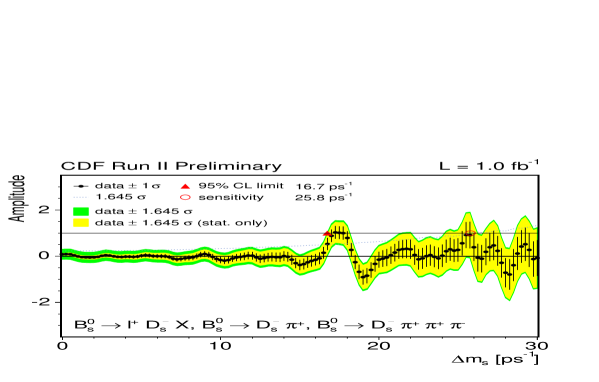
Figure 3.2: Amplitude of $B_{s}^{0}-\bar{B}_{s}^{0}$ oscillations as a function of the frequency $\Delta M_{s}$. These data proved that $B_{s}$ mesons oscillate, and measured their mass difference.

3.4.1 CP Asymmetries for $B$ decays

The small CP violation in mixing pointed out by (3.62) and (3.63) tells that $r$ is then a pure phase to an excellent approximation ($r\simeq e^{-i\phi_{\scriptscriptstyle M}}$, see (3.53)). The time dependent CP asymmetry for $B_{d,s}$ decays into CP eigenstates adopts now a quite simple form

$$\mathcal{A}_{\rm CP}(t)=\frac{\mathcal{A}_{\rm CP}^{dir}\cos{(\Delta Mt)}+\mathcal{A}_{\rm CP}^{mix}\sin{(\Delta Mt)}}{\cosh{(\Delta\Gamma t/2)}-\mathcal{A}_{\Delta\Gamma}\sinh{(\Delta\Gamma t/2)}}$$ (3.67)

which defines two quantities, the direct and mixing induced CP asymmetries, of capital importance in this thesis:

$$\mathcal{A}_{\rm CP}^{dir}\!\! \equiv \!\!\frac{1-|\lambda_{f}|^{2}}{1+|\lambda_{f}|^{2}}$$ (3.68)

$$\mathcal{A}_{\rm CP}^{mix}\!\! \equiv \!\!-\,\frac{2{\rm Im}\lambda_{f}}{1+|\lambda_{f}|^{2}}$$ (3.69)

and also

$$\mathcal{A}_{\Delta\Gamma}\equiv-\,\frac{2{\rm Re}\lambda_{f}}{1+|\lambda_{f}|^{2}}$$ (3.70)

These three quantities are not independent, but they are related through

$$|\mathcal{A}_{\rm CP}^{dir}|^{2}+|\mathcal{A}_{\rm CP}^{mix}|^{2}+|\mathcal{A}_{\Delta\Gamma}|^{2}=1$$ (3.71)

Let us take a look at the denominator in (3.67). When measuring the direct and mixing induced CP asymmetries, the oscillation period is the relevant time, $\tau_{\rm osc}\sim\Delta M^{-1}$. During an oscillation period the denominator in (3.67) is

$$\cosh{(\Delta\Gamma\,\tau_{\rm osc}/2)}-\mathcal{A}_{\Delta\Gamma}\sinh{(\Delta\Gamma\,\tau_{\rm osc}/2)}\sim 1+\mathcal{O}{\textstyle\left(\frac{\Delta\Gamma}{\Delta M}\right)}$$ (3.72)

And $\Delta\Gamma/\Delta M$ is very small for both $B_{d,s}$ systems. The time dependent CP asymmetry for $B$ decays into final CP eigenstates can then be written in the following form

$$\mathcal{A}_{\rm CP}(t)=\mathcal{A}_{\rm CP}^{dir}\cos{(\Delta Mt)}+\mathcal{A}_{\rm CP}^{mix}\sin{(\Delta Mt)}$$ (3.73)

In the case in which the relevant time is the lifetime, this is also basically true for $B_{d}$ mesons, due to eq. (3.64). However, the possibility of a large width difference for the $B_{s}$ system (e.g. (3.65)), might make possible the measurement of the asymmetries $\mathcal{A}_{\Delta\Gamma}$. This can be important for phenomenology, an example of which will be given in Chapter 6.

3.4.2 The $B_{d,s}-\bar{B}_{d,s}$ mixing angles and the $\Delta M_{d,s}$ mass differences

The experimental facts that $\Delta M_{d,s}\!\gg\!\Delta\Gamma_{d,s}$ and $|r|_{d,s}\simeq 1$, have implications on the value of $\Gamma_{12}^{d,s}/M_{12}^{d,s}$. In fact, from eqs. (3.20) and (3.21) one can solve for the real and imaginary parts of $\Gamma_{12}^{d,s}/M_{12}^{d,s}$ in terms of $|r|_{d,s}^{4}$ and $\Delta\Gamma_{d,s}/\Delta M_{d,s}$. In the limit $|r|_{d,s}\to 1$ and $\Delta\Gamma_{d,s}/\Delta M_{d,s}\to 0$, there is a trivial solution, $|\Gamma_{12}^{d,s}/M_{12}^{d,s}|\to 0$. However, this is not the only solution. The set of two nonlinear equations always gives two solutions. The first is the one close to zero, and the second is the one that makes $|\Gamma_{12}^{d,s}/M_{12}^{d,s}|$ a huge number, which for real data is of order $\sim 10^{3}$. This second solution is not realistic; for example in the SM, $\ |\Gamma_{12}/M_{12}|\sim m_{b}^{2}/m_{t}^{2}\sim 10^{-3}$. Therefore, data implies that

$$\left|\frac{\Gamma_{12}^{d,s}}{M_{12}^{d,s}}\right|\ll 1$$ (3.74)

When this result is plugged in eqs. (3.20) and (3.21), one gets

$$B\simeq|M_{12}|\ ,\quad r\simeq\sqrt{\frac{M_{12}^{*}}{M_{12}}}\ ,$$ (3.75)

such that

$$\Delta M_{d,s}\!\! \simeq 2|M_{12}^{d,s}|$$ (3.76)

$$\phi_{d,s} \simeq \arg{(M_{12}^{d,s})}$$ (3.77)

This means that in order to compute the mixing angles and the mass differences, it is enough to compute the mixing parameters $M_{12}^{d,s}$. Moreover, the expression (3.77) is sometimes taken as the definition of the mixing angle. One should keep in mind, however, that the mixing angle, as defined in this chapter, is not a physical quantity because it is sensitive to unphysical phase redefinitions. Therefore, it is important to work with a consistent convention for the weak phases everywhere; then the fact of assigning a numerical value to the mixing angle becomes sensible.

In some particular cases, ona can extract the mixing angle in a very clean way from a mixing induced CP asymmetry. Consider, for example, a decay into a CP eigenstate which is dominated by a single amplitude, which means that the dominant parts of the amplitude have all the same weak phase. Then, working in a convention in which the global weak phase is zero, one has

$$\lambda_{f}=e^{-i\phi_{\scriptscriptstyle M}}\frac{\bar{A}_{f}}{A_{f}}=\eta_{f}e^{-i\phi_{\scriptscriptstyle M}}\frac{\bar{A}_{\bar{f}}}{A_{f}}=\eta_{f}e^{-i\phi_{\scriptscriptstyle M}}\ ,$$ (3.78)

and hence $\ \mathcal{A}_{\rm CP}^{mix}=-{\rm Im}\lambda_{f}=\eta_{f}\sin{\phi_{\scriptscriptstyle M}}$. The prominent example is the case of $B_{d}\to J/\psi K_{s}$ [88]. Since this decay is dominated by a single amplitude, then $\bar{A}_{\overline{J/\psi K_{s}}}/A_{J/\psi K_{s}}\simeq\eta_{J/\psi K_{s}}=-1$, and therefore,

$$-\mathcal{A}_{\rm CP}^{mix}(B_{d}\to J/\psi K_{s})\simeq\sin{\phi_{d}}\ .$$ (3.79)

The neglected amplitude is both CKM and $\alpha_{s}(m_{b})$ suppressed with respect to the dominant amplitude, so the corrections to this equation are below the percent (or even the per mil) level [89, 90, 91].

3.5 CP Violation in the Standard Model

In this section we present the SM mechanism for CP violation; a simple and beautiful explanation formulated by M. Kobayashi and T. Maskawa in 1972 [73], only 5 years after the experimental discovery of CP violation. This formulation required also the existence of a third family of quarks (which had not yet been discovered), so together with the positive evidence of CP violation, this was a genuine prediction of the existence of the bottom and the top quarks.

Apart from the strong-CP issue –which we will not address here, and in any instance is a negligible effect–, the CP violation in the SM comes from the electroweak sector, and in particular from the Yukawa couplings. These couplings are described by the Glashow-Weinberg-Salam theory of EW interactions [92, 93, 94].

The GWS theory is a gauge theory based on the $SU(2)_{L}\otimes U(1)_{Y}$ group. The ‘L’ in $SU(2)_{L}$ indicates that the representations of the fermion fields depend on the chirality: Left-handed fermions are doublets and right-handed fermions are singlets. (This is how P violation is introduced in the SM.) Then, the kinetic terms in the lagrangian for the gauge and fermion fields are

$$\mathcal{L}_{K,F} = \bar{\psi}_{k_{L}}\,(i\partial/+gA/^{a}T^{a}+g^{\prime}B/\ Y_{k_{L}})\,\psi_{k_{L}}+\bar{\psi}_{k_{R}}\,(i\partial/+g^{\prime}B/\ Y_{k_{R}})\,\psi_{k_{R}}$$ (3.80)

$$\mathcal{L}_{K,G} = -\frac{1}{4}(F_{A}^{a,\,\mu\nu})^{2}-\frac{1}{4}(F_{B}^{\mu\nu})^{2}$$ (3.81)

where $A_{\mu}$, $B_{\mu}$ are the gauge fields, $T^{a}$ are the generators of $SU(2)$ in the fundamental representation, and a sum is understood over the left-handed and right-handed field species $k_{L,R}$. $F_{\mu\nu}$ are the usual field-strength tensors and $Y_{k}$ are the hypercharges of the fermion fields. Both kinetic terms are invariant under the full gauge group.

At this point a phenomenological problem arise. First, the chiral character of the gauge group spoils the gauge invariance of the fermion mass terms, so unbroken gauge symmetry forbids massive fermions in this theory. Second, gauge invariance forbids also mass terms for gauge bosons. The problem is that the observed fermions and gauge bosons that we want to describe are actually massive. The solution within the GWS theory is to postulate that the gauge symmetry is spontaneously broken.

The minimal realization of the spontaneous symmetry breaking (SSB) in the GWS theory is achieved by means of a single scalar $SU(2)$ doublet. This scalar field $\phi$, is assumed to acquire a vacuum expectation value $\langle\phi\rangle=v$, breaking spontaneously three independent linear combinations of generators and leaving unbroken the fourth combination. The unbroken combination of generators gives rise to the corresponding combination of the gauge fields that constitute the physical (massless) photon. The three broken combinations give rise to the appearance of three goldstone bosons, according to the Nambu-Goldstone theorem. These three degrees of freedom become, in an appropriate gauge, longitudinal polarization modes for the other three independent combinations of gauge bosons, which then acquire a mass. These three combinations can be chosen such that they have diagonal couplings with the photon (a definite electric charge). These are the physical $W^{\pm}$ and $Z$ bosons. The fourth remaining degree of freedom from the original complex scalar doublet $\phi$ is a physical real scalar field $h$, the higgs boson. In this way, the kinetic term for the scalar field $\phi$ can be written as

$$\mathcal{L}_{K,S}=(D^{\mu}\phi)^{\dagger}(D_{\mu}\phi)=\frac{1}{2}(\partial_{\mu}h)^{2}+\left[m_{W}^{2}W_{\mu}^{+}W^{-\,\mu}+\frac{1}{2}m_{Z}^{2}Z_{\mu}Z^{\mu}\right]\left(1+\frac{h}{v}\right)^{2}\ ,$$ (3.82)

with $\,m_{W}\equiv vg/2\,$ and $\,m_{Z}\equiv v\sqrt{g^{2}+g^{\prime 2}}/2\,$. This mechanism predicts a very definite relation between the masses of the $W$ and $Z$ bosons that was verified precisely at LEP. This solves the issue of the massive gauge bosons.

The kinetic term for the fermions (3.80) can then be expanded in terms of the physical gauge fields, and the charged and neutral weak currents identified. The electromagnetic currents then relate directly hypercharges and electric charges, and the hypercharge assignation can be made. The rest of the scalar lagrangian consists of an “opposite sign” $\phi$ mass term, $\mu\phi^{\dagger}\phi$, and an interaction term, $\lambda\phi^{4}$. In terms of physical fields these terms lead to interactions among gauge and higgs bossons, and to a higgs boson mass term. The parameters $\mu$ and $\lambda$ combine into $v$ and $m_{H}$, the higgs mass.

The issue of the massive fermions is still unsolved, and CP violation has not appeared yet in the theory. Here is where the things get interesting. For our purpose we focus on the quark fields $Q^{i}_{L}=(U^{i}_{L},D^{i}_{L})\$, $U^{i}_{R}$ and $D^{i}_{R}$. Having introduced the scalar doublet, gauge invariance allows (and hence requires) the following couplings between the fermions and the scalar,

$$\mathcal{L}_{Y} = -\lambda_{d}^{ij}\,\overline{Q^{i}_{L}}\cdot\phi\ D_{R}^{j}-\lambda_{u}^{ij}\,\epsilon^{ab}\,\overline{Q_{L}^{i}}_{a}\cdot\phi_{b}^{\dagger}\ U_{R}^{j}+{\rm h.c}$$ (3.83)

$$= -\frac{1}{\sqrt{2}}\lambda_{d}^{ij}\,\bar{D}_{L}^{i}D_{R}^{j}\,(v+h)-\frac{1}{\sqrt{2}}\lambda_{u}^{ij}\,\bar{U}_{L}^{i}U_{R}^{j}\,(v+h)+{\rm h.c}$$

where $a$, $b$ are $SU(2)$ indices. The parameters $\lambda^{ij}$ are arbitrary complex matrices in flavor space. This piece of the SM lagrangian provides masses for the quarks, quark-higgs interactions, and flavor mixing. Also, because the couplings can be complex, introduces the possibility of CP violation.

Now, to identify the masses, we must rotate the quark fields to get a diagonal mass matrix. The squared matrices $\lambda_{u}\!\cdot\!\lambda_{u}^{\dagger}$ and $\lambda_{u}^{\dagger}\!\cdot\!\lambda_{u}$ are hermitian, so they are diagonalizable with real and positive eigenvalues: $\lambda_{u}\!\cdot\!\lambda_{u}^{\dagger}=V_{u}D_{u}^{2}V_{u}^{\dagger}$, $\lambda_{u}^{\dagger}\!\cdot\!\lambda_{u}=W_{u}D_{u}^{2}W_{u}^{\dagger}$, with $D_{u}$ diagonal. The same is valid for $\lambda_{d}$. So $\lambda_{u}=V_{u}D_{u}W_{u}^{\dagger}$ and $\lambda_{d}=V_{d}D_{d}W_{d}^{\dagger}$. Then we rotate the fields such that

$$U_{L}^{i}=V_{u}^{ij}u_{L}^{j} U_{R}^{i}=W_{u}^{ij}u_{R}^{j}$$ ,

$$D_{L}^{i}=V_{d}^{ij}d_{L}^{j} D_{R}^{i}=W_{d}^{ij}d_{R}^{j}$$ , (3.84)

In terms of the rotated fields $u_{L,R}$ and $d_{L,R}$, the Yukawa lagrangian (3.83) becomes

$$\mathcal{L}_{Y}=-m_{d}^{i}\bar{d}_{L}^{i}d_{R}^{i}\left(1+\frac{h}{v}\right)-m_{u}^{i}\bar{u}_{L}^{i}u_{R}^{i}\left(1+\frac{h}{v}\right)$$ (3.85)

where $\ m_{q}^{i}\equiv vD_{q}^{ii}/\sqrt{2}\$ are the masses of the quarks.

This redefinition of the fields will only modify the fermionic part of the lagrangian $\mathcal{L}_{K,F}$, that is, the fermionic currents. In fact, it only modifies the charged currents, because the neutral currents are changed by things like $V^{\dagger}V=1$. The charged currents become

$$J_{W}^{+\,\mu}=\frac{1}{\sqrt{2}}\bar{U}_{L}^{i}\gamma^{\mu}D_{L}^{i}=\frac{1}{\sqrt{2}}\bar{u}_{L}^{i}\gamma^{\mu}V_{\scriptscriptstyle\rm CKM}^{ij}d_{L}^{j}$$ (3.86)

which defines the CKM matrix, $V_{\scriptscriptstyle\rm CKM}^{ij}\equiv(V_{u}^{\dagger}V_{d})^{ij}$. We see that in this mass eigenbasis for the quark fields, neutral currents are still diagonal, but the CKM matrix generates flavor-changing charged currents.

The CKM matrix can in principle be any square complex matrix in flavor space, since there is absolutely no constraint on the values of the Yukawa couplings $\lambda^{ij}$. The only constraint is unitarity, since $V_{\scriptscriptstyle\rm CKM}V_{\scriptscriptstyle\rm CKM}^{\dagger}=(V_{u}^{\dagger}V_{d})(V_{d}^{\dagger}V_{u})=1$. We are ready now to see how CP violation arises in this picture.

Consider first the case of 2 fermion families. The most general $2\times 2$ unitary matrix can be parameterized by one angle and three phases,

$$V_{\scriptscriptstyle\rm CKM}=\left(\begin{array}[]{cc}\cos{\theta_{\scriptscriptstyle C}}e^{i\alpha}&\sin{\theta_{\scriptscriptstyle C}}e^{i\beta}\\ -\sin{\theta_{\scriptscriptstyle C}}e^{i(\alpha+\gamma)}&\cos{\theta_{\scriptscriptstyle C}}e^{i(\beta+\gamma)}\\ \end{array}\right)$$ (3.87)

However, we may rephase the three of the four quark fields to remove the three phases. This means that for 2 fermion families, the CKM matrix can always be chosen to be real,

$$V_{\scriptscriptstyle\rm CKM}=\left(\begin{array}[]{cc}\cos{\theta_{\scriptscriptstyle C}}&\sin{\theta_{\scriptscriptstyle C}}\\ -\sin{\theta_{\scriptscriptstyle C}}&\cos{\theta_{\scriptscriptstyle C}}\\ \end{array}\right)$$ (3.88)

This is the Cabibbo matrix [95], and $\theta_{\scriptscriptstyle C}$ is the Cabibbo angle. The conclusion is that with only 2 fermion families, the SM cannot account for CP violation. This was the argument that led to the prediction of the third family of quarks, once CP violation was observed. For three generations of quarks, field rephasing cannot eliminate all the complex phases in the $3\times 3$ CKM matrix, but one complex fase is left. Therefore, the SM with 3 families predicts CP violation provided this phase is not zero. Another conclusion is that CP can only be violated in processes that involve the three families simultaneously, so in the SM, CP violation is generally a loop effect.

For numerical analyses, the most convenient parametrization of the CKM matrix is the standard parametrization [96]. However, a parametrization that makes its structure more clear is the Wolfenstein parametrization [97],

$$V_{\scriptscriptstyle\rm CKM}=\left(\begin{array}[]{ccc}V_{ud}&V_{us}&V_{ub}\\ V_{cd}&V_{cs}&V_{cb}\\ V_{td}&V_{ts}&V_{tb}\end{array}\right)=\left(\begin{array}[]{ccc}1-\frac{1}{2}\lambda^{2}&\lambda&A\lambda^{3}(\rho-i\eta)\\ -\lambda&1-\frac{1}{2}\lambda^{2}&A\lambda^{2}\\ A\lambda^{3}(1-\rho-i\eta)&-A\lambda^{2}&1\end{array}\right)+\mathcal{O}(\lambda^{4})$$ (3.89)

where $\lambda\equiv\sin{\theta_{\scriptscriptstyle C}}\simeq 0.22$ is treated as an expansion parameter. In this parametrization, the complex CP violating phase is

$$\gamma\equiv\arg\left(-\frac{V_{ud}V_{ub}^{*}}{V_{cd}V_{cb}^{*}}\right)=-\arg{(V_{ub})}+\mathcal{O}(\lambda^{4})=\arg{(\rho+i\eta)}+\mathcal{O}(\lambda^{4})\ ,$$ (3.90)

which up to order $\lambda^{4}$ is localized in $V_{ub}=|V_{ub}|e^{-i\gamma}$ and $V_{td}=|V_{td}|e^{-i\beta}$, and the rest of the entries are real. Here, $\beta$ is

$$\beta\equiv-\arg\left(-\frac{V_{td}V_{tb}^{*}}{V_{cd}V_{cb}^{*}}\right)=-\arg{(V_{td})}+\mathcal{O}(\lambda^{4})=\arg{(1-\rho+i\eta)}+\mathcal{O}(\lambda^{4})\ ,$$ (3.91)

and it is zero whenever $\gamma$ is zero. Therefore, in the SM, CP is violated if and only if $\gamma\neq 0$. Experimentally it is found that $\gamma\sim 60^{\circ}-70^{\circ}$. A convenient graphical picture is provided by the Unitarity Triangle, which arises from the unitarity of the CKM matrix, in particular from the unitarity relation $V_{ud}V_{ub}^{*}+V_{cd}V_{cb}^{*}+V_{td}V_{tb}^{*}=0$ (see Fig.3.3). CP violation can then be quantified by the area of this triangle. SM fits provide already a very consistent and constrained Unitarity Triangle, as we saw already in Fig.2.

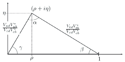
Figure 3.3: The unitarity triangle, and the definitions of the angles.

Let’s now take a look at the mixing angles in the SM for $B_{d}$ and $B_{s}$ mesons. We saw in the previous section that for $B_{q}$ mesons the given definition for the mixing angle is practically equivalent to $\phi_{\scriptscriptstyle M}=\arg{(M_{12})}$. We also saw in Section 3.1.1 that $M_{12}$ contains contributions from $H_{W}^{\scriptscriptstyle\Delta F=2}$ and also from transitions with intermediate on-shell states, at second order in $H_{W}^{\scriptscriptstyle\Delta F=1}$ (c.f. eq. 3.16). The contribution from intermediate on-shell states is mainly non-perturbative. It is an important contribution, for example, in kaon mixing. Fortunately, in the Standard Model the mixing of $B_{q}$ mesons is dominated by the perturbative $\Delta F=2$ box diagrams with a top quark in the loop (see Fig. 3.4).

\psfrag{b}{$b$}\psfrag{bb}{$\bar{b}$}\psfrag{q}{$q$}\psfrag{qb}{$\bar{q}$}\psfrag{t}{$t$}\psfrag{B}{$B_{q}$}\psfrag{Bb}{$\bar{B}_{q}$}\psfrag{Vb}{$V_{tb}^{*}$}\psfrag{Vq}{$V_{tq}$}\includegraphics[height=99.58464pt,width=369.88582pt]{SMMixingBoxes.eps}

Figure 3.4: Dominant SM contributions to the $B_{q}$-$\bar{B}_{q}$ mixing parameter $M_{12}^{q*}$. The CKM structure has been made explicit.

The CKM structure of these contributions is very simple. Both contributions are proportional to the product $(V_{tq}V_{tb}^{*})^{2}$: $M_{12}^{d*}\propto(V_{td}V_{tb}^{*})^{2}$ and $M_{12}^{s*}\propto(V_{ts}V_{tb}^{*})^{2}$. So it’s easy to see that the $B_{d}$-$\bar{B}_{d}$ mixing angle in the SM is given by

$$\phi_{d}^{\scriptscriptstyle SM}=2\beta+\mathcal{O}(\lambda^{4})\ .$$ (3.92)

The mixing angle $\phi_{s}^{\scriptscriptstyle SM}$ is zero is at this level of approximation, which means that enters in terms which are suppressed by at least $\lambda^{4}$. However, the phase itself is $\mathcal{O}(\lambda^{2})$. The angle $\beta_{s}$ is defined as

$$\beta_{s}\equiv-\arg{\left(-\frac{V_{ts}V_{tb}^{*}}{V_{cs}V_{cb}^{*}}\right)}\ .$$ (3.93)

Up to $\mathcal{O}(\lambda^{6})$, only $V_{ts}$ acquires a phase, so $V_{ts}=-|V_{ts}|e^{-i\beta_{s}}$. In fact $\beta_{s}\simeq-\lambda^{2}\eta$. Then, the $B_{s}$-$\bar{B}_{s}$ mixing angle in the SM is given by

$$\phi_{s}^{\scriptscriptstyle SM}=2\beta_{s}+\mathcal{O}(\lambda^{6})\ .$$ (3.94)

This is the way in which the mixing angles are related to the angles of the unitarity triangles in the Standard Model.

Appendix: CP-averaged branching ratio for 2-Body decays

The differential decay rate $d\Gamma$ for the decay of a particle $P$ in the center of mass (CM) frame into a final state $f$ is (see, for example, [98])

$$d\Gamma(P\to f)=\frac{1}{2m_{\scriptscriptstyle P}}\Big{(}\prod_{i}\frac{d^{3}p_{i}}{(2\pi)^{3}}\frac{1}{2E_{i}}\Big{)}\left|A(P\to f)\right|^{2}(2\pi)^{4}\delta(p_{\scriptscriptstyle P}-p_{f})$$ (3.95)

where $i$ runs over the set of particles in the final state with 4-momenta $p_{i}$ in the CM frame. $A(P\to f)$ is the amplitude of the process, and $m_{\scriptscriptstyle P}$ is the mass of the initial particle $P$ (the initial energy in the CM). For the case of 2 particles in the final state, the 4-momenta of the final particles are

$$p_{1}=(m_{\scriptscriptstyle P}/2+\Delta\,,k\hat{u})$$

$$p_{2}=(m_{\scriptscriptstyle P}/2-\Delta\,,-k\hat{u})$$ (3.96)

as described in Fig. 3.5.

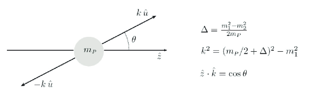
Figure 3.5: Kinematic description in the CM frame of the decay of a particle $P$ into two final particles. Conservation of 4-momenta imposed by the delta function in (3.95) implies the final state given by (3.96), with $\Delta$ and $k\hat{u}$ given in this figure. The axis $\hat{z}$ is chosen arbitrarily.

We can use the 4-delta function to integrate over the $\vec{p}_{2}$ 3-momenta and the modulus $|\vec{p}_{1}|$ in (3.95). This leads to the following general formula:

$$\left(\frac{d\Gamma}{d\Omega}\right)_{\!\rm CM}\!=\frac{k}{32\pi^{2}m_{\scriptscriptstyle P}^{2}}|A(P\to f)|^{2}$$ (3.97)

If the initial particle $P$ has spin 0, the process is spherically symmetric in the CM frame and the amplitude $A(P\to f)$ cannot have an angular dependence. In such a case the amplitude factorizes and the integrated decay rate can be written as

$$\Gamma(P\to f)=f_{\scriptscriptstyle\textrm{PS}}\,|A(P\to f)|^{2}$$ (3.98)

where $f_{\scriptscriptstyle\textrm{PS}}$ is called the phase space factor. This is just the angular integral which depends only on kinematic variables:

$$f_{\scriptscriptstyle\textrm{PS}}=\frac{1}{\sigma_{s}}\frac{k}{8\pi m_{\scriptscriptstyle P}^{2}}$$ (3.99)

Here $\sigma_{s}$ is a symmetry factor, which is $\sigma_{s}=1$ if the two final particles are distinguishable and $\sigma_{s}=2$ if they are identical. The meaning of this factor is that the final state with $\theta$ and that with $\theta+\pi$ are indistinguishable, and must be counted only once.

In the case of 2 particles with the same mass in the final state, we have $m_{1}\!=\!m_{2}\!\equiv\!m_{f}$, $\Delta=0$, and $k^{2}=(m_{\scriptscriptstyle P}^{2}-4m_{f}^{2})/4$, and the phase space factor is given by

$$f_{\scriptscriptstyle\textrm{PS}}=\frac{1}{\sigma_{s}}\frac{1}{16\pi m_{\scriptscriptstyle P}^{2}}\sqrt{m_{\scriptscriptstyle P}^{2}-4m_{f}^{2}}$$ (3.100)

The branching ratio $BR(P\to f)$ is defined as the partial decay rate $\Gamma(P\to f)$ divided by the total decay rate $\Gamma(P\to{\rm all})$. This quantity is naturally normalized to one, since the sum of the decay rates of all the exclusive decay modes of $P$ must equal $\Gamma(P\to{\rm all})$. The total decay rate is the inverse of the lifetime $\tau_{\scriptscriptstyle\textrm{P}}$. In “untagged” neutral meson decays, there is no information of whether the decaying particle is a $P^{0}$ or a $\bar{P}^{0}$. In such a case the measured branching ratio is an average between the decays $P^{0}\to f$ and $\bar{P}^{0}\to f$,

$$\overline{BR}(P^{0}\to f)=\frac{\Gamma(P^{0}\to f)+\Gamma(\bar{P}^{0}\to f)}{2\,\Gamma(P^{0}\to{\rm all})}=\tau_{\scriptscriptstyle\textrm{P}}f_{\scriptscriptstyle\textrm{PS}}\,\langle|A_{f}|^{2}\rangle$$ (3.101)

where $\langle|A_{f}|^{2}\rangle\equiv(|A_{f}|^{2}+|\bar{A}_{f}|^{2})/2=(|A_{f}|^{2}+|\bar{A}_{\bar{f}}|^{2})/2$, the last equality being true for $f$ a CP eigenstate. When the final state is a CP eigenstate then this is called a CP-averaged branching ratio. In this thesis we will only deal with CP-averaged branching ratios, so we will call them just $BR$, without the bar $\overline{BR}$. Moreover, we define the $g_{\scriptscriptstyle\textrm{PS}}$ factor as

$$g_{\scriptscriptstyle\textrm{PS}}\equiv\tau_{\scriptscriptstyle\textrm{P}}f_{\scriptscriptstyle\textrm{PS}}$$ (3.102)

Some numerical values for these factors, that will be used later, are

$$g_{\scriptscriptstyle\textrm{PS}}(B_{d}^{0}\to\pi^{+}\pi^{-})\ =\ 8.8\times 10^{9}\,{\rm GeV}^{-2}$$

$$g_{\scriptscriptstyle\textrm{PS}}(B_{d}^{0}\to K^{\scriptscriptstyle 0}\bar{K}^{\scriptscriptstyle 0})\ =\ 8.6\times 10^{9}\,{\rm GeV}^{-2}$$

$$g_{\scriptscriptstyle\textrm{PS}}(B_{s}^{0}\to K^{+}K^{-})\ =\ 8.1\times 10^{9}\,{\rm GeV}^{-2}$$

$$g_{\scriptscriptstyle\textrm{PS}}(B_{s}^{0}\to K^{\scriptscriptstyle 0}\bar{K}^{\scriptscriptstyle 0})\ =\ 8.1\times 10^{9}\,{\rm GeV}^{-2}$$ (3.103)

for input values of masses and lifetimes in [72] and using the conversion factor

$$1\,{\rm sec}=1.519\times 10^{24}\,{\rm GeV}^{-1}$$ (3.104)

For $B$ decays into two light mesons, the masses of the final mesons are sometimes neglected in front of $m_{B}$. If this is done, there are only two $g_{\scriptscriptstyle\textrm{PS}}$ factors: $g_{\scriptscriptstyle\textrm{PS}}(B_{d})=8.8\cdot 10^{9}\,{\rm GeV}^{-2}$ and $g_{\scriptscriptstyle\textrm{PS}}(B_{s})=8.2\cdot 10^{9}\,{\rm GeV}^{-2}$, which often simplifies the numerics.

Part II Applications

Chapter 4 Measuring New Physics in $B$ Decays

Up to now, the theoretical analyses of CP violation in B decays have been mostly focused on two complementary subjects. First, many different methods have been proposed for extracting in a clean way the CP violating angles $\alpha$, $\beta$ and $\gamma$, within the SM (see e.g. [72, 85]). We have now many ways of checking the compatibility of different measurements within the SM and detect the presence of NP. Second, many studies have been made of observables within specific scenarios of NP in the forward direction; that is: what values for these observables does this specific model predict? These second type of studies are important because they provide a direct bridge between new data and the reduction of the allowed regions in the NP parameter spaces. In an extreme situation, they may even rule out some models (see for example [99]).

However, the identification of the NP, once this is found, requires NP studies in the inverse direction; that is: given this non-standard experimental data, what is the NP that describes it? This “inverse problem” is rather complex because of two reasons. First, given a specific model, a signature in observable space is generally associated to many points in parameter space (“degeneracies”). In the most unfavorable situation this can be a huge continuously connected region, meaning that this signature in observable space will give absolutely no clue on the basic structure of the underlying theory (for a study of the inverse problem in supersymmetry see [100]). Second, the most important information that must be extracted from NP signals is related to general characteristics of the NP. Indeed, solving the inverse problem in supersymmetry is of no help if nature turns out not to be supersymmetric. But model independent analyses of NP are generally unapproachable because of the large number of parameters involved (see the discussion in Section 1.3), so at the end one has to come up with arguments that allow to reduce the number of model independent NP parameters.

A first step in this direction was taken in Ref. [101], where it was shown that an argument concerning new physics strong phases allows to reduce the number of NP parameters to a manageable level, and measure them. The knowledge of these model independent NP parameters allows then to identify partially the new physics, and to establish some of its generic features.

In this chapter we present an approach, within this framework, to measure the NP parameters that appear in $B_{s}\to K^{+}K^{-}$ amplitudes. This approach requires experimental information on branching ratios and CP asymmetries in $B_{d}\to\pi^{+}\pi^{-}$ and $B_{s}\to K^{+}K^{-}$, and is based on a SU(3) analysis of these modes and the (motivated) assumption that any NP contributing to $\bar{b}\to\bar{d}$ penguin amplitudes is negligible at the considered level of approximation.

4.1 Parametrization of the SM Amplitudes

The SM amplitude of a generic two body non-leptonic B decay ($B_{q}\to M_{1}M_{2}$) is commonly parameterized in terms of its CKM structure. We used this fact already in the discussion of strong and weak phases in Section 3.3, where it was justified by invoking the form of the SM effective Hamiltonian as written in Eq. (1.27). However, we have never proved here that the Wilson coefficients in Eq. (1.27) are CKM independent; in fact, strictly speaking, they are not.

In this chapter we abandon temporarily the effective Hamiltonian description of the amplitudes, in favor of a diagrammatic approach that makes this CKM issue more transparent.

We will restrict ourselves to a general situation in which the parametrization of Eq. (3.59) holds: decays which contain contributions from tree or penguin diagrams where the two up-type quarks produced in the decay (if any) are both either up or charm quarks. The leading contributions, which contain a single $W$ propagator, are then all proportional to either one of the CKM products $V_{uD}V^{*}_{ub}$, $V_{cD}V^{*}_{cb}\$ or $\ V_{tD}V^{*}_{tb}$, where $D$ is the down-type quark in the final state which is not $q$ (see Fig. 4.1).

(-419,37)[lb]$B_{q}$ (-342,13)[lb]$M_{\scriptscriptstyle 1}$ (-341,67)[lb]$M_{\scriptscriptstyle 2}$ (-400,47)[lb]$\bar{b}$ (-375,24)[lb]$q$ (-345,40)[lb]$\bar{U}$ (-356,54)[lb]$U^{\prime}$ (-357,79)[lb]$\bar{D}$ (-385,-5)[lb]$(a)$ (-309,37)[lb]$B_{q}$ (-233,13)[lb]$M_{\scriptscriptstyle 1}$ (-234,67)[lb]$M_{\scriptscriptstyle 2}$ (-290,47)[lb]$\bar{b}$ (-265,24)[lb]$q$ (-240,27)[lb]$\bar{D}$ (-240,50)[lb]$U^{\prime}$ (-250,75)[lb]$\bar{U}$ (-275,-5)[lb]$(b)$ (-200,37)[lb]$B_{q}$ (-124,13)[lb]$M_{\scriptscriptstyle 1}$ (-125,67)[lb]$M_{\scriptscriptstyle 2}$ (-180,47)[lb]$\bar{b}$ (-155,23)[lb]$q$ (-132,27)[lb]$\bar{Q}$ (-132,50)[lb]$Q$ (-142,75)[lb]$\bar{D}$ (-167,45)[lb]$\bar{u},\!\bar{c},\!\bar{t}$ (-165,-5)[lb]$(c)$ (-92,37)[lb]$B_{q}$ (-15,13)[lb]$M_{\scriptscriptstyle 1}$ (-14,67)[lb]$M_{\scriptscriptstyle 2}$ (-72,45)[lb]$\bar{b}$ (-45,24)[lb]$q$ (-15,40)[lb]$\bar{D}$ (-26,54)[lb]$Q$ (-27,79)[lb]$\bar{Q}$ (-56,63)[lb]$\bar{u},\!\bar{c},\!\bar{t}$ (-55,-5)[lb]$(d)$

Figure 4.1: Leading contributions to $B_{q}\to M_{1}M_{2}$ which do not involve the spectator quark ($\bar{b}\to\bar{D}q\bar{q}$). The quark labels stand for $q,Q=\{u,d,s,c\}$, $U,U^{\prime}=\{u,c\}\$ and $D=\{d,s\}$. The color allowed (a) and color suppressed (b) tree amplitudes are proportional to $V_{\scriptscriptstyle U^{\prime}\!\!D}V^{*}_{\scriptscriptstyle U\!b}$. The color suppressed and color allowed penguin amplitudes (c) and (d) are proportional to $V_{\scriptscriptstyle\ell\!D}V^{*}_{\scriptscriptstyle\ell\!b}$, where $\ell=\{u,c,t\}$ is the quark inside the loop. Note that not all of the diagrams contribute to a given decay.

Because in a given decay the CKM elements always enter by pairs, it is customary to define the following product of CKM elements, $\lambda_{\ell}^{\scriptscriptstyle(D)}\equiv V_{\scriptscriptstyle\ell\!D}^{*}V_{\scriptscriptstyle\ell\!b}$. Moreover, the unitarity of the CKM matrix implies the triangle relation

$$\lambda_{u}^{\scriptscriptstyle(D)}+\lambda_{c}^{\scriptscriptstyle(D)}+\lambda_{t}^{\scriptscriptstyle(D)}=0$$ (4.1)

which allows to eliminate the CKM factor $\lambda_{t}^{\scriptscriptstyle(D)}$ from the amplitude. The amplitude is then a sum of two terms, proportional to $\lambda_{u}^{\scriptscriptstyle(D)}$ and $\lambda_{c}^{\scriptscriptstyle(D)}$ respectively. We define the “tree” ($T_{\scriptscriptstyle\!M_{1}\!M_{2}}^{q}$) and the “penguin” ($P_{\scriptscriptstyle\!M_{1}\!M_{2}}^{q}$) amplitudes as the coefficients of the two terms with different CKM structures. Thus the amplitude can be written as

$$A(B_{q}\to M_{1}M_{2})=\lambda_{u}^{\scriptscriptstyle(D)*}\,T_{\scriptscriptstyle\!M_{1}\!M_{2}}^{q}+\lambda_{c}^{\scriptscriptstyle(D)*}P_{\scriptscriptstyle\!M_{1}\!M_{2}}^{q}$$ (4.2)

Besides the topologies shown in Fig. 4.1, there are also leading contributions which involve the spectator quark, mainly exchange, annihilation and penguin annihilation diagrams [102]. However, it has been argued that these can be neglected at leading order, since they imply the fairly unlikely situation in which the two quarks inside the B meson annihilate each other or interact weakly before the decay of the $b$ quark. This is called the spectator quark hypothesis, and as any other hypothesis it should be handled with care (for example, these contributions could be Cabibbo enhanced). Unlike the penguin annihilation topology, the exchange and annihilation contributions do not in general obey the CKM structure discussed above, and do not fit in the scheme. However, for charmless decays and decays into CP eigenstates they do, and they can be included in the description trivially. Since we will be focusing our discussion in two-body decays of neutral B mesons ($q=d,s$) into CP eigenstates, this issue will be of no concern.

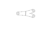
(-310,37)[lb]$B_{q}^{0}$ (-233,13)[lb]$M_{\scriptscriptstyle 1}$ (-233,67)[lb]$M_{\scriptscriptstyle 2}$ (-290,48)[lb]$\bar{b}$ (-290,28)[lb]$q$ (-250,17)[lb]$U^{\prime}$ (-241,27)[lb]$\bar{Q}$ (-240,50)[lb]$Q$ (-250,75)[lb]$\bar{U}$ (-275,-15)[lb]$(a)$ (-201,37)[lb]$B_{q}^{+}$ (-124,13)[lb]$M_{\scriptscriptstyle 1}$ (-124,67)[lb]$M_{\scriptscriptstyle 2}$ (-184,58)[lb]$\bar{b}$ (-184,21)[lb]$q$ (-132,25)[lb]$Q$ (-132,50)[lb]$\bar{Q}$ (-145,75)[lb]$U$ (-145,4)[lb]$\bar{D}$ (-170,-15)[lb]$(b)$ (-91,37)[lb]$B_{q}^{0}$ (-15,13)[lb]$M_{\scriptscriptstyle 1}$ (-15,67)[lb]$M_{\scriptscriptstyle 2}$ (-75,60)[lb]$\bar{b}$ (-75,19)[lb]$q$ (-23,25)[lb]$Q$ (-23,50)[lb]$\bar{Q}$ (-36,75)[lb]$Q^{\prime}$ (-36,3)[lb]$\bar{Q}^{\prime}$ (-60,27)[lb]$u,\!c,\!t$ (-55,-15)[lb]$(c)$

Figure 4.2: Exchange (a), Annihilation (b) and Penguin Annihilation (c) contributions. (a) and (c) only exist for $q=\{d,s\}$ and (b) only exists for $q=\{u,c\}$. The penguin annihilation contribution always fits in the structure (4.2). The exchange and annihilation topologies only have such CKM structure for $U=U^{\prime}$ and $q=U$ respectively. For final CP eigenstates this structure is automatically satisfied (there is no annihilation contribution in this case).

To be specific, the tree and penguin contributions, in terms of the diagrams in Fig. 4.1, are given by

$$T_{\scriptscriptstyle\!M_{1}\!M_{2}}^{q} = T_{u}+C_{u}+(P_{u}-P_{t})+(P^{C}_{u}-P^{C}_{t})$$

$$P_{\scriptscriptstyle\!M_{1}\!M_{2}}^{q} = T_{c}+C_{c}+(P_{c}-P_{t})+(P^{C}_{c}-P^{C}_{t})$$ (4.3)

where $\lambda_{U}^{\scriptscriptstyle(D)*}T_{U}$, $\lambda_{U}^{\scriptscriptstyle(D)*}C_{U}$, $\lambda_{\ell}^{\scriptscriptstyle(D)*}P_{\ell}$ and $\lambda_{\ell}^{\scriptscriptstyle(D)*}P^{C}_{\ell}$ are respectively the amplitudes (a), (b), (d) and (c) in Fig. 4.1.

The CKM products $\lambda_{U}^{\scriptscriptstyle(D)}$ have the following numerical values [72]:

$$\lambda_{u}^{(d)}=0.0038e^{i\gamma}=|\lambda_{u}^{(d)}|e^{-i\gamma}\qquad \lambda_{c}^{(d)}=-0.0094=-|\lambda_{c}^{(d)}|$$ (4.4)

$$\lambda_{u}^{(s)}=0.00088e^{i\gamma}=|\lambda_{u}^{(s)}|e^{-i\gamma}\qquad \lambda_{c}^{(s)}=0.04=|\lambda_{c}^{(s)}|$$

where $\gamma$ is the CKM weak phase. Note the negative sign of $\lambda_{c}^{(d)}$. We denote the relative (strong) phase between $T_{\scriptscriptstyle\!M_{1}\!M_{2}}^{q}$ and $P_{\scriptscriptstyle\!M_{1}\!M_{2}}^{q}$ by $\,\theta_{\scriptscriptstyle\!M_{1}\!M_{2}}^{q}$:

$$\theta_{\scriptscriptstyle\!M_{1}\!M_{2}}^{q}\equiv arg\left(\frac{P_{\scriptscriptstyle\!M_{1}\!M_{2}}^{q}}{T_{\scriptscriptstyle\!M_{1}\!M_{2}}^{q}}\right)$$ (4.5)

Now we can give a general useful parameterization of the amplitude in (4.2),

$$A(B_{q}\to M_{1}M_{2})=|\lambda_{u}^{\scriptscriptstyle(D)}||T|e^{i\delta_{T}}\left(e^{i\gamma}\pm\left|\frac{\lambda_{c}^{\scriptscriptstyle(D)}}{\lambda_{u}^{\scriptscriptstyle(D)}}\right|\left|\frac{P}{T}\right|e^{i\theta}\right)=|\lambda_{u}^{\scriptscriptstyle(D)}||T|e^{i\delta_{T}}\left(e^{i\gamma}\pm de^{i\theta}\right)$$ (4.6)

the plus (minus) sign being for $D=s$ ($D=d$). We have dropped the labels $q$ and $M_{1}M_{2}$ for simplicity, and it will be done so systematically whenever there is no ambiguity. We have also defined [65]

$$d=d_{\scriptscriptstyle\!M_{1}\!M_{2}}^{q}\equiv\left|\frac{\lambda_{c}^{\scriptscriptstyle(D)}}{\lambda_{u}^{\scriptscriptstyle(D)}}\right|\left|\frac{P_{\scriptscriptstyle\!M_{1}\!M_{2}}^{q}}{T_{\scriptscriptstyle\!M_{1}\!M_{2}}^{q}}\right|$$ (4.7)

and $\delta_{T}$ is the strong phase associated to $T_{\scriptscriptstyle\!M_{1}\!M_{2}}^{q}$. Note that when (4.6) is the full amplitude (that is, when there are no NP contributions), the phase $\delta_{T}$ is not physical and does not appear in the observables. The amplitude for the CP-conjugate process $\bar{B}_{q}\to\bar{M}_{1}\bar{M}_{2}$ shall be obtained from (4.6) by changing the sign of the weak phase $\gamma$.

4.2 Measuring the SM parameters

Assuming that no new contributions come into play, and that the full amplitude is described within SM as in (4.6), it is possible to measure the SM hadronic parameters $T_{\scriptscriptstyle\!M_{1}\!M_{2}}^{q}$, $P_{\scriptscriptstyle\!M_{1}\!M_{2}}^{q}$ and $\theta_{\scriptscriptstyle\!M_{1}\!M_{2}}^{q}$. There are three potential experimental measurements that can be carried out in neutral B decays that allow us to extract this information. These are the CP-averaged branching ratio (see the Appendix to Chapter 3), the direct CP asymmetry and the mixing induced CP asymmetry (see section 3.4). By virtue of the formulae (3.101), (3.68) and (3.69) one can relate these observables to the theoretical parameters in (4.6):

$$BR=g_{\scriptscriptstyle\textrm{PS}}|\lambda_{u}^{\scriptscriptstyle(D)}|^{2}|T|^{2}\left(1+d^{2}\pm 2d\cos{\gamma}\cos{\theta}\right)$$ (4.8)

$$\mathcal{A}_{\rm CP}^{dir}=\pm\frac{2d\sin{\gamma}\sin{\theta}}{1+d^{2}\pm 2d\cos{\gamma}\cos{\theta}}$$ (4.9)

$$\mathcal{A}_{\rm CP}^{mix}=\frac{\sin{(2\gamma+\phi_{\scriptscriptstyle M})}\pm 2d\sin{(\gamma+\phi_{\scriptscriptstyle M})}\cos{\theta}+d^{2}\sin{\phi_{\scriptscriptstyle M}}}{1+d^{2}\pm 2d\cos{\gamma}\cos{\theta}}$$ (4.10)

where, again, the plus and minus signs correspond to $D=s$ and $D=d$, respectively.

The hadronic parameters $|T|$, $d$ and $\theta$ are specific of each particular decay. The CKM angle $\gamma$ and the mixing angle $\phi_{\scriptscriptstyle M}$ are, on the contrary, universal theoretical parameters, and can be obtained from a multitude of different decays. Therefore, we are left with three hadronic parameters ($|T|$, $d$ and $\theta$) to be obtained from three experimental values ($BR$, $\mathcal{A}_{\rm CP}^{dir}$ and $\mathcal{A}_{\rm CP}^{mix}$) by means of equations (4.8)-(4.10).

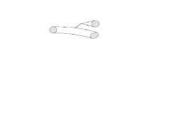
(-329,44)[lb]$B_{d}^{0}$ (-211,15)[lb]$\pi^{-}$ (-209,78)[lb]$\pi^{+}$ (-300,54)[lb]$\bar{b}$ (-265,29)[lb]$d$ (-230,95)[lb]$\bar{d}$ (-230,66)[lb]$u$ (-230,39)[lb]$\bar{u}$ (-275,-5)[lb]$(a)$ (-136,44)[lb]$B_{d}^{0}$ (-18,15)[lb]$\pi^{-}$ (-19,78)[lb]$\pi^{+}$ (-110,55)[lb]$\bar{b}$ (-70,27)[lb]$d$ (-30,33)[lb]$\bar{u}$ (-30,60)[lb]$u$ (-42,75)[lb]$\bar{d}$ (-75,-5)[lb]$(b)$ (-82,46)[lb]$\bar{u},\!\bar{c},\!\bar{t}$

Figure 4.3: Leading diagrams contributing to the decay $B_{d}^{0}\to\pi^{+}\pi^{-}$, (a) tree and (b) penguin contributions.

As a matter of illustration and for later usage, consider the decay $B_{d}^{0}\to\pi^{+}\pi^{-}$. At the quark level (see Fig. 4.3) it corresponds to a $\bar{b}\to\bar{d}$ transition ($D=d$), so we must choose the minus sign in (4.8)-(4.10). For the branching ratio and the CP asymmetries we take an average of the Babar and Belle data [103, 104, 105],

$$BR(B_{d}^{0}\rightarrow\pi^{+}\pi^{-})_{\rm exp} = (5.0\pm 0.4)\times 10^{-6}$$ (4.11)

$$\mathcal{A}_{\rm CP}^{dir}(B_{d}^{0}\rightarrow\pi^{+}\pi^{-})_{\rm exp} = -0.33\pm 0.11$$ (4.12)

$$\mathcal{A}_{\rm CP}^{mix}(B_{d}^{0}\rightarrow\pi^{+}\pi^{-})_{\rm exp} = 0.49\pm 0.12$$ (4.13)

Because $\mathcal{A}_{\rm CP}^{dir}$ and $\mathcal{A}_{\rm CP}^{mix}$ do not depend on the magnitude of the tree (c.f. (4.9), (4.10)), the calculation of the hadronic parameters can be divided in two steps. First we vary the asymmetries inside their experimental range to find the allowed region in the $d-\theta$ plane. This is illustrated in Fig. 4.4. Second, we vary the branching ratio in its range together with the allowed values of $d$ and $\theta$, to find the range for $|T|$ according to (4.8). The results are shown in Table 4.1.

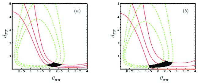
Figure 4.4: Allowed regions in the $d-\theta$ plane for $B_{d}^{0}\to\pi^{+}\pi^{-}$, (a) taking $\gamma=61^{\circ}$ and (b) varying $\gamma$ in the range $\gamma=(61^{+7}_{-5})^{\circ}$. The dashed lines show the central value and $\pm 1\sigma$ deviations for $\mathcal{A}_{\rm CP}^{dir}(B_{d}^{0}\to\pi^{+}\pi^{-})$, and the solid lines the same for $\mathcal{A}_{\rm CP}^{mix}(B_{d}^{0}\to\pi^{+}\pi^{-})$.

	$d_{\pi\pi}$	$\theta_{\pi\pi}$ (deg)	$\left|T_{\pi\pi}\right|(10^{-6}{\rm GeV})$	$\left|P_{\pi\pi}/T_{\pi\pi}\right|$
$\begin{array}[]{c}\gamma=61^{\circ}\\ \end{array}$	$(0.18,0.49)$	$(107,150)$	$(4.87,6.11)$	$(0.07,0.20)$
$\begin{array}[]{c}\gamma=(61^{+7}_{-5})^{\circ}\\ \end{array}$	$(0.14,0.61)$	$(88,158)$	$(4.60,6.45)$	$(0.06,0.25)$

Table 4.1: Allowed ranges for the hadronic parameters in the decay $B_{d}^{0}\to\pi^{+}\pi^{-}$, calculated from the experimental values for the branching ratio and the two CP asymmetries. The values are taken from an average of Babar and Belle data. The sensibility on the error of $\gamma$ is shown. The penguin-to-tree ratio is obtained from $d$ and (4.7).

Note that two different solutions in the $d-\theta$ plane are allowed by a single value of the pair $(\mathcal{A}_{\rm CP}^{dir},\mathcal{A}_{\rm CP}^{mix})$ (see the two separate regions in Figs. 4.4). This is due to the non-linearity of the equations (4.9) and (4.10). However, it should be clear that only one solution corresponds to a given pair $(T,P)$, so only one of the two regions in the $d-\theta$ can be physical. QCDF predicts a value for $d_{\pi\pi}$ around $0.3$ [27], so the second solution ($d_{\pi\pi}>3$) is likely to be the non-physical one and it’s ruled out. This is also confirmed independently by an analysis concerning the channel $B_{d}\to\pi^{\mp}K^{\pm}$ [106].

4.3 Parameterization of the New Physics Amplitudes

Besides the SM contributions, a given decay might also receive contributions from physics beyond the SM. Without a specific model for the NP, they cannot be calculated. However, it is possible to make a model independent parameterization of these contributions under certain general circumstances [101].

In the context of the low energy effective Hamiltonian, the new contributions will be of two types. First, there will be new contributions to the Wilson Coefficients of the SM operators. Second, new operators will appear which are not generated by the SM. To this end we write the effective Hamiltonian as a sum of the SM and NP contributions:

$$\mathcal{H}_{\rm eff}=\mathcal{H}_{\scriptscriptstyle\rm SM}+\mathcal{H}_{\scriptscriptstyle\rm NP}$$ (4.14)

Because the nature of the NP is unknown, $\mathcal{H}_{\scriptscriptstyle\rm NP}$ contains all possible operators compatible with a given process. As it will become clear below, we are mainly interested on the NP contributions to $\bar{b}\to\bar{s}q\bar{q}$ transitions. There are 20 dimension-six operators that contribute potentially to such decays, and the general NP effective Hamiltonian in (4.14) can be written as

$$\mathcal{H}_{\scriptscriptstyle\rm NP}^{q}={\displaystyle\sum_{\scriptscriptstyle A,B=L,R}\frac{G_{F}}{\sqrt{2}}} \Big{[}\,f^{\scriptscriptstyle AB}_{q,1}\,\bar{s}_{\alpha}\gamma_{A}b_{\beta}\,\bar{q}_{\beta}\gamma_{B}q_{\alpha}+f^{\scriptscriptstyle AB}_{q,2}\,\bar{s}\gamma_{A}b\,\bar{q}\gamma_{B}q$$ (4.15)

$$+g^{\scriptscriptstyle AB}_{q,1}\,\bar{s}_{\alpha}\gamma^{\mu}\gamma_{A}b_{\beta}\,\bar{q}_{\beta}\gamma_{\mu}\gamma_{B}q_{\alpha}+g^{\scriptscriptstyle AB}_{q,2}\,\bar{s}\gamma^{\mu}\gamma_{A}b\,\bar{q}\gamma^{\mu}\gamma_{B}q$$

$$+h^{\scriptscriptstyle AB}_{q,1}\,\bar{s}_{\alpha}\sigma^{\mu\nu}\gamma_{A}b_{\beta}\,\bar{q}_{\beta}\sigma_{\mu\nu}\gamma_{B}q_{\alpha}+h^{\scriptscriptstyle AB}_{q,2}\,\bar{s}\sigma^{\mu\nu}\gamma_{A}b\,\bar{q}\sigma_{\mu\nu}\gamma_{B}q\,\Big{]}$$

where $\gamma_{\scriptscriptstyle R,L}\equiv\frac{1}{2}(1\pm\gamma_{5})$. The coefficients in (4.15) will in general contain new (model dependent) weak phases and the matrix elements of these operators will introduce new (process dependent) strong phases. The strong phases, as mentioned in section 3.3, come mainly from rescattering. The important point is that the NP strong phases must come from rescattering of NP operators. Let’s discuss this in more detail.

In the SM, the strong phases may be large and must be taken into account because they arise from rescattering of tree operators, and although the process of rescattering is size-consuming (the rescattered penguin amplitudes are about 5-10% of the tree amplitudes), the tree amplitudes are big and the rescattered penguins can be as large as the SM penguin amplitudes. This situation holds even when there are no tree operators that contribute directly to the decay, since these can contribute through rescattering. In such cases, the rescattered penguin can be of the same order of the largest contributions.

The NP operators, however, are expected to give direct contributions not larger than the SM penguin contributions. This means that the rescattering from such NP operators will be at most 5-10% as big as the SM penguins, and at the level of other neglected diagrams. We can therefore argue that these small contributions can be neglected, and since these are the main sources of new strong phases, the strong phases can be approximately set to zero in the NP amplitude. Thus, without strong phases, the NP amplitude can be parameterized in terms of a single effective weak phase:

$$\langle f|\mathcal{H}_{\scriptscriptstyle\rm NP}^{q}|B\rangle\equiv\mathcal{A}^{q}e^{i\Phi_{q}}$$ (4.16)

Note that there is a potential loop-hole in this argument. We can be sure about the size of the largest NP contributions to the decay in consideration, and thus be confident in neglecting the strong phases coming from the rescattering of these diagrams. However, the possibility remains of the existence of NP diagrams which do not contribute directly but through rescattering to the given decay. If they were much larger than the SM penguins that do contribute, they could introduce sizeable strong phases in the NP amplitude. Other cases which get around this reasoning are when the NP is light, or if there is a significant enhancement of certain matrix elements.

4.4 Hints of New Physics in B decays

The question arises of whether we should expect sizeable contributions from physics beyond the SM, or if these, even if they exist, are too small to be observed at present. A second question would be what transitions are likely to be appreciably affected by NP. There are several indications that may help to answer these questions. For example, the CP asymmetry in $\bar{b}\to\bar{s}q{\bar{q}}$ modes ($q=u,d,s$) is found to differ from that in ${\bar{b}}\to{\bar{c}}c{\bar{s}}$ decays by 2.6$\sigma$ (they are expected to be approximately equal in the SM) [86, 107]. In addition, some $B\to\pi K$ measurements disagree with SM expectations [108, 109], although the so-called $B\to\pi K$ puzzle [110, 111, 112, 106, 113] has been reduced [114, 115, 116, 117]. One also sees a discrepancy with the SM in triple-product asymmetries in $B\to\phi K^{*}$ [118, 119, 120], and in the polarization measurements of $B\to\phi K^{*}$ [121, 122] and $B\to\rho K^{*}$ [72, 123, 124]. These discrepancies are (almost) all not yet statistically significant, being in the 1–2$\sigma$ range. However, if these hints are taken together, the statistical significance increases. Furthermore, they are intriguing since they all point to New Physics in $\bar{b}\to\bar{s}$ transitions. For this reason it is interesting to consider the effect of NP on $B$ decays dominated by the quark-level $\bar{b}\to\bar{s}$ transition, and assume that no NP affects $\bar{b}\to\bar{d}$ transitions.

4.5 Measuring the New Physics parameters through Flavor Symmetries

For the sake of clarity we begin this section summarizing the basic ideas discussed so far.

The amplitudes for B decays that at the quark level are governed by the transition $\bar{b}\to\bar{D}q\bar{q}$, can be written as

$$A(\bar{b}\to\bar{d}q\bar{q})=|\lambda_{u}^{\scriptscriptstyle(d)}||T|\left(e^{i\gamma}-de^{i\theta}\right)$$ (4.17)

$$A(\bar{b}\to\bar{s}q\bar{q})=|\lambda_{u}^{\scriptscriptstyle(s)}||T^{\prime}|e^{i\delta_{T}}\left(e^{i\gamma}+d^{\prime}e^{i\theta^{\prime}}\right)+\mathcal{A}^{q}e^{i\Phi_{q}}$$ (4.18)

These parameterizations rely on several conditions:

• SM diagrams which do not obey the CKM structure in (4.2) can be neglected with respect to the penguin amplitudes.

• Potential NP contributions to $\bar{b}\to\bar{d}$ decays can be neglected with respect to the SM penguin amplitudes.

• There are no NP operators large enough to produce a sizeable contribution to the $\bar{b}\to\bar{s}$ decay through rescattering.

In section 4.2 we showed how to measure the SM hadronic parameters in (4.6) from measurements on the branching ratio and the CP-asymmetries. The method was applied to obtain the hadronic parameters of the decay $B_{d}^{0}\to\pi^{+}\pi^{-}$, that according to the previous conditions it is described entirely within SM as in (4.17). The same could be done, in principle, with a $\bar{b}\to\bar{s}$ decay. Taking the amplitude in (4.18), the branching ratio and the asymmetries can be expressed in terms of the SM hadronic parameters and the NP parameters. The expressions are much more complicated in this case:

$$BR=BR^{\scriptscriptstyle\rm SM}\cdot(1+\mathcal{B}^{\scriptscriptstyle\rm NP})$$ (4.19)

$$\mathcal{A}_{\rm CP}^{dir}=\frac{A_{dir}^{\scriptscriptstyle\rm SM}+\mathcal{D}^{\scriptscriptstyle\rm NP}}{1+\mathcal{B}^{\scriptscriptstyle\rm NP}}$$ (4.20)

$$\mathcal{A}_{\rm CP}^{mix}=\frac{A_{mix}^{\scriptscriptstyle\rm SM}\cdot\cos{\delta\phi_{s}^{\scriptscriptstyle\rm NP}}+\mathcal{M}^{\scriptscriptstyle\rm NP}}{1+\mathcal{B}^{\scriptscriptstyle\rm NP}}$$ (4.21)

where the SM functions $BR^{\scriptscriptstyle\rm SM}$, $A_{dir}^{\scriptscriptstyle\rm SM}$ and $A_{mix}^{\scriptscriptstyle\rm SM}$ are those in (4.8)-(4.10) taking the plus sign and $D=s$, and the NP functions are given by

$$\mathcal{B}^{\scriptscriptstyle\rm NP}=\frac{1}{\Delta}\big{\{}z^{2}+2z[\cos{(\Phi_{q}-\gamma)}\cos{\delta_{T}}+d\cos{\Phi_{q}}\cos{(\theta+\delta_{T})}]\big{\}}$$ (4.22)

$$\mathcal{D}^{\scriptscriptstyle\rm NP}=\frac{1}{\Delta}\big{\{}2z[\sin{(\Phi_{q}-\gamma)}\sin{\delta_{T}}+d\sin{\Phi_{q}}\sin{(\theta+\delta_{T})}]\big{\}}$$ (4.23)

$$\mathcal{M}^{\scriptscriptstyle\rm NP}= \frac{1}{\Delta}\big{\{}z^{2}\sin{(2\Phi_{q}+\phi_{s})}+2z[\sin{(\Phi_{q}+\phi_{s}+\gamma)}\cos{\delta_{T}}+d\cos{(\theta+\delta_{T})}\sin{(\Phi_{q}+\phi_{s})}]$$ (4.24)

$$+\,[\cos{(2\gamma+\phi_{s}^{\scriptscriptstyle\rm SM})}+2d\cos{(\theta)}\cos{(\gamma+\phi_{s}^{\scriptscriptstyle\rm SM})}+d^{2}\cos{\phi_{s}^{\scriptscriptstyle\rm SM}}]\sin{\delta\phi_{s}^{\scriptscriptstyle\rm NP}}\big{\}}$$

The $B^{0}_{s}-\bar{B}^{0}_{s}$ mixing angle $\phi_{s}$ can also suffer from the same NP contributions. We take this into account by adding a new contribution, $\phi_{s}=\phi_{s}^{\scriptscriptstyle\rm SM}+\delta\phi_{s}^{\scriptscriptstyle\rm NP}$. In order to simplify the expressions we have defined

$$\Delta=1+2d\cos{\gamma}\cos{\theta}+d^{2}\ ,\quad z=\mathcal{A}^{q}/|\lambda_{u}^{\scriptscriptstyle(D)}T|\ .$$ (4.25)

Note that in the limit $\mathcal{A}^{q},\,\delta\phi_{s}^{\scriptscriptstyle\rm NP}\to 0$ the NP functions $\mathcal{B}^{\scriptscriptstyle\rm NP}$, $\mathcal{D}^{\scriptscriptstyle\rm NP}$ and $\mathcal{M}^{\scriptscriptstyle\rm NP}$ go to zero and the observables in (4.19)-(4.21) reduce to the SM functions.

The CKM angle $\gamma$ is considered an input parameter and it is obtained from the SM fit [74, 75], $\gamma=(61^{+7}_{-5})^{\circ}$. The mixing angle $\phi_{s}$ (including its NP contribution) can also be measured independently (see Chapter 6). However, three measured observables are not enough in this case, since we have six parameters to determine, $|T|$, $d$, $\theta$, $\delta_{T}$, $\mathcal{A}^{q}$ and $\Phi_{q}$.

Fortunately, flavor symmetries allow us in certain situations to obtain the parameters $|T|$, $d$ and $\theta$ from a different decay, related to the first by a symmetry such as U-spin. If this can be done, then $\delta_{T}$, $\mathcal{A}^{q}$ and $\Phi_{q}$ can be obtained from (4.19)-(4.21). This strategy has been used in the literature for the SU(3)-related decays $B_{d}^{0}\to\pi^{+}\pi^{-}$ and $B_{s}^{0}\to K^{+}K^{-}$ [65, 125, 126], although in pursue of slightly different goals.

(-329,44)[lb]$B_{s}^{0}$ (-212,15)[lb]$K^{-}$ (-210,78)[lb]$K^{+}$ (-300,54)[lb]$\bar{b}$ (-265,29)[lb]$s$ (-230,95)[lb]$\bar{s}$ (-230,66)[lb]$u$ (-230,39)[lb]$\bar{u}$ (-275,-5)[lb]$(a)$ (-136,44)[lb]$B_{s}^{0}$ (-20,15)[lb]$K^{-}$ (-21,78)[lb]$K^{+}$ (-110,55)[lb]$\bar{b}$ (-70,27)[lb]$s$ (-30,33)[lb]$\bar{u}$ (-30,60)[lb]$u$ (-42,75)[lb]$\bar{s}$ (-75,-5)[lb]$(b)$ (-82,46)[lb]$\bar{u},\!\bar{c},\!\bar{t}$

Figure 4.5: Leading contributions to the decay $B_{s}^{0}\to K^{+}K^{-}$, (a) tree and (b) penguin contributions. These diagrams are related directly to those of $B_{d}^{0}\to\pi^{+}\pi^{-}$ (see Fig. 4.3) by U-spin (mainly a permutation $d\leftrightarrow s$).

In [65] (see also [127, 128]), the relationship between these decays was used to extract the CKM angles $\beta$ and $\gamma$ in the SM. Assuming no NP in $B_{s}^{0}\to K^{+}K^{-}$, and obtaining the mixing phase $\phi_{s}^{\scriptscriptstyle\rm SM}$ independently, $\beta$ (or $\phi_{d}^{\scriptscriptstyle\rm SM}=2\beta$) and $\gamma$ can be obtained from $\mathcal{A}_{\rm CP}^{dir}(B_{s}^{0}\to\pi^{+}\pi^{-})$ and $\mathcal{A}_{\rm CP}^{mix}(B_{s}^{0}\to\pi^{+}\pi^{-})$ once the parameters $d$ and $\theta$ have been obtained from $\mathcal{A}_{\rm CP}^{dir}(B_{s}^{0}\to K^{+}K^{-})$ and $\mathcal{A}_{\rm CP}^{mix}(B_{s}^{0}\to K^{+}K^{-})$. There is, however, two-fold and four-fold ambiguities in the determination of $\gamma$ and $\beta$, respectively.

In [125], the branching ratio for $B_{s}^{0}\to K^{+}K^{-}$ was computed from (4.8), also within the framework of SM, once the hadronic parameters $d$, $\theta$ and $|T|$ were obtained from $B_{d}^{0}\to\pi^{+}\pi^{-}$. The prediction was compared with the experimental value by CDF, looking for a clear discrepancy that would signal NP. Due to the present large experimental errors no discrepancy can be drawn, but once this errors get squeezed, this method will certainly reveal if there is need for a nonzero value of $\mathcal{A}_{u}$.

The first time the NP amplitude for $B_{s}^{0}\to K^{+}K^{-}$ was included in the scheme was in [126]. Although the lack of experimental data on the CP asymmetries for $B_{s}^{0}\to K^{+}K^{-}$ makes it impossible to apply the method to extract the NP parameters, predictions can be computed for the $B_{s}^{0}\to K^{+}K^{-}$ observables once a NP model has been used to compute the NP amplitude. This was done in refs. [129, 37] and will be explained in Chapter 7.

Up to this point, let’s explain the method in somewhat more detail. The decays $B_{d}^{0}\to\pi^{+}\pi^{-}$ and $B_{s}^{0}\to K^{+}K^{-}$ are described at leading order by the diagrams in Figs. 4.3 and 4.5 respectively. In the U-spin limit the contributions are equal except for the CKM elements. This means that $T_{\scriptscriptstyle KK}=T_{\pi\pi}$ and $P_{\scriptscriptstyle KK}=P_{\pi\pi}$ hold up $SU(3)$ breaking effects. The $SU(3)$ breaking is accounted for in the deviations from unity of the ratios

$$r_{\scriptscriptstyle T}\equiv\frac{T_{\scriptscriptstyle KK}}{T_{\pi\pi}}\ ,\quad r_{\scriptscriptstyle PT}\equiv\frac{P_{\scriptscriptstyle KK}/T_{\scriptscriptstyle KK}}{P_{\pi\pi}/T_{\pi\pi}}\equiv\xi e^{i\Delta\theta}.$$ (4.26)

An estimate of this U-spin breaking within QCDF can be found in [130]. The SU(3) breaking in $r_{\scriptscriptstyle T}$ is expected to be much larger than that in $r_{\scriptscriptstyle PT}$ since both factorizable and non-factorizable terms are present in the former, while factorizable contributions cancel in the later. A more ambitious calculation of the ratio $|r_{\scriptscriptstyle T}|$ using QCD sum rules [48] gives

$$|r_{\scriptscriptstyle T}|=1.52^{+0.18}_{-0.14}$$ (4.27)

A fair estimation for the SU(3) breaking parameter $r_{\scriptscriptstyle PT}$ is still lacking. In section 4.6 we will make a quick comment on this issue. For the moment it will be assumed that this is not more than $\pm 20\%$ in magnitude,

$$\xi=1.0\pm 0.2$$ (4.28)

and neglect the U-spin breaking in its phase ($\Delta\theta=0$), whose impact has been shown to be very small [128].

With these values for the U-spin breaking parameters and the results for $|T_{\pi\pi}|$ and $|P_{\pi\pi}/T_{\pi\pi}|$ in Table 4.1 it is possible to calculate the hadronic parameters for $B_{s}^{0}\to K^{+}K^{-}$ using (4.26). These are shown in Table 4.2. Once the hadronic parameters have been calculated, we can give SM predictions for the observables [129, 37]. These predictions are given in Table 4.3 (see also [106] for comparison), and the correlations between them are illustrated in Figure 4.6, for different values of the U-spin breaking parameter $r_{\scriptscriptstyle PT}$.

	$\left|T_{\scriptscriptstyle KK}\right|(10^{-6}{\rm GeV})$	$\left|P_{\scriptscriptstyle KK}/T_{\scriptscriptstyle KK}\right|$
$\begin{array}[]{c}\gamma=61^{\circ}\\ \xi=1\end{array}$	$(8.57,10.75)$	$(0.07,0.20)$
$\begin{array}[]{c}\gamma=61^{\circ}\\ \xi=1\pm 0.2\end{array}$	$(8.57,10.75)$	$(0.06,0.24)$
$\begin{array}[]{c}\gamma=(61^{+7}_{-5})^{\circ}\\ \xi=1\end{array}$	$(8.10,11.35)$	$(0.06,0.25)$

Table 4.2: Allowed ranges for the hadronic parameters in the decay $B_{s}^{0}\to K^{+}K^{-}$. These are obtained from Table 4.1 by U-spin correspondence as explained in the text. We take the central value in (4.27) for $|r_{T}|$. The impact of the uncertainty in the U-spin breaking parameter $\xi$ and CKM-angle $\gamma$ is shown.

	$BR_{\scriptscriptstyle KK}^{\scriptscriptstyle SM}\ (\times 10^{6})$	$R_{d}^{s\;SM}$	$A_{dir\ \scriptscriptstyle KK}^{\scriptscriptstyle SM}$	$A_{mix\ \scriptscriptstyle KK}^{\scriptscriptstyle SM}$
$\begin{array}[]{c}\gamma=61^{\circ}\\ \xi=1\end{array}$	$(6.4,42.6)$	$(1.2,9.3)$	$(0.15,0.45)$	$(-0.32,-0.10)$
$\begin{array}[]{c}\gamma=61^{\circ}\\ \xi=1\pm 0.2\end{array}$	$(4.2,61.9)$	$(0.8,13.5)$	$(0.12,0.56)$	$(-0.38,-0.09)$
$\begin{array}[]{c}\gamma=(61^{+7}_{-5})^{\circ}\\ \xi=1\end{array}$	$(5.0,60.7)$	$(0.9,13.2)$	$(0.08,0.58)$	$(-0.34,+0.08)$

Table 4.3: SM predictions for the branching ratio and CP-asymmetries of $B_{s}^{0}\to K^{+}K^{-}$.

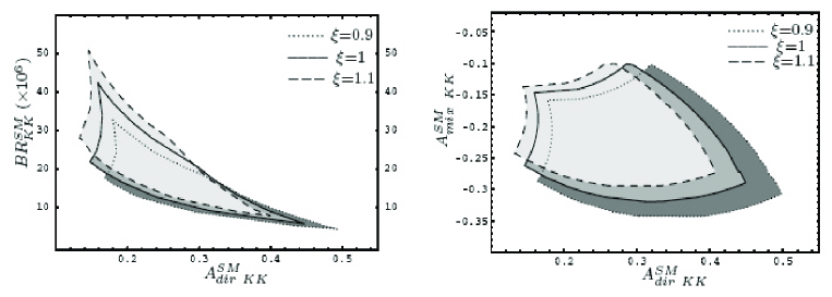
Figure 4.6: Correlations between the observables $A_{dir\ \scriptscriptstyle KK}^{\scriptscriptstyle SM}-BR^{\scriptscriptstyle SM}_{\scriptscriptstyle KK}$ and $A_{dir\ \scriptscriptstyle KK}^{\scriptscriptstyle SM}-A_{mix\ \scriptscriptstyle KK}^{\scriptscriptstyle SM}$, for $\gamma=61^{\circ}$ and $\xi=1$, $\xi=0.9$ and $\xi=1.1$.

These results can be used as a consistency check when comparing with experiment, or can be used together with experimental data to extract the NP parameters $\mathcal{A}^{u}$, $\Phi_{u}$ and $\delta_{T}$. Up to date the only available piece of data on $B_{s}^{0}\to K^{+}K^{-}$ is the value of given by CDF [131],

$$BR(B_{s}\to K^{+}K^{-})_{\rm exp}=(24.4\pm 1.4\pm 4.6)\cdot 10^{-6}$$ (4.29)

which fits fairly good in the SM prediction, and implies a value for $\mathcal{B}^{\scriptscriptstyle\rm NP}$ compatible with zero,

$$\mathcal{B}^{\scriptscriptstyle\rm NP}\in(-0.54,3.56)$$ (4.30)

but with large errors that still allow for the presence of NP.

4.6 A glimpse further

The method described above to measure the NP parameters would rule out automatically all those NP models that fit the conditions listed in Section 4.5 but do not reproduce the measured values for these parameters. To that end one should compute the contributions coming from each particular model to be tested, which can be quite a tedious job. There are, however, several generic features of the NP flavor structure that could be identified at once by the power of flavor symmetries. All NP models which do not share these features would be ruled out.

Consider the decay $B_{s}^{0}\to K^{0}\bar{K}^{0}$. Only the diagrams (c) in Fig. 4.1 contribute to this decay, so only the penguin $P^{s}_{K^{0}\!\bar{K}^{0}}$ can be related to $P^{s}_{K^{+}\!K^{-}}$ by U-spin, and not the tree $T^{s}_{K^{0}\!\bar{K}^{0}}$ (which does not contain the “pure” tree (a)). However, because $|\lambda_{u}^{(s)}|\ll|\lambda_{c}^{(s)}|$, the amplitude for this process can be approximately written as

$$A(B_{s}^{0}\to K^{0}\bar{K}^{0})=\lambda_{c}^{(s)*}P^{s}_{K^{0}\!\bar{K}^{0}}+\mathcal{A}^{d}e^{i\Phi_{d}}$$ (4.31)

Then measurements on $B_{s}^{0}\to K^{0}\bar{K}^{0}$ allow to extract the NP parameters $\mathcal{A}^{d}$ and $\Phi_{d}$.

Consider the case in which the NP is isospin conserving. This means that whatever this NP is, it should predict $\mathcal{A}^{d}=\mathcal{A}^{u}$ and $\Phi_{d}=\Phi_{u}$. Now, if the measured values for the NP parameters do not fit this rule, then all isospin conserving NP models can be discarded.

The main advantage of using experimental measurements on a particular decay together with flavor symmetries to extract information in other channels, is that the hadronic effects are taken into account in a model independent way. The price we pay is the large uncertainties coming from the SU(3) breaking effects (up to 30%), which are still not under control.

A different approach is to use a particular theoretical framework to calculate the matrix elements, but the inclusion of hadronic effects always leads to model dependence. It would be a step forward if both approaches could be combined to reach more reliable predictions.

An attempt in this direction has been made in [36] using QCDF. According to the discussion at the end of Section 2.1.4, and as will be explained in detail in Chapter 5, the quantity

$$\Delta\ \equiv\ T^{d}_{K^{0}\!\bar{K}^{0}}-P^{d}_{K^{0}\!\bar{K}^{0}}$$ (4.32)

for the decay $B_{d}^{0}\to K^{0}\bar{K}^{0}$, is free from infrared divergencies when computed using QCDF. From (4.32) and the measured values for the branching ratio and the direct CP-asymmetry for this decay, one can obtain its hadronic parameters $T^{d}_{K^{0}\!\bar{K}^{0}}$ and $P^{d}_{K^{0}\!\bar{K}^{0}}$. QCDF predicts a relationship between these and the hadronic parameters for $B_{s}^{0}\to K^{+}K^{-}$, which is now free of most of the model dependence, and thus much more reliable than the pure QCDF computation.

As an example, one can obtain $d^{s}_{K^{+}\!K^{-}}$ in this way, and together with $d^{d}_{\pi^{+}\pi^{-}}$ from Table 4.1 obtain a value for the U-spin breaking parameter $\xi$. This is described in detail in Chapter 5. The result as given in ref. [36] is

$$\xi=0.81\pm 0.35$$ (4.33)

This value can then be used in the analysis of Section 4.5 instead of the poorly justified one taken above. However, one should consider carefully up to what point these two approaches are independent when using the value in eq. (4.33) for $\xi$.

Chapter 5 Exploring $B\to KK$ Decays with Flavor Symmetries and QCDF

Along the past chapters of this thesis we have seen continuously the difficulty and the phenomenological importance of the computation of the hadronic parameters (“tree” and “penguin”) in two body non-leptonic $B$ decays. We have seen that this type of decays contain a huge amount of information that can be used to understand and test the SM and to look and measure NP; but we have also seen that in order to do that the effects of strong interactions have to be controlled in some way.

Moreover, the increasing precision that is being achieved experimentally, and the optimistic prospects for the future coming from the successes of the CDF collaboration, the starting of LHC, and the possibility of a Super-B, urges the development of theoretical tools improving on the treatment of hadronic uncertainties.

We have already seen several ways in which hadronic parameters in two-body non-leptonic $B$ decays can be extracted. First, in Section 4.2 we have seen how these can be extracted directly from data. The argument is that three hadronic parameters can be extracted from three independent observables, which for neutral $B$ decays are the branching ratio and the two components of the time dependent CP asymmetry. One just has to invert the equations (4.8)-(4.10) and solve for the hadronic parameters. For the case of $B_{d}\to\pi^{+}\pi^{-}$, the results were given in Table 4.1. One should be careful, though, when using this procedure in NP analyses, since this is only correct when the decay at hand is not affected by the NP. In this thesis we bypass this potential problem by assuming that any NP affecting $\bar{b}\to\bar{d}$ transitions is negligible at the considered level of accuracy.

A second approach that may be used to extract the hadronic parameters is QCDF as outlined in Sections 2.1.3 and 2.1.4. The amplitude of a $B$ decay in QCDF is given by the matrix elements in eq. (2.43). Therefore, the hadronic parameters are given by $T_{\scriptscriptstyle M_{1}M_{2}}=\langle M_{1}M_{2}|\mathcal{T}_{A}^{u}+\mathcal{T}_{B}^{u}|B\rangle$ and $P_{\scriptscriptstyle M_{1}M_{2}}=\langle M_{1}M_{2}|\mathcal{T}_{A}^{c}+\mathcal{T}_{B}^{c}|B\rangle$ (see Section 2.1.4). For the $B_{d}\to\pi^{+}\pi^{-}$ example, the hadronic parameters predicted by QCDF are shown in Table 5.1 [27]. The corresponding QCDF prediction for the $B_{d}\to\pi^{+}\pi^{-}$ branching ratio is

$$BR(B_{d}\to\pi^{+}\pi^{-})_{\rm\scriptscriptstyle QCDF}=8.9^{+4.0}_{-3.4}\,{}^{+3.6}_{-3.0}\,{}^{+0.6}_{-1.0}\,{}^{+1.2}_{-0.8}\times 10^{-6}$$ (5.1)

which gives a central value which is high compared to the experimental number (4.11), but with tremendous uncertainties. Clearly this is presently a problematic decay for the QCDF approach.

	Theory	S2	S3	S4
$|T_{\pi\pi}|\ (10^{-6}{\rm GeV})$	$7.7^{+0.04}_{-0.06}$	6.3	7.8	6.8
$|P_{\pi\pi}/T_{\pi\pi}|$	$0.32^{+0.16}_{-0.09}$	0.49	0.37	0.48

Table 5.1: Hadronic parameters for $B_{d}\to\pi^{+}\pi^{-}$ from QCDF. S2, S3 and S4 correspond to different scenarios for the inputs as described in ref. [27].

An alternative way to extract the hadronic parameters with the aim of giving predictions for the observables, is the flavor symmetry analysis described in Section 4.5. The process consists in establishing $SU(3)$ relations between the hadronic parameters such that the knowledge of some hadronic parameters (that are extracted from data) allows to know the other hadronic parameters on which we are interested. Then, after a sensible inclusion of $SU(3)$ breaking effects, one can calculate observables. The analysis in Chapter 4 relating $B_{d}\to\pi^{+}\pi^{-}$ and $B_{s}\to K^{+}K^{-}$ gave the predictions plotted in Fig. 4.6.

A comparative plot between the predictions for $B_{s}\to K^{+}K^{-}$ from QCDF and flavor symmetry is shown in Fig. 5.1. As can be seen, the theoretical predictions have uncertainties much above the experimental precision. Moreover, this decay will probably be measured with better accuracy in Tevatron shortly, including the direct CP asymmetry. In LHCb both observables will be measured with very high accuracy. Therefore, it is mandatory to improve substantially the theoretical predictions if the experimental efforts want to be exploited. But, how can this be done? To answer this question it is necessary to understand what are the advantages and limitations of each of these approaches.

\psfrag{aa}{\tiny$\xi=0.8$}\psfrag{bb}{\tiny$\xi=1.0$}\psfrag{cc}{\tiny$\xi=1.2$}\psfrag{dd}{\tiny QCDF}\psfrag{ee}{\tiny CDF}\psfrag{BR}{\small $\stackrel{{\scriptstyle BR(B_{s}^{0}\to K^{+}K^{-})\times 10^{6}}}{{}}$}\psfrag{Adir}{\begin{minipage}[l]{199.16928pt}\vspace{0.5cm}{\tiny$A_{dir}(B_{s}^{0}\to K^{+}K^{-})$}\end{minipage}}\includegraphics[height=170.71652pt,width=284.52756pt]{ComparativeBKK.eps}

Figure 5.1: Comparison between the predictions for $B_{s}\to K^{+}K^{-}$ from QCD factorization and flavor symmetry. The green box shows the QCDF prediction [27] (errors summed in quadrature), the gray regions show the predictions using $B_{d}\to\pi^{+}\pi^{-}$ and flavor symmetry for different amounts of $SU(3)$ breaking (c.f. Chapter 4), and the blue horizontal line is the experimental value for the branching ratio [132].

The flavor-symmetry approach has several positive features. It is a model-independent approach based on symmetries of the QCD lagrangian alone, as described in Section 2.2. It also includes all the hadronic long-distance effects naturally, since they are contained inside the hadronic parameters that are extracted from data. However, the major drawback is the inclusion of $SU(3)$ breaking corrections, which are obviously completely unaccessible within the framework. These symmetry breaking effects depend on the dynamics and computing them requires the use of non-perturbative methods. Alternatively, one might just assume that these effects are smaller than a certain percentage, and allow for arbitrary breaking of this size. However, even in the cases in which this can be done model-independently, the associated uncertainties that are generated preclude any precision in the predictions. Moreover, the predictions are also affected by large uncertainties related to the fact that the used data has often large experimental errors. Therefore, the flavor-symmetry approach requires of two ingredients: more accurate experimental data, and more reliable estimates of $SU(3)$ breaking.

On the other hand, QCD factorization is a purely theoretical framework based on QCD and the heavy-quark expansion. In principle its predictions are unlimited up to a particular order in $\alpha_{s}$ and $\Lambda_{\rm\scriptscriptstyle QCD}/m_{b}$. This means that it can predict all the hadronic parameters (not only those for which a flavor-symmetry relation can be found) provided the non-perturbative input of form factors, decay constants and LCDAs is given. However, as discussed at the end of Section 2.1.4, there are some difficulties with non-factorizable $1/m_{b}$ corrections that are numerically relevant because they are chirally enhanced. When including these corrections, the infrared divergencies must be subtracted in a model-dependent way, and the predictive power is partially lost. Moreover, as was already commented in Section 2.1.4, in QCDF the strong phases are perturbatively calculable, and therefore appear first at order $\alpha_{s}$, which means that they are in general predicted to be small. Phenomenologically, however, there are certain decays (for example $B\to\pi\pi$) in which the strong phases could be large, and not accountable by a $\mathcal{O}(\alpha_{s})$ correction. The QCD factorization approach should then be provided with a prescription to control the phenomenologically relevant power-suppressed infrared divergencies, and with a mechanism that generates large strong phases whenever they are there.

In this chapter we present an approach that improves (at a phenomenological level) on the weak points mentioned above. This approach was proposed in [36] and since then it has been applied in [37, 38, 39, 40].

5.1 The theoretical input: $\Delta$

We consider now the following quantity defined as the difference between tree and penguin contributions,

$$\Delta\equiv T-P\ .$$ (5.2)

This quantity is a hadronic, process-dependent, intrinsically non-perturbative object, and thus difficult to compute theoretically. Such hadronic quantities are usually either extracted from data or computed using some factorization-based approach, according to the long discussion given above. In the latter case, $\Delta$ could suffer from the aforementioned phenomenological problems of factorization.

However, for a certain class of decays, $T$ and $P$ share the same long-distance dynamics: the difference comes from the ($u$ or $c$) quark running in the loop, which is dominated by short-distance physics [36]. Indeed, in such decays, $\Delta=T-P$ is not affected by the breakdown of factorization that affects annihilation and hard-spectator contributions, and it can be computed in a well-controlled way leading to safer predictions and smaller uncertainties.

Consider first the effect of the $A$-operators in eq. (LABEL:Aops). The contribution to $\Delta$ will come from $\mathcal{T}_{A}^{u}-\mathcal{T}_{A}^{c}$. The current-current pieces will be just $\sim a_{1}(\cdots)+a_{2}(\cdots)$ since they only appear in $\mathcal{T}_{A}^{u}$. They will be proportional to the hard spectator functions $H_{1}$ and $H_{2}$ and they will be affected by the already familiar IR divergencies. However, the rest of the pieces will be $\sim(a_{i}^{u}-a_{i}^{c})$. So looking at eq. (2.57) we see that they will just receive contributions from the penguin contributions, proportional to the functions $(P_{i}^{u}-P_{i}^{c})$. These functions are well behaved, and dominated by short-distance physics. At order $\alpha_{s}$, and neglecting electromagnetic corrections, penguin contractions are only present for $i=4,6$, so the only contribution to $\Delta$ (besides the $a_{1}$ and $a_{2}$ part) will be proportional to $\ (P_{4}^{u}-P_{4}^{c})\pm r_{\chi}(P_{6}^{u}-P_{6}^{c})$. Specifically, (see ref. [27]) we have

$$P_{4}^{u}(M_{2})-P_{4}^{c}(M_{2}) = -\frac{C_{F}\alpha_{s}}{4\pi N_{c}}\,C_{1}\Big{[}G_{\scriptscriptstyle M_{2}}(0)-G_{\scriptscriptstyle M_{2}}(m_{c}^{2}/m_{b}^{2})\Big{]}\ ,$$

$$P_{6}^{u}(M_{2})-P_{6}^{c}(M_{2}) = -\frac{C_{F}\alpha_{s}}{4\pi N_{c}}\,C_{1}\Big{[}\hat{G}_{\scriptscriptstyle M_{2}}(0)-\hat{G}_{\scriptscriptstyle M_{2}}(m_{c}^{2}/m_{b}^{2})\Big{]}\ ,$$ (5.3)

where $G(x)$ and $\hat{G}(x)$ are certain penguin functions. The $B$-operators in Eq. (LABEL:Bops) contain also the pieces proportional to $b_{1}$ and $b_{2}$ that enter $\mathcal{T}_{B}^{u}$ and not $\mathcal{T}_{B}^{c}$, and these pieces will introduce the IR divergencies from weak annihilation. The rest of the pieces, however, as can be seen looking at the specific form of the coefficients $b_{i}$ [27], cancel completely in the difference $b_{i}^{u}-b_{i}^{c}$.

So now consider penguin-mediated decays that do not receive contributions from $a_{1,2}$ or $b_{1,2}$. For these decays, the quantity $\Delta$ is at $\mathcal{O}(\alpha_{s})$ free from dangerous IR divergencies in QCDF. This makes it a quantity that can be computed with acceptable accuracy and can be used as a reliable theoretical input. In general, $\Delta$ is given by

$$\Delta_{\scriptscriptstyle M_{1}M_{2}}=A_{\scriptscriptstyle M_{1}M_{2}}\frac{C_{F}\alpha_{s}}{4\pi N}C_{1}\big{[}\bar{G}_{\scriptscriptstyle M_{2}}(m_{c}^{2}/m_{b}^{2})-\bar{G}_{\scriptscriptstyle M_{2}}(0)\big{]}\ ,$$ (5.4)

where $\bar{G}_{\scriptscriptstyle M_{2}}\equiv G_{\scriptscriptstyle M_{2}}\pm r_{\chi}^{\scriptscriptstyle M_{2}}\hat{G}_{\scriptscriptstyle M_{2}}$, with the plus or the minus sign depending on whether $M_{1}$ is a pseudoscalar or a vector meson.

In our analysis of $B\to KK$ modes, we are mainly interested in $\Delta^{d}_{\scriptscriptstyle KK}$ corresponding to $B_{d}\to K^{0}\bar{K}^{0}$. A careful computation gives

$$|\Delta^{d}_{\scriptscriptstyle KK}|=(2.96\pm 0.97)\times 10^{-7}\ .$$ (5.5)

Only the absolute value is physical, because an unphysical global phase in the amplitude would rotate simultaneously $P$ and $T$, rotating $\Delta$ accordingly. In particular, in the formulae for the hadronic parameters given in the following section, $\Delta$ can be chosen to be real, introducing only a global phase in the amplitude. From now on we will always take it as a real quantity. The values of the inputs used in the numerical evaluation of $\Delta^{d}_{\scriptscriptstyle KK}$, and the impact of each one of them on the error, are given in tables 5.2 and 5.3.

$\mu$	$\alpha_{1}^{K}$	$\alpha_{2}^{K}$	$F^{B\to K}_{0}$	$m_{s}(2\,{\rm GeV})$	$m_{c}/m_{b}$
$(m_{b}/2,2m_{b})$	$0.2\pm 0.2$	$0.1\pm 0.3$	$0.34\pm 0.05$	$103\pm 20$ MeV	$0.30\pm 0.06$

Table 5.2: Inputs used in the computation of $\Delta^{d}_{\scriptscriptstyle KK}$.

	$\mu$	$\alpha_{1}^{K}$	$\alpha_{2}^{K}$	$F^{B\to K}_{0}$	$m_{s}(2\,{\rm GeV})$	$m_{c}/m_{b}$
$|\Delta^{d}_{\scriptscriptstyle KK}|$	$19.7\%$	$4.1\%$	$0.9\%$	$15.8\%$	$5.7\%$	$53.7\%$

Table 5.3: Relative impact of the input uncertainties on the error of $\Delta^{d}_{\scriptscriptstyle KK}$.

5.2 Tree and Penguin contributions

We now describe how to obtain the hadronic parameters $T$ and $P$ from $\Delta$ and experimental data. The derivation will be completely general, and is valid for any decay, independently of whether the computation of $\Delta$ is theoretically clean or not. We begin writing the two self-conjugated amplitudes in terms of tree and penguin contributions,

$$A=\lambda_{u}^{(D)*}T+\lambda_{c}^{(D)*}P\ ,\quad\bar{A}=\lambda_{u}^{(D)}T+\lambda_{c}^{(D)}P\ .$$ (5.6)

Now we put $T=P-\Delta$ and we square the amplitudes,

$$\begin{array}[]{rcl}|A|^{2}&=&|\lambda_{c}^{(D)*}+\lambda_{u}^{(D)*}|^{2}\left|P+\frac{\lambda_{u}^{(D)*}}{\lambda_{c}^{(D)*}+\lambda_{u}^{(D)*}}\Delta\right|^{2}\ ,\\ &&\\ |\bar{A}|^{2}&=&|\lambda_{c}^{(D)}+\lambda_{u}^{(D)}|^{2}\left|P+\frac{\lambda_{u}^{(D)}}{\lambda_{c}^{(D)}+\lambda_{u}^{(D)}}\Delta\right|^{2}\ .\end{array}$$ (5.7)

But the squared amplitudes are directly related to observables,

$$|A|^{2} = BR(1+\mathcal{A}_{\rm dir})/g_{PS}\ ,$$

$$|\bar{A}|^{2} = BR(1-\mathcal{A}_{\rm dir})/g_{PS}\ ,$$ (5.8)

where $g_{PS}$ is the usual phase-space factor (c.f. Eq. (6.5)). So two equations can be written that relate observables with $P$ and $\Delta$,

$$\frac{BR(1+\mathcal{A}_{\rm dir})/g_{PS}}{|\lambda_{c}^{(D)*}+\lambda_{u}^{(D)*}|^{2}}=\left|P+\frac{\lambda_{u}^{(D)*}}{\lambda_{c}^{(D)*}+\lambda_{u}^{(D)*}}\Delta\right|^{2}\ ,$$

$$\frac{BR(1-\mathcal{A}_{\rm dir})/g_{PS}}{|\lambda_{c}^{(D)}+\lambda_{u}^{(D)}|^{2}}=\left|P+\frac{\lambda_{u}^{(D)}}{\lambda_{c}^{(D)}+\lambda_{u}^{(D)}}\Delta\right|^{2}\ .$$ (5.9)

These are the equations for two circles in the complex $P$ plane, whose solutions are the two points of intersection. This will result in a two-fold ambiguity in the determination of $P$ and $T$ (see Fig. 5.2). Before writing down the analytical solutions, notice that in order for solutions to exist, the separation between the centers of these circles must be smaller than the sum of the radii but bigger than the difference. This translates into a consistency condition between $BR$, $\mathcal{A}_{\rm dir}$ and $\Delta$:

$$|\mathcal{A}_{\rm dir}| \leq \sqrt{\frac{\mathcal{R}_{D}^{2}\Delta^{2}}{2\widetilde{BR}}\Big{(}2-\frac{\mathcal{R}_{D}^{2}\Delta^{2}}{2\widetilde{BR}}\Big{)}}\approx\frac{\mathcal{R}_{D}\Delta}{\sqrt{\widetilde{BR}}}\ ,$$

$$\widetilde{BR} \geq \frac{\mathcal{R}_{D}^{2}\Delta^{2}}{4}\ ,$$ (5.10)

where $\widetilde{BR}\equiv BR/g_{PS}\$, and $\mathcal{R}_{D}$ is a specific combination of CKM factors, $\mathcal{R}_{D}=2|c_{0}^{\scriptscriptstyle(D)}|/\sqrt{c_{2}^{\scriptscriptstyle(D)}}$ (see below). The approximation for the upper bound on $|\mathcal{A}_{\rm dir}|$ holds up to very small corrections in the usual situation $\Delta\lesssim\mathcal{O}(10^{-7})$ and $BR\sim\mathcal{O}(10^{-6})$. The first condition in eq. (5.10) turns out to be highly nontrivial. For example, Fig. 5.3 shows the allowed values for the direct CP asymmetry of $B_{d}\to K^{0}\bar{K}^{0}$ in terms of its branching ratio. It can be seen that for the present data of the branching ratio, the direct CP asymmetry is predicted to be less than about $\sim 20\%$.

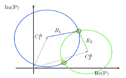
Figure 5.2: Eqs. (5.9) can be written as $R_{1}=|P-C_{1}^{\Delta}|$ and $R_{2}=|P-C_{2}^{\Delta}|$, where the $R_{i}$ depend only on data and CKM elements, and the $C_{i}^{\Delta}$ depend only on $\Delta$ and CKM elements. These are the equations for two circles with centers in $C_{i}^{\Delta}$ and radii $R_{i}$ in the complex $P$ plane. Their crossing points are the solutions for $P$. The condition for the existence of solutions is $|R_{1}-R_{2}|\leq|C_{1}^{\Delta}-C_{2}^{\Delta}|\leq|R_{1}+R_{2}|$, which translates into Eqs. (5.10).

\psfrag{A}{$\mathcal{A}_{\rm dir}(B_{d}\to K^{0}\bar{K}^{0})$}\psfrag{BR}{$BR(B_{d}\to K^{0}\bar{K}^{0})\times 10^{6}$}\includegraphics[width=227.62204pt]{BRvsAdir.eps}

Figure 5.3: Allowed values for the direct CP asymmetry of $B_{d}\to K^{0}\bar{K}^{0}$ in terms of its branching ratio, according to the value of $\Delta_{KK}^{d}$. The vertical blue band corresponds to the experimental branching ratio, which sets an upper bound on $|\mathcal{A}_{\rm dir}|$ slightly above $0.2$.

The hadronic quantities $P$ and $T$ are then given by

$$Im[P] = \frac{\widetilde{BR}\,\mathcal{A}_{\rm dir}}{2c_{0}^{(D)}\Delta}\ ,$$

$$Re[P] = -c_{1}^{(D)}\,\Delta\pm\sqrt{-Im[P]^{2}-\left(\frac{c_{0}^{(D)}\Delta}{c_{2}^{(D)}}\right)^{2}+\frac{\widetilde{BR}}{c_{2}^{(D)}}}\ ,$$

$$T = P+\Delta\ ,$$ (5.11)

where the coefficients $c_{i}^{(D)}$ are again some specific combinations of CKM elements (see Table 5.4).

$c_{0}^{(d)}$	$c_{1}^{(d)}$	$c_{2}^{(d)}$	$\mathcal{R}_{d}$
$\ -3.15\cdot 10^{-5}\$	$\ -0.034\$	$\ 6.93\cdot 10^{-5}\$	$7.58\cdot 10^{-3}$
$c_{0}^{(s)}$	$c_{1}^{(s)}$	$c_{2}^{(s)}$	$\mathcal{R}_{s}$
$\ 3.11\cdot 10^{-5}\$	$\ 0.011\$	$\ 1.63\cdot 10^{-3}\$	$1.54\cdot 10^{-3}$

Table 5.4: Numerical values for the coefficients $c_{i}^{(D)}$ and $\mathcal{R}_{D}$ for $\gamma=62^{\circ}$.

Equations (5.11) allow to extract the hadronic parameters $T$ and $P$ from experimental data on $BR$ and $\mathcal{A}_{\rm dir}$, information on sides of the unitarity triangle and the weak phase $\gamma$, and the theoretical value for $\Delta$. This method is also powerful because if no experimental information is available for $\mathcal{A}_{\rm dir}$, one can just vary $\mathcal{A}_{\rm dir}$ over its allowed range in eq.(5.10). So in fact $T$ and $P$ can be extracted from $BR$, $\Delta$ and CKM elements. This is just the case for $B_{d}\to K^{0}\bar{K}^{0}$: while there is a preliminary experimental number for the direct CP asymmetry, it is still too uncertain. Therefore, in our analysis we will assume that $\mathcal{A}_{\rm dir}(B_{d}\to K^{0}\bar{K}^{0})$ is unknown, and we will give results for different values of this asymmetry between $-0.2$ and $0.2$, according to Fig. 5.3. We will also see that this range can be still made smaller by looking at data on $B_{d}\to\pi^{+}\pi^{-}$, but this will not be taken into account in our analysis.

Finally, we would like to mention that this procedure is also useful to extract hadronic parameters from charged $B$ decays, were the CP observables are just two: branching ratio and CP asymmetry. An example is the decay $B^{+}\to\pi^{+}\phi$, for which the very small value $\Delta_{\pi^{+}\phi}\sim 10^{-8}\$ indicates a very small CP asymmetry, as long as the branching ratio is not too small (at present there is only an upper bound).

5.3 Flavor symmetries and QCDF

Using $U$-spin symmetry, we can relate the two penguin-mediated decays $\bar{B}_{d}\to K_{0}\bar{K}_{0}$ and $\bar{B}_{s}\to K_{0}\bar{K}_{0}$, as exemplified in fig. 5.4. Let us stress that we work with the operators of the effective Hamiltonian: internal loops have already been integrated out to yield four-quark operators, so that the internal loop of the $u$-penguin is not affected by $U$-spin rotations. $U$-spin breaking should be much smaller here than usual: it does not affect final-state interaction since both decays involve the same outgoing state, and it shows up mainly in power-suppressed effects. This is confirmed by QCDF:

$$P^{s0} = f\,P^{d0}\Big{[}1+(A^{d}_{\scriptscriptstyle KK}/P^{d0})\Big{\{}\delta\alpha_{4}^{c}+\delta\beta_{3}^{c}+2\delta\beta_{4}^{c}\Big{\}}\Big{]}\ \equiv\ f\,P^{d0}\,(1+\delta_{P^{s0}})\,,$$

$$T^{s0} = f\,T^{d0}\Big{[}1+(A^{d}_{\scriptscriptstyle KK}/T^{d0})\Big{\{}\delta\alpha_{4}^{u}+\delta\beta_{3}^{u}+2\delta\beta_{4}^{u}\Big{\}}\Big{]}\ \equiv\ f\,T^{d0}\,(1+\delta_{T^{s0}})\,,$$ (5.12)

where we define the $U$-spin breaking differences $\delta\alpha_{i}^{p}\equiv\bar{\alpha}_{i}^{p}-\alpha_{i}^{p}$ (id. for $\beta$). The superscripts identify the channel and the bar denotes quantities for decays with a spectator $s$ quark. Apart from the factorizable ratio :

$$f=\frac{A_{\scriptscriptstyle KK}^{s}}{A_{\scriptscriptstyle KK}^{d}}=\frac{M_{B_{s}}^{2}F_{0}^{\bar{B}_{s}\to K}(0)}{M_{B_{d}}^{2}F_{0}^{\bar{B}_{d}\to K}(0)}=0.94\pm 0.20$$ (5.13)

which should be computed on the lattice, $U$-spin breaking arises through $1/m_{b}$-suppressed contributions in which most long-distance contributions have cancelled out.

First, the hard-spectator scattering ($\delta\alpha$) probes the difference between $B_{d}$- and $B_{s}$-distribution amplitudes:

$$\delta\alpha_{4}^{p} = \alpha_{s}C_{F}C_{3}\pi/N_{c}^{2}\times\delta\lambda_{B}\times[\langle\bar{x}\rangle_{\scriptscriptstyle K}^{2}+r_{\chi}^{\scriptscriptstyle K}\langle x\rangle_{\scriptscriptstyle K}X_{H}^{\scriptscriptstyle K}]\ ,$$

$$\delta\lambda_{B} = B_{\scriptscriptstyle KK}^{s}M_{B_{s}}/(A_{\scriptscriptstyle KK}^{s}\lambda_{B_{s}})-B_{\scriptscriptstyle KK}^{d}M_{B_{d}}/(A_{\scriptscriptstyle KK}^{d}\lambda_{B_{d}})\ ,$$ (5.14)

$B_{\scriptscriptstyle KK}^{q}=f_{B_{q}}f_{K}^{2}{G_{F}}/{\sqrt{2}}$, $\langle\bar{x}\rangle_{K}$ and $M_{B_{q}}/\lambda_{B_{q}}$ are first and first inverse moments of $K$ and $B_{q}$ distribution amplitudes [27], respectively. $\delta\lambda_{B}$ is expected small, since the dynamics of the heavy-light meson in the limit $m_{b}\to\infty$ should vary little from $B_{d}$ and $B_{s}$. Second, the annihilation contributions ($\delta\beta$) contain a $U$-spin breaking part when the gluon is emitted from the light quark in the $B_{d,s}$-meson (this effect from $A_{1}^{i}$ and $A_{2}^{i}$ defined in [27] is neglected in the QCDF model for annihilation terms).

Taking the hadronic parameters in [27], we obtain

$$|\delta_{P^{s0}}|\leq 0.03\ ,\quad|\delta_{T^{s0}}|\leq 0.03\ .$$ (5.15)

These relations yield also the constraint $\Delta^{s}_{\scriptscriptstyle KK}=f\Delta^{d}_{\scriptscriptstyle KK}$ up to $1/m_{b}$-suppressed corrections, relating observables in both decays.

(-329,44)[lb]$B_{d}^{0}$ (-212,15)[lb]$K^{0}$ (-210,78)[lb]$\bar{K}^{0}$ (-300,54)[lb]$\bar{b}$ (-265,29)[lb]$d$ (-235,73)[lb]$\bar{d}$ (-223,60)[lb]$s$ (-223,33)[lb]$\bar{s}$ (-275,-5)[lb]$(a)$ (-136,44)[lb]$B_{s}^{0}$ (-20,15)[lb]$\bar{K}^{0}$ (-21,78)[lb]$K^{0}$ (-110,55)[lb]$\bar{b}$ (-70,27)[lb]$s$ (-33,33)[lb]$\bar{d}$ (-30,60)[lb]$d$ (-42,75)[lb]$\bar{s}$ (-75,-5)[lb]$(b)$ (-82,46)[lb]$\bar{u},\!\bar{c},\!\bar{t}$

Figure 5.4: Diagrams contributing to (a) $B_{d}\to K^{0}\bar{K}^{0}$ and (b) $B_{s}\to K^{0}\bar{K}^{0}$ related through a $U$-spin transformation.

Relations exist between $\bar{B}_{d}\to K_{0}\bar{K}_{0}$ and $\bar{B}_{s}\to K^{+}K^{-}$ as well. A combination of $U$-spin and isospin rotations leads from the penguin contribution in $\bar{B}_{d}\to K_{0}\bar{K}_{0}$ to that in $\bar{B}_{s}\to K_{0}\bar{K}_{0}$, then to $\bar{B}_{s}\to K^{+}K^{-}$, up to electroweak corrections (it corresponds to fig. 5.4 up to replacing $d\to u$ in the right-hand diagram). On the other hand, there are no such relations between tree contributions, since $\bar{B}_{s}\to K^{+}K^{-}$ contains tree contributions which have no counterpart in the penguin-mediated decay $\bar{B}_{d}\to K_{0}\bar{K}_{0}$. This is seen in QCDF as well:

$$P^{s\pm} = f\,P^{d0}\Big{[}1+({A_{\scriptscriptstyle KK}^{d}}/{P^{d0}})\Big{\{}\frac{3}{2}(\delta\alpha_{4}^{c}+\delta\beta_{3}^{c}+2\delta\beta_{4}^{c}\Big{\}}\Big{]}\,\equiv\,f\,P^{d0}\,(1+\delta_{P^{s\pm}})\ ,$$ (5.16)

$$T^{s\pm} = f\,T^{d0}+A^{s}_{\scriptscriptstyle KK}{\bar{\alpha}_{1}}\Big{[}1+\frac{1}{\bar{\alpha}_{1}}\Big{\{}\bar{\beta}_{1}+\delta\alpha_{4}^{u}+\delta\beta_{3}^{u}+2\delta\beta_{4}^{u}\Big{\}}\Big{]}\,\equiv\,f\,T^{d0}+A^{s}_{\scriptscriptstyle KK}{\bar{\alpha}_{1}}\,(1+\delta_{T^{s\pm}})\ .$$

From QCDF, we obtain the following bounds:

$$|\delta_{P^{s\pm}}|\leq 0.02\ ,\quad|\delta_{T^{s\pm}}|\leq 0.04\ .$$ (5.17)

The latter bound shows that the flavor-symmetry breaking corrections are smaller than $\ T^{d0}/(A^{d}_{\scriptscriptstyle KK}\bar{\alpha}_{1})=O(10\%)$. Fortunately, $T^{s\pm}$ is strongly CKM suppressed in $B_{s}\to K^{+}K^{-}$ so that the uncertainty on its QCDF determination will affect the branching ratio and CP-asymmetries only marginally.

Finally, these relations between $B_{d}$ and $B_{s}$ hadronic parameters are affected by electroweak penguins, small in the SM but potentially enhanced by NP effects.

5.4 SM predictions for $B_{s}\to KK$ and SU(3) breaking

In this section we present the results for the branching ratios and CP asymmetries of $B_{s}\to K^{0}\bar{K}^{0}$ and $B_{s}\to K^{+}K^{-}$. The knowledge of the $B_{s}\to K^{+}K^{-}$ hadronic parameters, which require data from $B_{d}\to K^{0}\bar{K}^{0}$ (and not $B_{d}\to\pi^{+}\pi^{-}$ as in Chapter 4) allows us to give also predictions for the $SU(3)$ breaking parameters $|r_{T}|$ and $\xi$ used in Chapter 4 relating $B_{s}\to K^{+}K^{-}$ to $B_{d}\to\pi^{+}\pi^{-}$.

Let us outline briefly the basic steps in the process.

• The $B_{d}\to K^{0}\bar{K}^{0}$ hadronic parameters $P^{d0}$ and $T^{d0}$ are obtained from Eqs. (5.11), with the value of $\Delta^{d}_{\scriptscriptstyle KK}$ given in Eq. (5.5) and the experimental value for the $B_{d}\to K^{0}\bar{K}^{0}$ branching ratio [133]

  $$BR(B_{d}\to K^{0}\bar{K}^{0})_{\rm exp}=(1.08\pm 0.30)\cdot 10^{-6}\ .$$ (5.18)

  Since the $B_{d}\to K^{0}\bar{K}^{0}$ direct CP asymmetry ($A^{d0}_{\rm dir}$) is still uncertain, we vary its value between $-0.2$ and $0.2$ according to the discussion in Section 5.2 (see Fig. 5.3).

• The hadronic parameters $P^{s0}$, $T^{s0}$, $P^{s\pm}$ and $T^{s\pm}$ for $B_{s}\to K^{0}\bar{K}^{0}$ and $B_{s}\to K^{+}K^{-}$ are obtained as described in Section 5.3, in particular from Eqs. (5.12), (5.16), (5.15) and (5.17). In order to account for well-behaved short-distance $1/m_{b}$-suppressed corrections not yet included, we stretch the $SU(3)$ breaking bounds to more conservative ranges:

  $$|\delta_{P^{s0}}|,\,|\delta_{T^{s0}}|,\,|\delta_{P^{s\pm}}|,\,|\delta_{T^{s\pm}}|\leq 0.05\ .$$ (5.19)

  This $\delta$’s are complex quantities and their phases are varied from $0$ to $2\pi$.

• The observables are then obtained from the ranges of the hadronic parameters.

There is a further comment before presenting the results. We already mentioned in Section 5.2 that the extraction of the hadronic parameters results in a two-fold ambiguity (see Fig. 5.2). We lift this ambiguity on the basis that the rejected predictions would be in conflict with the $B_{d}\to\pi^{+}\pi^{-}$ analysis made in Chapter 4: First, this solution requires a way too large $U$-spin breaking in $\arg(P/T)$. Second, a prediction of the rejected solution is that $A_{\rm dir}^{s\pm}<0$, which is clearly in contradiction with the $B_{d}\to\pi^{+}\pi^{-}$ analysis, that predicts it positive (see Fig. 4.6).

	$BR^{s0}\,\times 10^{6}$	$A_{dir}^{s0}\,\times 10^{2}$	$A_{mix}^{s0}\,\times 10^{2}$
$A_{dir}^{d0}=-0.2$	$20.8\pm 6.7\pm 4.6\pm 1.6$	$0.9\pm 0.3\pm 0.1$	$-0.2\pm 0.8\pm 0.1$
$A_{dir}^{d0}=-0.1$	$20.6\pm 7.5\pm 4.6\pm 1.6$	$0.4\pm 0.3\pm 0.0$	$-0.7\pm 0.8\pm 0.1$
$A_{dir}^{d0}=0$	$20.5\pm 7.5\pm 4.5\pm 1.5$	$0.0\pm 0.3\pm 0.0$	$-0.8\pm 0.6\pm 0.1$
$A_{dir}^{d0}=0.1$	$20.6\pm 7.6\pm 4.5\pm 1.6$	$-0.4\pm 0.3\pm 0.0$	$-0.7\pm 0.8\pm 0.1$
$A_{dir}^{d0}=0.2$	$20.8\pm 7.0\pm 4.6\pm 1.8$	$-0.9\pm 0.3\pm 0.1$	$-0.2\pm 0.7\pm 0.2$

Table 5.5: Observables for $B_{s}\to K^{0}\bar{K}^{0}$ as functions of the direct asymmetry $A_{\rm dir}(B_{d}\to K^{0}\bar{K}^{0})$ within the SM. The errors for the branching ratios are split in: (1) Uncertainties of all inputs except $f$ and $\gamma$, (2) Uncertainty of $f$, (3) Uncertainty of $\gamma$. For the asymmetries, the second error is due to $\gamma$. The preferred values for $A_{\rm dir}^{d0}$ are highlighted (see the text).

In Table 5.5 we present the results for the $B_{s}\to K^{0}\bar{K}^{0}$ observables. An average over all the values for $A_{\rm dir}^{d0}$ gives a single prediction for the branching ratio,

$$BR(B_{s}\to K^{0}\bar{K}^{0})=(21\pm 8\pm 5\pm 2)\times 10^{-6}\ ,$$ (5.20)

and the following ranges for the CP asymmetries,

$$-0.011\leq A_{\rm dir}^{s0} \leq 0.011\ ,$$ (5.21)

$$-0.015\leq A_{\rm mix}^{s0} \leq 0.005\ .$$ (5.22)

In Table 5.6 we show the results for the $B_{s}\to K^{+}K^{-}$ observables. Again, a global average gives the following prediction for the branching ratio,

$$BR(B_{s}\to K^{+}K^{-})=(24\pm 9\pm 5\pm 2)\times 10^{-6}\ ,$$ (5.23)

and the following ranges for the CP asymmetries,

$$-0.22\leq A_{\rm dir}^{s\pm} \leq 0.49\ ,$$ (5.24)

$$-0.55\leq A_{\rm mix}^{s\pm} \leq 0.40\ .$$ (5.25)

The information from the $B_{d}\to\pi^{+}\pi^{-}$ analysis can also be used to chose some preferred values for $A_{\rm dir}^{d0}$ between those considered in Tables 5.5 and 5.6. Indeed, as can be seen from Table 5.6, there is a sign anticorrelation between $A_{\rm dir}^{d0}$ and $A_{\rm mix}^{s\pm}$. The analysis in Chapter 4 clearly predicts negative values for $A_{\rm mix}^{s\pm}$, which correspond, roughly, to positive values of $A_{\rm dir}^{d0}$. All these correlations between all these $B\to KK$ and $B\to\pi\pi$ modes turn out to be extremely powerful. In the tables we have highlighted the preferred results (corresponding to $A_{\rm dir}^{d0}\gtrsim 0$). With these restrictions the global averages given above get tightened, for example,

$$BR(B_{s}\to K^{+}K^{-})\to(20\pm 7\pm 4\pm 1)\times 10^{-6}\ ,$$ (5.26)

	$BR^{s\pm}\,\times 10^{6}$	$A_{dir}^{s\pm}\,\times 10^{2}$	$A_{mix}^{s\pm}\,\times 10^{2}$
$A_{dir}^{d0}=-0.2$	$24.9\pm 9.3\pm 5.0\pm 2.3$	$20.1\pm 15.7\pm 2.6$	$26.2\pm 11.5\pm 1.9$
$A_{dir}^{d0}=-0.1$	$22.1\pm 8.5\pm 4.7\pm 1.7$	$33.9\pm 13.0\pm 3.3$	$8.2\pm 15.1\pm 0.2$
$A_{dir}^{d0}=0$	$20.1\pm 7.3\pm 4.4\pm 1.2$	$35.3\pm 12.8\pm 2.8$	$-9.1\pm 15.3\pm 1.1$
$A_{dir}^{d0}=0.1$	$18.4\pm 6.8\pm 4.2\pm 0.9$	$27.3\pm 27.9\pm 2.1$	$-26.4\pm 18.4\pm 1.8$
$A_{dir}^{d0}=0.2$	$17.5\pm 6.5\pm 4.1\pm 0.9$	$0.5\pm 33.6\pm 1.4$	$-38.9\pm 14.8\pm 2.8$

Table 5.6: Observables for $B_{s}\to K^{+}K^{-}$ as functions of the direct asymmetry $A_{\rm dir}(B_{d}\to K^{0}\bar{K}^{0})$ within the SM. The errors mean the same as in Table 5.5.The preferred values for $A_{\rm dir}^{d0}$ are highlighted (see the text).

The prediction for the branching ratio in Eq. (5.23) or (5.26) can be already compared with the experimental value [131],

$$BR(B_{s}\to K^{+}K^{-})_{\rm exp}=(24.4\pm 1.4\pm 4.6)\times 10^{-6}\ ,$$ (5.27)

and fits nicely within the errors. Notice that the experimental errors are quite small. It is interesting to note that before this experimental number was released, the current experimental value was $\sim 40\times 10^{-6}$. In [36], the discrepancy between the theoretical results derived here and that high experimental number for the branching ratio led to the statement that [36] “…the data suggest a departure from the SM, to be further checked experimentally”, so these results were genuine predictions, and indeed, the ‘further experimental check’ fell right on top of the theoretical number.

The predictions for the $B_{s}\to K^{+}K^{-}$ observables can be compared to the other determinations (c.f. Fig. 5.1). This is shown in Fig. 5.5, where it can be easily seen that the improvement is substantial, specially in the prediction of the branching ratio.

\psfrag{xi}{}\psfrag{xi}{}\psfrag{xi}{}\psfrag{=}{}\psfrag{0.8}{\tiny$\xi=0.8$}\psfrag{1.0}{ \tiny$\xi=1.0$}\psfrag{1.2}{\tiny$\xi=1.2$}\psfrag{QCDFx}{\hskip 2.84544pt\tiny QCDF}\psfrag{CDF}{\hskip 2.84544pt\tiny CDF}\psfrag{DMVx}{\hskip 2.84544pt\tiny DMV}\psfrag{BR}{\small$\stackrel{{\scriptstyle BR(B_{s}^{0}\to K^{+}K^{-})\times 10^{6}}}{{}}$}\psfrag{Adir}{\begin{minipage}[l]{199.16928pt}\vspace{0.5cm}{\tiny$A_{dir}(B_{s}^{0}\to K^{+}K^{-})$}\end{minipage}}\includegraphics[height=170.71652pt,width=284.52756pt]{ComparativeBKK3.eps}

\psfrag{xi}{}\psfrag{xi}{}\psfrag{xi}{}\psfrag{=}{}\psfrag{0.8}{\tiny$\xi=0.8$}\psfrag{1.0}{ \tiny$\xi=1.0$}\psfrag{1.2}{\tiny$\xi=1.2$}\psfrag{QCDFx}{\hskip 2.84544pt\tiny QCDF}\psfrag{CDF}{\hskip 2.84544pt\tiny CDF}\psfrag{DMVx}{\hskip 2.84544pt\tiny DMV}\psfrag{BR}{\small$\stackrel{{\scriptstyle BR(B_{s}^{0}\to K^{+}K^{-})\times 10^{6}}}{{}}$}\psfrag{Adir}{\begin{minipage}[l]{199.16928pt}\vspace{0.5cm}{\tiny$A_{dir}(B_{s}^{0}\to K^{+}K^{-})$}\end{minipage}}\includegraphics[height=164.4569pt,width=56.9055pt]{Compare3.eps}

Figure 5.5: Comparison between the determinations of the $B_{s}\to K^{+}K^{-}$ branching ratio and direct CP asymmetry from flavor, QCDF and the method described in this chapter (we refer to it as DMV). This plot is an extension of Fig. 5.1, and shows how the new predictions improve considerably the situation posed at the beginning of this chapter.

Finally, we comment on how the results derived for the hadronic parameters can be used to predict the $SU(3)$ breaking parameters $|r_{T}|$ and $\xi$ connecting $B_{d}\to\pi^{+}\pi^{-}$ to $B_{s}\to K^{+}K^{-}$, introduced in Chapter 4. The point is that, once the $B_{d}\to\pi^{+}\pi^{-}$ hadronic parameters $T_{\pi\pi}^{d\pm}$ and $P_{\pi\pi}^{d\pm}$ are extracted from data as in Chapter 4, and the $B_{s}\to K^{+}K^{-}$ hadronic parameters $T^{s\pm}$ and $P^{s\pm}$ are obtained from $B_{d}\to K^{0}\bar{K}^{0}$ as described here, the $SU(3)$ breaking factors that connect them can be obtained.

To that end it is more useful to write the $B_{d}\to\pi^{+}\pi^{-}$ hadronic parameters obtained in Section 4.2, not as ranges, but as numbers with errors:

$$|T^{d\pm}_{\pi\pi}| = (5.48\pm 0.42)\times 10^{-6}\ ,$$

$$|P^{d\pm}_{\pi\pi}/T^{d\pm}_{\pi\pi}| = 0.13\pm 0.05\ .$$ (5.28)

Then Eqs. (4.26) give the values for the $SU(3)$ breaking parameters. In Table 5.7 we show the derived $B_{s}\to K^{+}K^{-}$ hadronic parameters and the corresponding predictions for the $SU(3)$ breaking parameters.

	$|T^{s\pm}|\times 10^{6}$	$|P^{s\pm}/T^{s\pm}|$	$\arg{(P^{s\pm}/T^{s\pm})}$	$|r_{T}|$	$\xi$
$A_{dir}^{d0}=-0.2$	$13.0\pm 2.4$	$0.10\pm 0.04$	$(38\pm 28)^{\circ}$	$2.4\pm 0.5$	$0.74\pm 0.40$
$A_{dir}^{d0}=-0.1$	$12.3\pm 2.6$	$0.10\pm 0.04$	$(77\pm 27)^{\circ}$	$2.2\pm 0.5$	$0.78\pm 0.41$
$A_{dir}^{d0}=0$	$11.7\pm 2.6$	$0.11\pm 0.04$	$(105\pm 25)^{\circ}$	$2.1\pm 0.5$	$0.82\pm 0.46$
$A_{dir}^{d0}=0.1$	$11.2\pm 2.6$	$0.11\pm 0.05$	$(134\pm 38)^{\circ}$	$2.0\pm 0.5$	$0.86\pm 0.51$
$A_{dir}^{d0}=0.2$	$10.8\pm 2.4$	$0.12\pm 0.06$	$(179\pm 30)^{\circ}$	$2.0\pm 0.5$	$0.90\pm 0.56$

Table 5.7: Hadronic parameters for $B_{s}\to K^{+}K^{-}$ and $U$-spin breaking parameters $|r_{T}|=|T^{s^{\pm}}/T_{\pi\pi}^{d^{\pm}}|$ and $\xi=|P^{s^{\pm}}/T^{s^{\pm}}|/|P_{\pi\pi}^{d^{\pm}}/T_{\pi\pi}^{d^{\pm}}|$, that relate $B_{s}\to K^{+}K^{-}$ and $B_{d}\to\pi^{+}\pi^{-}$.

Chapter 6 Penguin-Mediated $B\to VV$ Decays and the $B_{s}-\bar{B}_{s}$ Mixing Angle

The method presented in the previous chapter is powerful for many reasons. One of the reasons is that the theoretical input ($\Delta$) is quite clean, and it is the minimal information that one needs to obtain the hadronic parameters $T$ and $P$ without any information on the mixing-induced CP asymmetry of neutral $B$ decays. This property was used in Chapter 5 because there is still no experimental information on $A_{\rm mix}(B_{d}\to K^{0}\bar{K}^{0})$. However, because this asymmetry is the one that contains the information on the mixing angle (c.f. eq. (3.69)), this method can be used to extract the mixing angle from data, without the necessity of neglecting a part of the amplitude (see Section 3.4.2), or doing a $SU(3)$ analysis with some other modes, which probably requires the input of other mixing angles.

In this chapter we use the method developed in Chapter 5 to provide three alternative strategies to extract the $B_{s}-\bar{B}_{s}$ mixing angle $\phi_{s}$ from non-leptonic B decays into pairs of vector mesons. In particular we focus on $B_{d,s}\to K^{*0}\bar{K}^{*0},\phi\bar{K}^{*0},\phi\phi$ decays, for which the extraction of $\Delta$ is clean, according to the discussion in Section 5.1.

However, the theoretical study of $B$ decays with vector-vector final states is complicated. The main reason is the fact that transverse amplitudes do not factorize at leading order. In fact, naively one expects the transverse amplitudes to be suppressed in the heavy quark limit with respect to the longitudinal one. This works quite well, for example, for $B\to\rho\rho$, where the longitudinal polarization fraction is $\sim 95\%$. However, it does not work for some penguin mediated decays such as $B\to\phi K^{*0}$, where the measured polarization fraction is $\sim 50\%$. This has been called the polarization puzzle. It is therefore important to estimate properly these contributions when used; but because theoretically this is a challenge, we will concentrate on longitudinal observables alone.

6.1 Longitudinal observables in $B\to VV$ modes

The amplitude for a $B$ meson decaying into 2 vector mesons can be written as

$$A(B\to V_{1}V_{2}) = \left[\frac{4m_{1}m_{2}}{m_{B}^{4}}(\epsilon_{1}^{*}\cdot p_{B})(\epsilon_{2}^{*}\cdot p_{B})\right]A_{0}$$ (6.1)

$$+ \left[\frac{1}{2}(\epsilon_{1}^{*}\cdot\epsilon_{2}^{*})-\frac{(p_{B}\cdot\epsilon_{1}^{*})(p_{B}\cdot\epsilon_{2}^{*})}{m_{B}^{2}}-\frac{i\epsilon_{\mu\nu\rho\sigma}\epsilon_{1}^{*\mu}\epsilon_{2}^{*\nu}p_{1}^{\rho}p_{2}^{\sigma}}{2p_{1}\cdot p_{2}}\right]A_{+}$$

$$+ \left[\frac{1}{2}(\epsilon_{1}^{*}\cdot\epsilon_{2}^{*})-\frac{(p_{B}\cdot\epsilon_{1}^{*})(p_{B}\cdot\epsilon_{2}^{*})}{m_{B}^{2}}+\frac{i\epsilon_{\mu\nu\rho\sigma}\epsilon_{1}^{*\mu}\epsilon_{2}^{*\nu}p_{1}^{\rho}p_{2}^{\sigma}}{2p_{1}\cdot p_{2}}\right]A_{-}$$

where $A_{0,+,-}$ correspond to the amplitudes for longitudinal and transversely polarized final vector mesons. It is also customary to use the basis $A_{0,\|,\bot}$, where $A_{\|,\bot}=(A_{+}\pm A_{-})\sqrt{2}$.

The vector mesons in the final state decay typically into pairs of pseudoscalar particles. A full angular analysis of vector-vector modes provides the following set of observables: three polarization fractions $f_{0}$, $f_{\bot}$ and $f_{\|}$ (only two of them are independent) and their CP-conjugate counterparts $\bar{f}_{0,\bot,\|}$, two phases $\phi_{\bot,\|}$ (again, together with $\bar{\phi}_{\bot,\|}$), a total CP-averaged branching ratio $BR$, and a total direct CP-asymmetry $\mathcal{A}_{\rm dir}$. The polarization fractions are defined as

$$f_{0,\bot,\|}\equiv\frac{|A_{0,\bot,\|}|^{2}}{|A_{0}|^{2}+|A_{\bot}|^{2}+|A_{\|}|^{2}}\quad\quad{\bar{f}}_{0,\bot,\|}\equiv\frac{|\bar{A}_{0,\bot,\|}|^{2}}{|\bar{A_{0}}|^{2}+|\bar{A_{\bot}}|^{2}+|\bar{A_{\|}}|^{2}}$$ (6.2)

A full angular analysis is available for $B_{d}\to\phi K^{*0}$ from BaBar and Belle [119, 122], and the same type of analysis is expected for $B_{d}\to K^{*0}\bar{K}^{*0}$.

We will focus in this chapter on observables for the longitudinal polarization ($BR^{\rm long}$, $\mathcal{A}_{\rm dir}^{\rm long}$, $\mathcal{A}_{\rm mix}^{\rm long}$ and $\mathcal{A}_{\Delta\Gamma}^{\rm long}$), where only $A_{0}$ occurs. These observables, free from the positive and negative helicity components, can be predicted with a much better accuracy. Indeed the negative-helicity (positive-helicity) component of the amplitude is $1/m_{b}$-suppressed ($1/m_{b}^{2}$-suppressed) because of the nature of the interactions involved (left-handed weak interaction, helicity-conserving strong interaction at high energies) [30, 28]. This suppression makes longitudinal observables better behaved and easier to compute than transverse ones.

Some decay channels exhibit the $1/m_{b}$-suppression of transverse amplitudes in a very striking way : the longitudinal polarization is very close to 1, e.g. $f_{L}\simeq 97\%$ for $B\to\rho^{+}\rho^{-}$. In such cases, the full observables (where $A_{0}$ is replaced by the sum $A=A_{0}+A_{-}+A_{+}$) coincide with the longitudinal ones to a high degree of accuracy. On the other hand, for penguin dominated $\Delta S=1$ decays, $f_{L}$ can be as low as $\sim 50\%$, so that the transverse amplitudes (or $\pm$ helicity amplitudes) contribute significantly to the full observables. Therefore, one must determine whether purely longitudinal observables can be extracted from experimental measurements.

We start from the normalized partial decay rate of $B\to V_{1}V_{2}$, where the two vector mesons go subsequently into pairs of pseudoscalar mesons. It can be written [134]

$$\frac{d^{3}\Gamma}{\Gamma d\cos\theta_{1}d\cos\theta_{2}d\phi} = \frac{9}{8\pi}\frac{1}{|A_{0}|^{2}+|A_{\|}|^{2}+|A_{\bot}|^{2}}$$ (6.3)

$$\times\,\Bigg{[}|A_{0}|^{2}\cos^{2}\theta_{1}\cos^{2}\theta_{2}+|A_{\|}|^{2}\frac{1}{2}\sin^{2}\theta_{1}\sin^{2}\theta_{2}\cos^{2}\phi$$

$$+\,|A_{\bot}|^{2}\frac{1}{2}\sin^{2}\theta_{1}\sin^{2}\theta_{2}\sin^{2}\phi+{\rm Re}[A_{0}^{*}A_{\|}]\frac{1}{2\sqrt{2}}\sin 2\theta_{1}\sin 2\theta_{2}\cos\phi$$

$$+\,{\rm Im}[A_{0}^{*}A_{\bot}]\frac{-1}{2\sqrt{2}}\sin 2\theta_{1}\sin 2\theta_{2}\sin\phi+{\rm Im}[A_{\|}^{*}A_{\bot}]\frac{-1}{2}\sin^{2}\theta_{1}\sin^{2}\theta_{2}\sin 2\phi\Bigg{]}$$

where $(\theta_{1},\theta_{2},\phi)$ are angles introduced to describe the kinematics of the decay $B\to V_{1}V_{2}$ followed by $V_{1}\to P_{1}P_{2}$ and $V_{2}\to Q_{1}Q_{2}$. $\theta_{1}$ is the angle of one of the $V_{1}$ decay products in the rest frame of $V_{1}$ relative to the motion of $V_{1}$ in the rest frame of the $B$-meson (same for $\theta_{2}$ with $V_{2}$). $\phi$ is the angle between the two planes formed by the decay products of $V_{1}$ and $V_{2}$ respectively (see Fig. 6.1 for a representation of the angles).

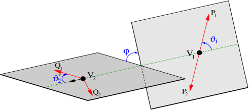
Figure 6.1: Definition of the various angles in the decay $B\to V_{1}(\to P_{1}P_{2})V_{2}(\to Q_{1}Q_{2})$.

There are different ways to perform the angular integrations in order to extract the purely longitudinal component from the differential decay rate. A first option consists in computing moments of $\cos\theta_{1}$ (or equivalently $\cos\theta_{2}$) :

$$\Gamma^{\rm long}\equiv\int\frac{d^{3}\Gamma}{d\cos\theta_{1}d\cos\theta_{2}d\phi}\left(\frac{5}{2}\cos^{2}\theta_{1}-\frac{1}{2}\right)d\cos\theta_{1}d\cos\theta_{2}d\phi=g_{PS}|A_{0}|^{2}/\tau_{B}$$ (6.4)

where $g_{PS}$ is the product of phase-space and lifetime factors

$$g_{PS}=\frac{\tau_{B}}{16\pi M_{B}^{3}}\sqrt{[M_{B}^{2}-(m_{1}+m_{2})^{2}][M_{B}^{2}-(m_{1}-m_{2})^{2}]}$$ (6.5)

A second possibility amounts to performing asymmetric integrations over one angle [135]

$$\Gamma^{\rm long}\equiv\int_{-1}^{1}d\cos\theta_{1}\int_{T}d\cos\theta_{2}\int_{0}^{2\pi}d\phi\frac{d^{3}\Gamma}{d\cos\theta_{1}d\cos\theta_{2}d\phi}=g_{PS}|A_{0}|^{2}/\tau_{B}$$ (6.6)

with

$$\int_{T}d\cos\theta_{2}=\left(\frac{11}{9}\int_{0}^{\pi/3}-\frac{5}{9}\int_{\pi/3}^{2\pi/3}+\frac{11}{9}\int_{2\pi/3}^{\pi}\right)(-\sin\theta_{2})d\theta_{2}$$ (6.7)

In the same way we can obtain the CP-conjugate $\Gamma^{\rm long}({\bar{B}_{q}^{0}}\to\bar{f})$ from the corresponding CP-conjugate distribution, leading to the CP-averaged branching ratio of the longitudinal component

$$BR^{\rm long}=\frac{\tau_{B}}{2}\left({\Gamma^{\rm long}(B^{0}_{q}\to f)+\Gamma^{\rm long}(\bar{B}^{0}_{q}\to\bar{f})}\right)=g_{PS}\frac{|A_{0}|^{2}+|\bar{A}_{0}|^{2}}{2}$$ (6.8)

where $\bar{A}_{0}$ is the CP-conjugate amplitude of $A_{0}$.

If we include the dependence on time in the above expressions, $B$-$\bar{B}$ mixing modifies the expressions. We will focus on CP-eigenstates $f_{\rm\scriptscriptstyle CP}$ in the final state $K^{*0}\bar{K}^{*0}$ and $\phi\phi$, as well as $\phi K^{*0}$ with a subsequent decay of $K^{*0}$ into a CP-eigenstate ($K_{s}\pi^{0}$ or $K_{L}\pi^{0}$).

The time evolution of these observables is obtained by considering the time dependence of $A_{0}(t)$ [136]. Inserting this time dependence one arrives at the usual expression for the longitudinal component of the time-dependent CP-asymmetry:

$$\mathcal{A}^{\rm long}_{\rm CP}(t)\equiv\frac{\Gamma^{\rm long}(B^{0}_{q}(t)\to f_{\rm\scriptscriptstyle CP})-\Gamma^{\rm long}(\bar{B}^{0}_{q}(t)\to f_{\rm\scriptscriptstyle CP})}{\Gamma^{\rm long}(B^{0}_{q}(t)\to f_{\rm\scriptscriptstyle CP})+\Gamma^{\rm long}(\bar{B}^{0}_{q}(t)\to f_{\rm\scriptscriptstyle CP})}=\frac{\mathcal{A}_{\rm dir}^{\rm long}\cos{(\Delta Mt)}+\mathcal{A}_{\rm mix}^{\rm long}\sin{(\Delta Mt)}}{\cosh{(\Delta\Gamma t/2)}-\mathcal{A}^{\rm long}_{\Delta\Gamma}\sinh{(\Delta\Gamma t/2)}}$$ (6.9)

where the direct and mixing-induced CP asymmetries are defined by:

$$\mathcal{A}_{\rm dir}^{\rm long}\equiv\frac{|A_{0}|^{2}-|\bar{A}_{0}|^{2}}{|A_{0}|^{2}+|\bar{A}_{0}|^{2}},\quad\mathcal{A}_{\rm mix}^{\rm long}\equiv-2\frac{{\rm Im}(e^{-i\phi_{M}}A_{0}^{*}\bar{A_{0}})}{|A_{0}|^{2}+|\bar{A_{0}}|^{2}}$$ (6.10)

together with the asymmetry related to the width difference :

$$\mathcal{A}^{\rm long}_{\Delta\Gamma}\equiv-2\frac{{\rm Re}(e^{-i\phi_{M}}A_{0}^{*}\bar{A_{0}})}{|A_{0}|^{2}+|\bar{A_{0}}|^{2}}$$ (6.11)

$\phi_{M}$ is the mixing angle and $\Delta\Gamma=\Gamma^{H}-\Gamma^{L}$. $\eta_{f}$ is the CP eigenvalue of the final state $f$ ($\pm 1$): $\eta_{K^{*0}K^{*0}}=\eta_{\phi\phi}=1$, whereas $\eta_{K^{*0}\phi}=1$ if $K^{*0}$ decays into $K_{s}\pi^{0}$ and $-1$ if it decays into $K_{L}\pi^{0}$. In the latter case, the contribution from the strong process $K^{*0}\to K\pi$ is the same for both $B$ and $\bar{B}$ decays and it cancels in the time-dependent CP-asymmetry Eq.(6.10), which depends only on the amplitudes $A_{0}$ and $\bar{A}_{0}$.

Finally, if the direct CP-asymmetries of all three helicity components are negligible, the longitudinal branching ratio can be estimated very easily from: $BR^{\rm long}=BR^{\rm total}f_{0}$.

6.2 Inputs

In this section we compute the values of the quantities $\Delta$ for the decays $B_{d,s}\to K^{*0}\bar{K}^{*0}$, $B_{d,s}\to\phi K^{*0}$ and $B_{s}\to\phi\phi$. Because the final states can appear in three different polarization states, a different $\Delta$ should be associated to each polarization. However, since we are only interested in longitudinal polarizations, we only give the results for this case.

For $B_{d,s}\to K^{*0}\bar{K}^{*0}$ we obtain,

$$|\Delta^{d}_{\scriptscriptstyle K^{*}K^{*}}| = A_{\scriptscriptstyle K^{*}K^{*}}^{d,0}\frac{C_{F}\alpha_{s}}{4\pi N_{c}}C_{1}\,|\bar{G}_{\scriptscriptstyle K^{*}}(s_{c})-\bar{G}_{\scriptscriptstyle K^{*}}(0)|=(1.85\pm 0.79)\times 10^{-7}\ {\rm GeV}\qquad$$ (6.12)

$$|\Delta^{s}_{\scriptscriptstyle K^{*}K^{*}}| = A_{\scriptscriptstyle K^{*}K^{*}}^{s,0}\frac{C_{F}\alpha_{s}}{4\pi N_{c}}C_{1}\,|\bar{G}_{\scriptscriptstyle K^{*}}(s_{c})-\bar{G}_{\scriptscriptstyle K^{*}}(0)|=(1.62\pm 0.69)\times 10^{-7}\ {\rm GeV}\qquad$$ (6.13)

where $\bar{G}_{V}\equiv G_{V}-r_{\chi}^{V}\hat{G}_{V}$ are the usual penguin functions and $A_{V_{1}V_{2}}^{q,0}$ are the naive factorization factors combining decay constants and form factors (see Sections 2.1.2 and 5.1). The numerical values of the used inputs are given in Table 6.1, which are taken from Ref. [28]. The contributions to each error from the various sources are detailed in Table 6.2.

The conditions in eqs. (5.10) derived in Chapter 5 can be applied to the $B_{d}\to K^{*0}\bar{K}^{*0}$ longitudinal branching ratio and CP asymmetry given the value for $\Delta^{d}_{\scriptscriptstyle K^{*}K^{*}}$ in eq. (6.12). The allowed region in the observable space is shown in Fig. 6.2.

\psfrag{BR}{$BR^{\rm long}(B_{d}\to K^{*0}\bar{K}^{*0})\times 10^{6}$}\psfrag{A}{$\mathcal{A}_{\rm dir}^{\rm long}(B_{d}\to K^{*0}\bar{K}^{*0})$}\psfrag{-0.4}{\hskip 4.26773pt$-0.4$}\psfrag{-0.2}{\hskip 4.26773pt$-0.2$}\psfrag{0.2}{\hskip 4.26773pt$0.2$}\psfrag{0.4}{\hskip 4.26773pt$0.4$}\psfrag{0}{$0$}\psfrag{2}{$2$}\psfrag{4}{$4$}\psfrag{6}{$6$}\psfrag{8}{$8$}\includegraphics[width=284.52756pt]{BRvsAdirKK.eps}

Figure 6.2: Allowed region on the $BR^{\rm long}-\mathcal{A}_{\rm dir}^{\rm long}$ plane for $B_{d}\to K^{*0}\bar{K}^{*0}$, according to the value of $\Delta^{d}_{\scriptscriptstyle K^{*}K^{*}}$.

For the $\Delta$, as well as for the other quantities computed in this chapter (as well as in Chapter 5), we quote as the central value the value obtained from taking the central value of the inputs. To estimate the error, we vary one by one each of the inputs, compute the difference with the central value, then add in quadrature the resulting uncertainties. The main sources of uncertainties are the scale of factorization $\mu$, the mass of the charm quark $m_{c}$, and the form factor $A_{0}^{B\to K*}$.

$m_{c}(m_{b})$	$f_{B}$	$f_{B_{s}}$	$\lambda_{B},\lambda_{B_{s}}$	$\alpha_{1}^{\bot}(K^{*})$
$\ 1.3\pm 0.2\$	$\ 0.21\pm 0.02\$	$\ 0.24\pm 0.02\$	$\ 0.35\pm 0.15\$	$\ 0.06\pm 0.06\$

$\alpha_{2}^{\bot}(K^{*})$	$f_{K^{*}}$	$f_{K^{*}}^{\bot}(2{\rm GeV})$	$A_{0}^{B\to K^{*}}$	$A_{0}^{B_{s}\to K^{*}}$
$\ 0.1\pm 0.2\$	$\ 0.218\pm 0.004\$	$\ 0.175\pm 0.025\$	$\ 0.39\pm 0.06\$	$\ 0.33\pm 0.05\$

$f_{\phi}$	$f_{\phi}^{\bot}(2{\rm GeV})$	$A_{0}^{B_{s}\to\phi}$	$\alpha_{2}^{\bot}(\phi)$
$\ 0.221\pm 0.003\$	$\ 0.175\pm 0.025\$	$\ 0.38^{+0.10}_{-0.02}\$	$\ 0.0\pm 0.3\$

Table 6.1: Input parameters required in QCD factorisation to compute the quantities $\Delta$’s and $\delta$’s described in the text. The masses and decay constants are given in GeV.

	$m_{c}$	$A_{0}^{B\to K^{*}}$	$f_{K^{*}}$	$\mu$	$\alpha_{1}(K^{*})$	$\alpha_{2}(K^{*})$	$\alpha_{1}^{\bot}(K^{*})$	$\alpha_{2}^{\bot}(K^{*})$
$\Delta^{d}_{K^{*}K^{*}}$	37.3%	13.2%	0.2%	44.2%	0.1%	4.6%	0.1%	0.3%
$\Delta^{s}_{K^{*}K^{*}}$	37.5%	12.9%	0.2%	44.4%	0.1%	4.7%	0.1%	0.3%

	$m_{c}$	$A_{0}^{B\to K^{*}}$	$f_{K^{*}}$	$f_{K^{*}}^{\bot}(2{\rm GeV})$	$\mu$	$\alpha_{1}(K^{*})$
$\Delta^{d}_{\phi K^{*}}$	44.2%	2.0%	—	—	52.3%	—
$\Delta^{s}_{\phi K^{*}}$	35.0%	—	0.1%	0.7%	58.2%	0.7%
$\Delta^{s}_{\phi\phi}$	44.1%	—	—	—	52.3%	—

	$\alpha_{2}(K^{*})$	$\alpha_{2}^{\bot}(K^{*})$	$A_{0}^{B\to\phi}$	$f_{\phi}^{\bot}(2{\rm GeV})$	$\alpha_{2}(\phi)$	$\alpha_{2}^{\bot}(\phi)$
$\Delta^{d}_{\phi K^{*}}$	—	—	—	0.4%	0.7%	0.3%
$\Delta^{s}_{\phi K^{*}}$	0.1%	0.1%	5.0%	0%	0%	0%
$\Delta^{s}_{\phi\phi}$	—	—	2.1%	0.4%	0.7%	0.3%

Table 6.2: Relative contributions from the inputs to the errors in $\Delta$ for the various decays.

In a similar way, we can compute the corresponding longitudinal $\Delta$ for the decay modes $B_{d,s}\to\phi\bar{K}^{*0}$ and $B_{s}\to\phi\phi$:

$$|\Delta^{d}_{\phi K^{*}}| = A_{K^{*}\phi}^{d,0}\frac{C_{F}\alpha_{s}}{4\pi N_{c}}C_{1}\,|\bar{G}_{\phi}(s_{c})-\bar{G}_{\phi}(0)|=(1.02\pm 1.11)\times 10^{-7}\ {\rm GeV}\quad$$ (6.14)

$$|\Delta^{s}_{\phi K^{*}}| = A_{\phi K^{*}}^{s,0}\frac{C_{F}\alpha_{s}}{4\pi N_{c}}C_{1}\,|\bar{G}_{\phi}(s_{c})-\bar{G}_{\phi}(0)|=(1.16\pm 1.05)\times 10^{-7}\ {\rm GeV}\quad$$ (6.15)

$$|\Delta^{s}_{\phi\phi}| = A_{\phi\phi}^{s,0}\frac{C_{F}\alpha_{s}}{4\pi N_{c}}C_{1}\,|\bar{G}_{\phi}(s_{c})-\bar{G}_{\phi}(0)|=(2.06\pm 2.24)\times 10^{-7}\ {\rm GeV}\quad$$ (6.16)

In the following Sections we show how to apply the results of this section and Chapter 5 to the longitudinal contribution of penguin-dominated $B\to VV$ modes. We will see that they can be used to extract the $B_{s}-\bar{B_{s}}$ mixing angle and some longitudinal observables like branching ratios and time-dependent CP asymmetries within the Standard Model. In particular, we outline three different strategies to determine the $B_{s}-\bar{B_{s}}$ mixing angle (in the SM and beyond). Indeed, concerning New Physics we will see that under the assumption of no significant New Physics affecting the amplitude, while Strategy II can detect the presence of New Physics by comparing the obtained $\phi_{s}$ with $\phi_{s}^{SM}=2\beta_{s}$, Strategy I and III can not only detect New Physics but allow also for the extraction of $\phi_{s}$ even in the presence of New Physics in the mixing.

6.3 First strategy to extract $\phi_{s}$: Bounding $T/P$

The $b\to s$ penguin-dominated decays like $B_{s}\to K^{*0}\bar{K}^{*0}$ are in principle clean modes to extract the mixing angle $\phi_{s}$. In this section and those following, $\phi_{s}$ refers to the same mixing angle that will be measured, for instance, in the mixing induced CP asymmetry of $B_{s}\to\psi\phi$ including possible New Physics contributions in the mixing. When focusing only on SM we will use the notation $\phi_{s}=2\beta_{s}$.

In an expansion in powers of $\lambda_{u}^{(s)}/\lambda_{c}^{(s)}$, the amplitude for the decay $B_{s}\to K^{*0}\bar{K}^{*0}$ is given by:

$$\mathcal{A}_{\rm mix}^{\rm long}(B_{s}\to K^{*0}\bar{K}^{*0})\simeq\sin{\phi_{s}}+2\left|\frac{\lambda_{u}^{(s)}}{\lambda_{c}^{(s)}}\right|{\rm Re}\left(\frac{T^{s}_{K^{*}K^{*}}}{P^{s}_{K^{*}K^{*}}}\right)\sin{\gamma}\cos{\phi_{s}}+\cdots$$ (6.17)

In order to determine the accuracy of this relation, we must assess the size of the CKM-suppressed hadronic contribution $T$. Notice that this relation is valid even in presence of New Physics in the mixing. In the SM, one can derive from the Wolfenstein parametrisation that eq. (6.17) is of order $\lambda^{2}$ (with $\lambda=V_{us}$), and both pieces shown on the r.h.s of eq.(6.17) are of this same order. However, despite the smallness of the ratio $|\lambda_{u}^{(s)}/\lambda_{c}^{(s)}|=0.044$, a significant value of the hadronic ratio ${\rm Re}(T/P)$ could spoil the potentially safe extraction of $\sin{\phi_{s}}$. The deviation from $\sin\phi_{s}$ is:

$$\Delta S(B_{s}\to K^{*0}\bar{K}^{*0})\equiv 2\left|\frac{\lambda_{u}^{(s)}}{\lambda_{c}^{(s)}}\right|{\rm Re}\left(\frac{T^{s}_{K^{*}K^{*}}}{P^{s}_{K^{*}K^{*}}}\right)\sin{\gamma}\cos{\phi_{s}}$$ (6.18)

We want to set bounds on ${\rm Re}(T/P)$, which can be related to the inputs:

$${\rm Re}\left(\frac{T}{P}\right)={\rm Re}\left(\frac{P+\Delta}{P}\right)=1+{\rm Re}\left(\frac{\Delta}{P}\right)=1+\frac{{\rm Re}(P)\,\Delta}{{\rm Re}(P)^{2}+{\rm Im}(P)^{2}}$$ (6.19)

Eqs. (5.11) show that the maximum of ${\rm Re}(T/P)$ is reached for $\mathcal{A}_{\rm dir}^{\rm long}=0$ together with the positive branch for ${\rm Re}(P)$. The following bound is obtained

$${\rm Re}\left(\frac{T}{P}\right)\leq\,1+\left(-c_{1}^{(s)}+\sqrt{-(c_{0}^{(s)}/c_{2}^{(s)})^{2}+(1/c_{2}^{(s)})\,\widetilde{BR}/\Delta^{2}}\right)^{-1}$$ (6.20)

where the lower bound for $BR^{\rm long}$ and the upper bound for $\Delta$ must be used. In a similar way, the minimum of ${\rm Re}(T/P)$ occurs for $\mathcal{A}_{dir}^{\rm long}=0$, for the negative branch of Eq. (5.11) for the solution of ${\rm Re}(P)$

$${\rm Re}\left(\frac{T}{P}\right)\geq\,1+\left(-c_{1}^{(s)}-\sqrt{-(c_{0}^{(s)}/c_{2}^{(s)})^{2}+(1/c_{2}^{(s)})\,\widetilde{BR}/\Delta^{2}}\right)^{-1}$$ (6.21)

where the lower bound for $BR^{\rm long}$ and the upper bound for $\Delta$ must be used once again. As a conclusion, we obtain a range for ${\rm Re}(T/P)$ from two inputs: the branching ratio $BR^{\rm long}(B_{s}\to K^{*0}\bar{K}^{*0})$ and $\Delta^{s}_{K^{*}K^{*}}$, given in Eq.(6.13).

\psfrag{S}{\small$\Delta S(B_{s}\to K^{*0}\bar{K}^{*0})$}\psfrag{BR}{\small$BR^{\rm long}(B_{s}\to K^{*0}\bar{K}^{*0})\times 10^{6}$}\psfrag{10}{\small$10$}\psfrag{20}{\small$20$}\psfrag{30}{\small$30$}\psfrag{40}{\small$40$}\psfrag{50}{\small$50$}\psfrag{0.03}{\small$0.03$}\psfrag{0.035}{\small$0.035$}\psfrag{0.04}{\small$0.04$}\psfrag{0.045}{\small$0.045$}\psfrag{0.05}{\small$0.05$}\psfrag{0.055}{\small$0.055$}\psfrag{0.06}{\small$0.06$}\includegraphics[height=170.71652pt]{DeltaSBstoKK.eps}

Figure 6.3: Absolute bounds on $\Delta S(B_{s}\to K^{*0}\bar{K}^{*0})$ as a function of the longitudinal branching ratio $BR^{\rm long}(B_{s}\to K^{*0}\bar{K}^{*0})$.

Using Eq. (6.18), these upper and lower bounds on ${\rm Re}(T/P)$ are converted into a bound on the pollution $\Delta S(B_{s}\to K^{*0}\bar{K}^{*0})$. The latter is plotted as a function of the longitudinal $BR^{\rm long}(B_{s}\to K^{*0}\bar{K}^{*0})$ in Fig.6.3.

Once a measurement of $\mathcal{A}_{\rm mix}^{\rm long}(B_{s}\to K^{*0}\bar{K}^{*0})$ is available, upper and lower bounds for $\phi_{s}$ are easily obtained. For instance, if we take as a lower bound for the branching ratio $BR^{\rm long}(B_{s}\to K^{*0}\bar{K}^{*0})\gtrsim 5\times 10^{-6}$, Fig. 6.3 gives $0.03<\Delta S(B_{s}\to K^{*0}\bar{K}^{*0})<0.06$. In the case of a moderately large branching ratio $BR^{\rm long}(B_{s}\to K^{*0}\bar{K}^{*0})\sim(30-40)\,\times 10^{-6}$, the bounds get sharper, with $0.04<\Delta S(B_{s}\to K^{*0}\bar{K}^{*0})<0.05$ and

$$\big{(}\mathcal{A}_{\rm mix}^{\rm long}(B_{s}\to K^{*0}\bar{K}^{*0})-0.05\big{)}\ <\sin{\phi_{s}}<\ \big{(}\mathcal{A}_{\rm mix}^{\rm long}(B_{s}\to K^{*0}\bar{K}^{*0})-0.04\big{)}$$ (6.22)

The same strategy can be applied to $B_{s}\to\phi K^{*0}$ and $B_{s}\to\phi\phi$ decays

• Take the experimental value for the longitudinal branching ratio $BR^{\rm long}$ (once available), and the theoretical value for $\Delta$ from Eqs. (6.15) or (6.16).

• Apply Eqs. (6.20) and (6.21) to constrain the range of ${\rm Re}(T/P)$.

• Derive the allowed range for $\Delta S$ according to the equivalent of (6.18)

• From the measured value of $\mathcal{A}_{\rm mix}^{\rm long}$, determine $\phi_{s}$ from

  $$\big{(}\mathcal{A}_{\rm mix}^{\rm long}-\Delta S_{max}\big{)}\ <\sin{\phi_{s}}<\ \big{(}\mathcal{A}_{\rm mix}^{\rm long}-\Delta S_{min}\big{)}$$ (6.23)

A weak mixing angle $\phi_{s}$ different from $\phi_{s}^{SM}$ would signal the presence of New Physics.

Interestingly, if the longitudinal direct CP asymmetry becomes available and happens to be inconsistent with zero, the bounds for ${\rm Re}(T/P)$ in Eq. (6.20) and (6.21) can be tightened. Eq. (6.19) can be exploited to derive expressions similar to Eq. (6.20) and (6.21) with a non-vanishing $\mathcal{A}_{\rm dir}^{\rm long}$, leading to stronger bounds on ${\rm Re}(T/P)$ and consequently on $\sin\phi_{s}$.

6.4 Second strategy : Measuring CP asymmetries and BR

In this section, we show how we can extract mixing angles and related CKM phases in a clean way from experimental data, the length of two sides of the unitarity triangle and the theoretical quantity $\Delta$. The only theoretical requirement is that the decay must allow for a safe way of computing $\Delta$. The approach is general in the same sense as in the previous section, since it can be applied to any B decay into two pseudoscalars or vectors. But it yields different results for the four groups of decays:

1. $B_{d}$ decay through a $b\to d$ process, e.g. $B_{d}\to K^{*0}\bar{K}^{*0}$

2. $B_{s}$ decay through a $b\to s$ process, e.g. $B_{s}\to K^{*0}\bar{K}^{*0}$

3. $B_{d}$ decay through a $b\to s$ process, e.g. $B_{d}\to\phi\bar{K}^{*0}$ (with a subsequent decay into a CP eigenstate)

4. $B_{s}$ decay through a $b\to d$ process, e.g. $B_{s}\to\phi\bar{K}^{*0}$ (with a subsequent decay into a CP eigenstate)

As far as weak interactions are concerned, the difference between $B_{d}$ and $B_{s}$ decays consists in the mixing angle, whereas $b\to d$ and $b\to s$ processes differ through the CKM elements $\lambda_{u,c}^{(D)}$, where $D=d$ or $s$.

In the case of a $B_{d}$ meson decaying through a $b\to D$ process $(D=d,s)$, we can extract the angles $\alpha$ [38] and $\beta$ from the identities:

$$\sin^{2}{\alpha} = \frac{\widetilde{BR}}{2|\lambda_{u}^{(D)}|^{2}|\Delta|^{2}}\left(1-\sqrt{1-{(\mathcal{A}_{\rm dir})}^{2}-{(\mathcal{A}_{\rm mix})}^{2}}\right)$$ (6.24)

$$\sin^{2}{\beta} = \frac{\widetilde{BR}}{2|\lambda_{c}^{(D)}|^{2}|\Delta|^{2}}\left(1-\sqrt{1-{(\mathcal{A}_{\rm dir})}^{2}-{(\mathcal{A}_{\rm mix})}^{2}}\right)$$ (6.25)

In the case of a $B_{s}$ meson decaying through a $b\to D$ process $(D=d,s)$, we can extract the angles $\beta_{s}$ [137] and $\gamma$, assuming no New Physics in the decay, from the following expressions:

$$\sin^{2}{\beta_{s}} = \frac{\widetilde{BR}}{2|\lambda_{c}^{(D)}|^{2}|\Delta|^{2}}\left(1-\sqrt{1-{(\mathcal{A}_{\rm dir})}^{2}-{(\mathcal{A}_{\rm mix})}^{2}}\right)$$ (6.26)

$$\sin^{2}{\left(\beta_{s}+\gamma\right)} = \frac{\widetilde{BR}}{2|\lambda_{u}^{(D)}|^{2}|\Delta|^{2}}\left(1-\sqrt{1-{(\mathcal{A}_{\rm dir})}^{2}-{(\mathcal{A}_{\rm mix})}^{2}}\right)$$ (6.27)

If the obtained $\beta_{s}$ differs from its SM value, this would signal the presence of New Physics. Notice that this strategy is obtained by combining the definition of $\Delta$ with the unitarity of the CKM matrix, so it is designed to work only in the context of the SM. Consequently the previous expressions should be understood as a way of testing the SM. This is an important difference with Strategies I and III where one can obtain a value for the weak mixing phase also in the presence of New Physics in the mixing (but not in the decay).

While the previous equations are quite general (they can be used for $B\to PP$ decays), it is understood that $BR$ and $A_{\rm dir,mix}$ refer to the longitudinal branching ratio and longitudinal CP-asymmetries, respectively, when they are applied to $B\to VV$ decays.

Eq. (6.26) provides a new way to perform a consistency test for the SM value of $|\sin\beta_{s}|$ from the measurements of $\mathcal{A}_{\rm mix}^{\rm long}(B_{s}\to K^{*0}\bar{K}^{*0})$, $\mathcal{A}_{\rm dir}^{\rm long}(B_{s}\to K^{*0}\bar{K}^{*0})$ and $BR^{\rm long}(B_{s}\to K^{*0}\bar{K}^{*0})$. The same strategy can be applied to $B_{s}\to\phi\bar{K}^{*0}$ and $B_{s}\to\phi\phi$ using the corresponding sum rules. This sum rule offers several advantages : it is independent of CKM angles, and all the hadronic input is concentrated on a single well-controlled quantity $\Delta$.

Note that all these equations depend actually on the corresponding branching ratio and $\mathcal{A}_{\Delta\Gamma}^{\rm long}$. The asymmetry $\mathcal{A}_{\Delta\Gamma}^{\rm long}$ is indeed related to the direct and mixing-induced CP-asymmetries through the equality ${(\mathcal{A}_{\rm dir}^{\rm long})}^{2}+{(\mathcal{A}_{\rm mix}^{\rm long})}^{2}+{(\mathcal{A}_{\Delta\Gamma}^{\rm long})}^{2}=1$. It was already noticed in [128] in the context of $B_{s}\to K^{+}K^{-}$ and in [138] in the context of $B\to J/\psi K^{*},D^{\ast+}_{s}\bar{D}^{\ast}$ decays that it is possible to extract $\mathcal{A}_{\Delta\Gamma}^{\rm long}$ directly from the “untagged” rate:

$$\Gamma^{\rm long}(B_{s}(t)\to VV)+\Gamma^{\rm long}(\overline{B_{s}}(t)\to VV)\propto R_{\rm H}e^{-\Gamma_{\rm H}^{(s)}t}+R_{\rm L}e^{-\Gamma_{\rm L}^{(s)}t}$$ (6.28)

If the time dependence of both exponentials can be separated, one obtains

$$\mathcal{A}_{\Delta\Gamma}^{\rm long}(B_{s}\to VV)=\frac{R_{\rm H}-R_{\rm L}}{R_{\rm H}+R_{\rm L}},$$ (6.29)

The branching ratio and $\mathcal{A}_{\Delta\Gamma}^{\rm long}$ are thus the only required observables to extract $\beta_{s}$ through this method, which offers the advantage of concentrating in $\Delta$ all the hadronic input needed to bound the tree-to-penguin ratio.

6.5 Third strategy : Relating $B_{s}\to K^{*0}\bar{K}^{*0}$ and $B_{d}\to K^{*0}\bar{K}^{*0}$

Once an angular analysis of $B_{d}\to K^{*0}\bar{K}^{*0}$ is performed, it is possible to extract the CP-averaged branching ratio corresponding to the longitudinal helicity final state. Eqs. (5.11) can be used to extract the hadronic parameters, if one assumes that no New Physics contributes in an appreciable way. If flavor symmetries are sufficiently accurate for this particular process, this estimate can be converted into a fairly precise determination of hadronic parameters for the $b\to s$ channel $B_{s}\to K^{*0}\bar{K}^{*0}$. We have seen in Chapter 5 that for $B_{d,s}\to KK$ modes a $U$-spin analysis combined with QCD factorization leads to tight constraints on the ratio of the tree contributions to both decay modes, as well as that for the penguins. In this section we show how to relate $B_{d}\to K^{*0}\bar{K}^{*0}$ and $B_{s}\to K^{*0}\bar{K}^{*0}$ decay modes following the same approach.

\psfrag{ReP}{\small${\rm Re}(P_{\scriptscriptstyle K^{*}K^{*}}^{d})\ (\times 10^{-6})$}\psfrag{ImP}{\small${\rm Im}(P_{\scriptscriptstyle K^{*}K^{*}}^{d})\ (\times 10^{-6})$}\includegraphics[height=170.71652pt]{PBstoKK.eps}

Figure 6.4: Values for $P_{\scriptscriptstyle K^{*}K^{*}}^{d}$ corresponding to a real $\Delta_{K^{*}K^{*}}$, as a function of the longitudinal observables $BR^{0}(B_{d}\to K^{*0}\bar{K}^{*0})$ and $Adir^{0}(B_{d}\to K^{*0}\bar{K}^{*0})$. The contours from black to gray correspond to branching ratios from $10^{-6}$ to $10^{-5}$ in steps of $2.5\times 10^{-6}$. The contours from red to yellow correspond to values of the CP asymmetry from $0$ to its maximum allowed value in steps of 30% of its maximum value. The contours from red to pink are the same for negative CP asymmetry.

We define the parameters $\delta_{\scriptscriptstyle K^{*}K^{*}}^{P}$ and $\delta_{\scriptscriptstyle K^{*}K^{*}}^{T}$ as

$$\begin{array}[]{rclcrcl}P_{K^{*}K^{*}}^{s}&=&f\,P_{K^{*}K^{*}}^{d}(1+\delta_{\scriptscriptstyle K^{*}K^{*}}^{P})\ ,&&T_{K^{*}K^{*}}^{s}&=&f\,T_{K^{*}K^{*}}^{d}(1+\delta_{\scriptscriptstyle K^{*}K^{*}}^{T})\\ \end{array}$$ (6.30)

where the factor $f$ is given by

$$\frac{m_{B_{s}}^{2}A_{0}^{B_{s}\to K^{*}}}{m_{B}^{2}A_{0}^{B\to K^{*}}}=0.88\pm 0.19$$ (6.31)

We compute $|\delta_{\scriptscriptstyle K^{*}K^{*}}^{P,T}|$ using QCDF. These parameters are affected by the model dependent treatment of annihilation and spectator-scattering contributions, so the results should be considered as an estimate. A significant part of long-distance dynamics is common to both decays, and we find the following upper bounds

$$|\delta_{\scriptscriptstyle K^{*}K^{*}}^{P}|\leq 0.12\ ,\qquad|\delta_{\scriptscriptstyle K^{*}K^{*}}^{T}|\leq 0.15$$ (6.32)

where the largest contribution comes from the lower value of $\lambda_{B}$.

We could in principle apply the same strategy to $B_{d,s}\to\phi K^{*0}$, but the corresponding $\delta$’s are much larger. Indeed, the computation leads to corrections up to $\delta_{\scriptscriptstyle\phi K^{*}}\sim 50\%$. This shows that $U$-spin symmetry cannot be expected to hold at a high accuracy for any pair of flavour-related processes. $K^{(*)}K^{(*)}$ offer a much more interesting potential than other final states such as $\phi K^{*0}$. Moreover, we cannot perform a similar analysis for $\phi\phi$ since $B_{d}\to\phi\phi$ is a pure weak-annihilation process, contrary to $B_{s}\to\phi\phi$ mediated through penguins. Therefore we focus on the precise $B_{s}\to K^{*0}{\bar{K}^{*0}}$ modes in the remaining part of this section. Notice that the large hadronic uncertainties affecting $B_{s}\to\phi\phi$ and $B_{s}\to\phi K^{*0}$ have no impact when we use these modes in the strategies described in Sections 6.3 and 6.4, since we exploited a quantity $\Delta$ where they cancel out.

\psfrag{BRd}{$BR^{\rm long}(B_{d}\to K^{*0}\bar{K}^{*0})\times 10^{6}$}\psfrag{BRs}{$BR^{\rm long}(B_{s}\to K^{*0}\bar{K}^{*0})\times 10^{6}$}\includegraphics[height=170.71652pt]{BRBstoKK.eps}

Figure 6.5: Longitudinal branching ratio for $B_{s}\to K^{*0}\bar{K}^{*0}$ in terms of the longitudinal $B_{d}\to K^{*0}\bar{K}^{*0}$ branching ratio. The light-shaded area corresponds to the uncertainty on the ratio of form factors $f$, whereas the dark-shaded area comes from varying the various hadronic inputs.

Once the hadronic parameters $P_{K^{*}K^{*}}^{s}$ and $T_{K^{*}K^{*}}^{s}$ have been obtained from Eq.(6.30), one can give predictions for the $B_{s}\to K^{*0}\bar{K}^{*0}$ observables. Note that the branching ratio $BR^{\rm long}(B_{d}\to K^{*0}\bar{K}^{*0})$ is an experimental input in this analysis, and this piece of information is not available yet. The result for the branching ratio of $B_{s}\to K^{*0}\bar{K}^{*0}$ is given in terms of the $B_{d}\to K^{*0}\bar{K}^{*0}$ branching ratio in Fig.6.5. Once the branching ratio of $B_{d}\to K^{*0}\bar{K}^{*0}$ is measured one can use this plot to find the SM prediction for $BR^{\rm long}(B_{s}\to K^{*0}\bar{K}^{*0})$.

The ratio of branching ratios $BR^{\rm long}(B_{s}\to K^{*0}\bar{K}^{*0})/BR^{\rm long}(B_{d}\to K^{*0}\bar{K}^{*0})$ and the asymmetries turn out to be quite insensitive to the exact value of $BR^{\rm long}(B_{d}\to K^{*0}\bar{K}^{*0})$ as long as $BR^{\rm long}(B_{d}\to K^{*0}\bar{K}^{*0})\gtrsim 5\times 10^{-7}$. The numerical values are summarised in Table 6.3.

$\begin{array}[]{c}\\ \quad\displaystyle\left(\frac{BR^{\rm long}(B_{s}\to K^{*0}\bar{K}^{*0})}{BR^{\rm long}(B_{d}\to K^{*0}\bar{K}^{*0})}\right)_{\scriptscriptstyle SM}=17\pm 6\\ \\ \end{array}$
$\begin{array}[]{c}\\ \mathcal{A}_{\rm dir}^{\rm long}(B_{s}\to K^{*0}\bar{K}^{*0})_{\scriptscriptstyle SM}=0.000\pm 0.014\\ \\ \end{array}$
$\begin{array}[]{c}\\ \mathcal{A}_{\rm mix}^{\rm long}(B_{s}\to K^{*0}\bar{K}^{*0})_{\scriptscriptstyle SM}=0.004\pm 0.018\\ \\ \end{array}$

Table 6.3: Results for the longitudinal observables related to $B_{s}\to K^{*0}\bar{K}^{*0}$ according to Sec. 6.5. These are predictions for the SM contributions under the standard assumption of no New Physics in $b\to d$ transition. We used $\phi_{s}^{SM}=2\beta_{s}=-2^{\circ}$ for $\mathcal{A}_{\rm mix}^{\rm long}$, and we assumed $BR^{\rm long}(B_{d}\to K^{*0}\bar{K}^{*0})\gtrsim 5\times 10^{-7}$. The quoted uncertainty includes the errors associated to all input parameters including the variation of $\gamma$ inside the range $56^{\circ}\leq\gamma\ \leq 68^{\circ}$ [74, 75].

Under the standard assumption that New Physics contribution to $b\to d$ penguins is negligible, and since the experimental input comes entirely from $B_{d}\to K^{*0}\bar{K}^{*0}$ (a $b\to d$ penguin), the results given in Table 6.3 are SM predictions. In presence of New Physics in $b\to s$ penguins the full prediction can be obtained by adding to the SM piece extra contributions to the amplitude and weak mixing angle as explained in [126, 101, 139].

One may also use this as a strategy to extract the mixing angle $\phi_{s}$. If one assumes no New Physics in the decay $B_{s}\to K^{*0}\bar{K}^{*0}$, this method relates directly $\mathcal{A}_{\rm mix}^{\rm long}(B_{s}\to K^{*0}\bar{K}^{*0})$ and $\phi_{s}$. Fig.6.6 shows $\mathcal{A}_{\rm mix}^{\rm long}(B_{s}\to K^{*0}\bar{K}^{*0})$ vs. $\phi_{s}$. Once this asymmetry is measured, this plot can be used as a way to extract $\phi_{s}$, and this result can be compared to the one found in tree decays such as $B\to DK$. A disagreement would point out New Physics. Moreover, it is possible to distinguish whether New Physics affects the decay or the mixing itself, by confronting $BR^{\rm long}(B_{s}\to K^{*0}\bar{K}^{*0})$ and $\mathcal{A}_{\rm dir}^{\rm long}(B_{s}\to K^{*0}\bar{K}^{*0})$ with the SM predictions given in Table 6.3. If the predictions for the branching ratio and the direct CP asymmetry agree with experiment, but the $\phi_{s}$ extracted from $\mathcal{A}_{\rm mix}^{\rm long}(B_{s}\to K^{*0}\bar{K}^{*0})$ differs from $\phi_{s}^{SM}$, this will be a clear indication of New Physics in $B_{s}-\bar{B}_{s}$ mixing. An interesting comparison will be allowed between the value for $\phi_{s}$ obtained here and the measurement of $\phi_{s}$ from the mixing induced CP-asymmetry of $B_{s}\to DK$ decay [140, 141].

\psfrag{phis}{$\phi_{s}$ (Degree)}\psfrag{Amix}{$\mathcal{A}_{\rm mix}^{\rm long}(B_{s}\to K^{*0}\bar{K}^{*0})$}\includegraphics[height=170.71652pt]{Amixphis.eps}

Figure 6.6: Relation between $\mathcal{A}_{\rm mix}^{\rm long}(B_{s}\to K^{*0}\bar{K}^{*0})$ and the $B_{s}-\bar{B}_{s}$ mixing angle $\phi_{s}$. We assumed $BR^{\rm long}(B_{d}\to K^{*0}\bar{K}^{*0})\gtrsim 5\times 10^{-7}$ and $\gamma=62^{\circ}$. A measurement of this asymmetry leads to a prediction for $\phi_{s}$, which includes hadronic pollution and SU(3) breaking effects, according to Sec. 6.5.

6.6 Discussion

The increasing list of measured non-leptonic two-body $B_{d}$- and $B_{s}$-decays provides many tests of the CKM mechanism of CP violation in the Standard Model. Of particular interest is the determination of angles through time-dependent CP-asymmetries. For instance $\phi_{s}$, related to $B_{s}-\bar{B}_{s}$ mixing, should be constrained : it is tiny in the Standard Model, and can be measured through many penguin-dominated decays. However, for such determination to be valid, one must assess the size of the various hadronic quantities involved as precisely as possible.

	Strategy 1	Strategy 2	Strategy 3
Inputs	$\begin{array}[]{c}\\ BR^{\rm long}(B_{s}\to K^{*0}\bar{K}^{*0})\\ \mathcal{A}_{\rm mix}^{\rm long}(B_{s}\to K^{*0}\bar{K}^{*0})\\ \Delta^{s}_{K^{*}K^{*}},\ \gamma\\ \\ \end{array}$	$\begin{array}[]{c}BR^{\rm long}(B_{s}\to K^{*0}\bar{K}^{*0})\\ \mathcal{A}_{\rm dir}^{\rm long}(B_{s}\to K^{*0}\bar{K}^{*0})\\ \mathcal{A}_{\rm mix}^{\rm long}(B_{s}\to K^{*0}\bar{K}^{*0})\\ \Delta^{s}_{K^{*}K^{*}}\end{array}$	$\begin{array}[]{c}BR^{\rm long}(B_{d}\to K^{*0}\bar{K}^{*0})\\ \mathcal{A}_{\rm mix}^{\rm long}(B_{s}\to K^{*0}\bar{K}^{*0})\\ \Delta^{d}_{K^{*}K^{*}},\ \delta_{T},\ \delta_{P},\ \gamma\end{array}$
Outputs	$\phi_{s}$	$|\sin{\beta_{s}}|$, $\gamma$	$\begin{array}[]{c}\\ BR^{\rm long}(B_{s}\to K^{*0}\bar{K}^{*0})_{\scriptscriptstyle SM}\\ \mathcal{A}_{\rm dir}^{\rm long}(B_{s}\to K^{*0}\bar{K}^{*0})_{\scriptscriptstyle SM}\\ \phi_{s}\\ \\ \end{array}$
Advantages	Applies also to $B_{s}\to\phi K^{*0}$ and $B_{s}\to\phi\phi$	Applies also to $B_{s}\to\phi K^{*0}$ and $B_{s}\to\phi\phi$	It can be easily generalized to include New Physics in the decay and mixing.
Limitations	It assumes no New Physics in $b\to s$ decay.	It assumes no New Physics in $b\to s$ decay.	Does not apply to $B_{s}\to\phi K^{*0}$ or $B_{s}\to\phi\phi$ because $\delta_{T,P}$ are big.

Table 6.4: Comparison between the three strategies for $B_{s}\to K^{*0}\bar{K}^{*0}$.

In this chapter we have applied ideas presented in Chapter 5 for $B_{d,s}\to KK$ to vector-vector modes mediated through penguins : $B_{d,s}\to K^{*0}\bar{K}^{*0}$, $\phi\phi$ and $\phi K^{*0}$ (with the condition that $K^{*0}$ decays into a definite-CP eigenstate). In order to combine flavor symmetries with QCD factorization, we have restricted our analysis to longitudinal observables, which are under better theoretical control. These observables have been related to the angular analysis performed experimentally in Sec. 6.1. Penguin-mediated modes offer the very interesting feature that the difference between tree and penguin contributions $\Delta=T-P$ should be dominated by short-distance physics. It can be computed fairly accurately using QCD factorization, and it can be used to determine tree and penguin contributions from observables as explained in Chapter 5. This theoretical piece of information is used to relate CP-asymmetries of $B_{d,s}\to K^{*0}\bar{K}^{*0}$, $\phi\phi$ and $\phi K^{*0}$ to CKM angles according to different strategies. For illustration, we have focused on $B_{d,s}\to K^{*0}\bar{K}^{*0}$, where all three strategies apply.

In Sec. 6.3, we have proposed to use $\Delta=T-P$ to put stringent bounds on the pollution due to hadronic uncertainties. Indeed, even though the ratio $|\lambda_{u}^{(s)}/\lambda_{c}^{(s)}|=0.044$ is small, a large value of the hadronic quantity ${\rm Re}(T/P)$ could spoil the naively safe extraction of $\sin{\phi_{s}}$ from the mixed asymmetry of $B_{s}\to K^{*0}\bar{K}^{*0}$. This strategy to control the pollution can be applied to all penguin-mediated processes of interest here. A similar analysis for $\sin{2\beta}$ from $B_{d}\to\phi K_{S}$ can be found in [40].

In Sec. 6.4, we have suggested a second approach, using $\mathcal{A}_{\rm mix}^{\rm long}(B_{s}\to K^{*0}\bar{K}^{*0})$, $\mathcal{A}_{\rm dir}^{\rm long}(B_{s}\to K^{*0}\bar{K}^{*0})$ and $BR^{\rm long}(B_{s}\to K^{*0}\bar{K}^{*0})$ to extract $|{\rm sin}\beta_{s}|$. In principle, one can also use an alternative set of experimental quantities : the branching ratio together with a direct measurement of the longitudinal untagged rate. The sum rule needed for the $B_{s}\to K^{*0}\bar{K}^{*0}$ is independent of the CKM angle $\gamma$ and the input on hadronic dynamics is limited to a single well-controlled quantity: $\Delta^{s}_{K^{*}K^{*}}$. This strategy can also be applied to extract $\beta_{s}$ from $B_{s}\to\phi\bar{K}^{*0}$ and $B_{s}\to\phi\phi$ using the corresponding sum rule.

In Sec. 6.5, we proposed a last method to determine $\phi_{s}$, by relying on the prediction of the mixing induced CP-asymmetry $\mathcal{A}_{\rm mix}^{\rm long}(B_{s}\to K^{*0}\bar{K}^{*0})$ as a function of the $BR^{\rm long}(B_{d}\to K^{*0}\bar{K}^{*0})$ and the theoretical input $\Delta^{d}_{K^{*}K^{*}}$. In this strategy, tree pollution is controlled using the hadronic information from flavour symmetry and QCD factorisation. The outcome of our analysis is presented in Fig. 6.6. This strategy requires data on $B_{d}\to K^{*0}\bar{K}^{*0}$ and on the mixing-induced CP-asymmetry $\mathcal{A}_{\rm mix}^{\rm long}(B_{s}\to K^{*0}\bar{K}^{*0})$. The input from $B_{s}$ decay is therefore minimal : $\mathcal{A}_{\rm mix}^{\rm long}(B_{s}\to K^{*0}\bar{K}^{*0})$, while all other inputs can be obtained from $B$-factories.

A comparison among the three different strategies discussed in this chapter is given in Table 6.4, where the needed inputs are enumerated as well as the predicted observables and the range of validity.

If both hadronic machines and super-$B$ factories [142] running at $\Upsilon(5S)$ provide enough information on $B_{s}$-decays, it will be interesting to compare the determination from $\phi_{s}$ following those methods, which rely on penguin-mediated decays, with the value obtained from tree processes like $B_{s}\to DK$. Differences between the values obtained through these two procedures would provide a clear hint of physics beyond the Standard Model. In such a situation, the different methods presented in this letter would yield very useful cross-checks for the penguin-dominated vector modes.

Chapter 7 Supersymmetric Contributions to $B_{s}^{\scriptscriptstyle 0}\to K^{+}K^{-}$ and $B_{s}^{\scriptscriptstyle 0}\to K^{\scriptscriptstyle 0}\bar{K}^{\scriptscriptstyle 0}$

In Section 4.5 we saw that the NP parameters for the decay $B_{s}^{\scriptscriptstyle 0}\to K^{+}K^{-}$ can be extracted from the measured values for the branching ratio and the CP-asymmetries, once the SM hadronic parameters are known. These hadronic parameters can be obtained from other decays related by flavor symmetries to $B_{s}^{\scriptscriptstyle 0}\to K^{+}K^{-}$, such as $B_{d}^{\scriptscriptstyle 0}\to\pi^{+}\pi^{-}$ or $B_{d}^{\scriptscriptstyle 0}\to K^{0}\bar{K}^{0}$, provided that these are not affected by NP. In Chapter 4 we obtained the $B_{s}^{\scriptscriptstyle 0}\to K^{+}K^{-}$ SM hadronic parameters from $B_{d}^{\scriptscriptstyle 0}\to\pi^{+}\pi^{-}$ using flavor symmetry, and in Chapter 5 we obtained the SM hadronic parameters of $B_{s}^{\scriptscriptstyle 0}\to K^{+}K^{-}$ and $B_{s}^{\scriptscriptstyle 0}\to K^{0}\bar{K}^{0}$ from $B_{d}^{\scriptscriptstyle 0}\to K^{0}\bar{K}^{0}$ using an interesting combination of flavor symmetry and QCDF.

Experimental values for the CP-asymmetries in $B_{s}^{\scriptscriptstyle 0}\to K^{+}K^{-}$ are still not available, so the method of Chapter 4 cannot be applied yet to measure the NP parameters $\mathcal{A}^{u}$ and $\Phi_{u}$. However, it is always interesting to study which existing NP models can generate sizeable contributions to these parameters, since once $\mathcal{A}^{u}$ and $\Phi_{u}$ are measured, these NP models will be the most sensitive to this new data. If they generate too big NP parameters, their parameter space will be drastically constrained. If the NP parameters are indeed measured to be large, then these models will prevail over more conservative ones.

On the other hand, being able to introduce hadronic effects in a fairly reliable way allows to give full predictions for observables in the presence of NP. Of course, no extension of the SM will be given full support until the SM predictions (and in particular those predictions derived in Chapters 4 and 5) are found inconsistent with experiment. However, due to the place of honor that supersymmetry holds within the NP models in the present, it is worth to study in detail how can it modify the predictions for these observables. For this reason, in this chapter we compute the $B_{s}^{\scriptscriptstyle 0}\to K^{+}K^{-}$ and $B_{s}^{\scriptscriptstyle 0}\to K^{0}\bar{K}^{0}$ observables in a generic SUSY model.

Naively, one would guess that all NP contributions to $\mathcal{A}^{u}$ and $\Phi_{u}$ are suppressed by $M_{W}^{2}/M_{\scriptscriptstyle NP}^{2}$, where $M_{\scriptscriptstyle NP}\sim 1$ TeV, and are therefore small. However, SUSY contributions involving squark-gluino loops can be important since they involve the strong coupling constant $\alpha_{s}$. This contributions are thus proportional to $\alpha_{s}/M_{\scriptscriptstyle NP}^{2}$ and can compete with the SM contributions which are of order $\alpha/M_{W}^{2}$, since $(\alpha_{s}/\alpha)(M_{W}^{2}/M_{\scriptscriptstyle NP}^{2})\sim 1$. Indeed, these are the dominant effects, and are the only ones which are considered below. As we will see, they can account for an important enhancement of the CP asymmetries.

The NP amplitude for a $B\to f$ decay is given generically by (see (4.16))

$$\mathcal{A}^{q}e^{i\Phi_{q}}=\langle f|\mathcal{H}_{\rm eff}^{\scriptscriptstyle\rm NP}|B\rangle=\frac{G_{F}}{\sqrt{2}}\sum_{i}C_{i}(\mu)\langle O_{i}(\mu)\rangle$$ (7.1)

The procedure to follow is the one motivated in Chapter 1:

• We consider all operators generated at the heavy scale, taken to be $M_{W}$. We compute the SUSY contributions to the coefficients of these operators.

• Using the renormalization group, we run the operator coefficients down to the factorization scale $\mu$. Operator mixing takes place in this step.

• We compute the matrix elements of the various operators at $m_{b}$. This allows us to calculate $\mathcal{A}^{u}$, $\Phi_{u}$, $\mathcal{A}^{d}$ and $\Phi_{d}$.

Once we have computed the values of the NP parameters, we use the SM hadronic parameters calculated in Chapter 5 together with equations (4.19)-(4.24) to give full predictions for the observables.

7.1 The Effective Hamiltonian in the presence of NP

We begin by listing all the operators which are generated by the New Physics at the heavy scale. In general, NP can induce many new operators with Dirac structures that cannot fit in the SM operator basis presented in Section 1.2. Therefore it is mandatory to generalize the set of effective operators beyond the one generated by the SM. Computing the contributions in which we are interested, we will come up with a set of operators whose basis we choose as [58]:

$$O_{1}^{q}=(\bar{b}_{\alpha}s_{\alpha})_{V-A}(\bar{q}_{\beta}q_{\beta})_{V+A}\qquad\quad O_{2}^{q}=(\bar{b}_{\alpha}s_{\beta})_{V-A}(\bar{q}_{\beta}q_{\alpha})_{V+A}$$ (7.2)

$$O_{3}^{q}=(\bar{b}_{\alpha}s_{\alpha})_{V-A}(\bar{q}_{\beta}q_{\beta})_{V-A}\qquad\quad O_{4}^{q}=(\bar{b}_{\alpha}s_{\beta})_{V-A}(\bar{q}_{\beta}q_{\alpha})_{V-A}$$

$$O_{5}^{q}=(\bar{b}_{\alpha}q_{\alpha})_{V-A}(\bar{q}_{\beta}s_{\beta})_{V+A}\qquad\quad O_{6}^{q}=(\bar{b}_{\alpha}q_{\beta})_{V-A}(\bar{q}_{\beta}s_{\alpha})_{V+A}$$

$$Q_{8g}=\frac{g_{s}}{8\pi^{2}}m_{b}{\bar{b}}\sigma_{\mu\nu}(1-\gamma_{5})G^{\mu\nu}s\quad\$$

and the corresponding effective Hamiltonian considered here is the following

$$\mathcal{H}_{\rm eff}^{\scriptscriptstyle\rm NP}=\frac{G_{F}}{\sqrt{2}}\left[\sum_{i,q=u,d}\left(c_{i}^{q}(\mu)\,O_{i}^{q}+\tilde{c}_{i}^{q}(\mu)\,\tilde{O}_{i}^{q}\right)+C_{8g}(\mu)\,Q_{8g}+{\tilde{C}}_{8g}(\mu)\,{\tilde{Q}}_{8g}\right]~{},$$ (7.3)

Despite the fact that, at the quark level, $B_{s}^{\scriptscriptstyle 0}\to K^{+}K^{-}$ is $\bar{b}\to\bar{s}u{\bar{u}}$, $d$-quark operators must be included above since they mix with the $u$-quark operators upon renormalization to $m_{b}$. The same is true for $B_{s}^{\scriptscriptstyle 0}\to K^{0}\bar{K}^{0}$ and the $u$-quark operators. The operators $\tilde{O}_{i}^{q}$ and ${\tilde{Q}}_{8g}$ are obtained from $O_{i}^{q}$ and $Q_{8g}$ by chirality flipping, i.e, $\scriptstyle V-A\ \leftrightarrow\ V+A$.

The above list of operators includes new-physics contributions to electroweak-penguin operators. As we will see, these effects can be significant. This shows that, although the SM electroweak-penguin contributions to $B_{s}^{\scriptscriptstyle 0}\to K^{+}K^{-}$ are negligible, the same does not hold for the NP.

7.2 Wilson Coefficients

In order to calculate the relevant SUSY contributions to the Wilson coefficients in (7.3) we must compute the corresponding diagrams in the full theory. These, as stated above, are the contributions involving squark-gluino loops. Specifically, we have to deal with box and penguin diagrams (see Figs. 7.1 and 7.2). The contributions from the box diagrams to the Wilson coefficients at the matching scale are [58]

\psfrag{bb}{$b_{\alpha}$}\psfrag{sb}{$s_{\gamma}$}\psfrag{Tar}{$T_{\alpha\rho}^{a}$}\psfrag{Tsg}{$T_{\sigma\gamma}^{a}$}\psfrag{Trb}{$T_{\rho\beta}^{b}$}\psfrag{Tds}{$T_{\delta\sigma}^{b}$}\psfrag{Trg}{$T_{\rho\gamma}^{b}$}\psfrag{Tsb}{$T_{\sigma\beta}^{a}$}\psfrag{Tbs}{$T_{\sigma\beta}^{b}$}\psfrag{Tsd}{$T_{\sigma\delta}^{b}$}\psfrag{Tsg2}{$T_{\sigma\gamma}^{b}$}\psfrag{Tds2}{$T_{\delta\sigma}^{a}$}\psfrag{Trg2}{$T_{\rho\gamma}^{b}$}\psfrag{Tsd2}{$T_{\delta\sigma}^{a}$}\psfrag{ga}{$\tilde{g}^{a}$}\psfrag{gb}{$\tilde{g}^{b}$}\psfrag{b}{$d_{\delta}$}\psfrag{s}{$d_{\beta}$}\psfrag{Dr}{$D_{i\rho}$}\psfrag{Ds}{$D_{j\sigma}$}\includegraphics{BoxMix1.eps}

\psfrag{bb}{$b_{\alpha}$}\psfrag{sb}{$s_{\gamma}$}\psfrag{Tar}{$T_{\alpha\rho}^{a}$}\psfrag{Tsg}{$T_{\sigma\gamma}^{a}$}\psfrag{Trb}{$T_{\rho\beta}^{b}$}\psfrag{Tds}{$T_{\delta\sigma}^{b}$}\psfrag{Trg}{$T_{\rho\gamma}^{b}$}\psfrag{Tsb}{$T_{\sigma\beta}^{a}$}\psfrag{Tbs}{$T_{\sigma\beta}^{b}$}\psfrag{Tsd}{$T_{\sigma\delta}^{b}$}\psfrag{Tsg2}{$T_{\sigma\gamma}^{b}$}\psfrag{Tds2}{$T_{\delta\sigma}^{a}$}\psfrag{Trg2}{$T_{\rho\gamma}^{b}$}\psfrag{Tsd2}{$T_{\delta\sigma}^{a}$}\psfrag{ga}{$\tilde{g}^{a}$}\psfrag{gb}{$\tilde{g}^{b}$}\psfrag{b}{$d_{\delta}$}\psfrag{s}{$d_{\beta}$}\psfrag{Dr}{$D_{i\rho}$}\psfrag{Ds}{$D_{j\sigma}$}\includegraphics{BoxMix3.eps}

(-275,-15)[lb]$(a)$ (-87,-15)[lb]$(b)$

\psfrag{bb}{$b_{\alpha}$}\psfrag{sb}{$s_{\gamma}$}\psfrag{Tar}{$T_{\alpha\rho}^{a}$}\psfrag{Tsg}{$T_{\sigma\gamma}^{a}$}\psfrag{Trb}{$T_{\rho\beta}^{b}$}\psfrag{Tds}{$T_{\delta\sigma}^{b}$}\psfrag{Trg}{$T_{\rho\gamma}^{b}$}\psfrag{Tsb}{$T_{\sigma\beta}^{a}$}\psfrag{Tbs}{$T_{\sigma\beta}^{b}$}\psfrag{Tsd}{$T_{\sigma\delta}^{b}$}\psfrag{Tsg2}{$T_{\sigma\gamma}^{b}$}\psfrag{Tds2}{$T_{\delta\sigma}^{a}$}\psfrag{Trg2}{$T_{\rho\gamma}^{b}$}\psfrag{Tsd2}{$T_{\delta\sigma}^{a}$}\psfrag{ga}{$\tilde{g}^{a}$}\psfrag{gb}{$\tilde{g}^{b}$}\psfrag{b}{$q_{\delta}$}\psfrag{s}{$q_{\beta}$}\psfrag{Dr}{$D_{i\rho}$}\psfrag{Ds}{$Q_{j\sigma}$}\includegraphics{BoxMix2.eps}

\psfrag{bb}{$b_{\alpha}$}\psfrag{sb}{$s_{\gamma}$}\psfrag{Tar}{$T_{\alpha\rho}^{a}$}\psfrag{Tsg}{$T_{\sigma\gamma}^{a}$}\psfrag{Trb}{$T_{\rho\beta}^{b}$}\psfrag{Tds}{$T_{\delta\sigma}^{b}$}\psfrag{Trg}{$T_{\rho\gamma}^{b}$}\psfrag{Tsb}{$T_{\sigma\beta}^{a}$}\psfrag{Tbs}{$T_{\sigma\beta}^{b}$}\psfrag{Tsd}{$T_{\sigma\delta}^{b}$}\psfrag{Tsg2}{$T_{\sigma\gamma}^{b}$}\psfrag{Tds2}{$T_{\delta\sigma}^{a}$}\psfrag{Trg2}{$T_{\rho\gamma}^{b}$}\psfrag{Tsd2}{$T_{\delta\sigma}^{a}$}\psfrag{ga}{$\tilde{g}^{a}$}\psfrag{gb}{$\tilde{g}^{b}$}\psfrag{b}{$q_{\delta}$}\psfrag{s}{$q_{\beta}$}\psfrag{Dr}{$D_{i\rho}$}\psfrag{Ds}{$Q_{j\sigma}$}\includegraphics{BoxMix4.eps}

(-275,-17)[lb]$(c)$ (-87,-17)[lb]$(d)$

Figure 7.1: Gluino box contributions to $b\to sqq$.

$$c^{u}_{1,\rm box} = \frac{\alpha_{s}^{2}}{2\sqrt{2}G_{F}m_{\tilde{g}}^{2}}(\Gamma^{D_{L}}_{ib})^{*}\Gamma^{D_{L}}_{is}(\Gamma^{U_{R}}_{ju})^{*}\Gamma^{U_{R}}_{ju}\Big{[}\frac{1}{18}F(x_{\tilde{d}_{i}\tilde{g}},x_{\tilde{u}_{j}\tilde{g}})-\frac{5}{18}G(x_{\tilde{d}_{i}\tilde{g}},x_{\tilde{u}_{j}\tilde{g}})\Big{]}$$

$$c^{d}_{1,\rm box} = \frac{\alpha_{s}^{2}}{2\sqrt{2}G_{F}m_{\tilde{g}}^{2}}(\Gamma^{D_{L}}_{ib})^{*}\Gamma^{D_{L}}_{is}(\Gamma^{D_{R}}_{jd})^{*}\Gamma^{D_{R}}_{jd}\Big{[}\frac{1}{18}F(x_{\tilde{d}_{i}\tilde{g}},x_{\tilde{d}_{j}\tilde{g}})-\frac{5}{18}G(x_{\tilde{d}_{i}\tilde{g}},x_{\tilde{d}_{j}\tilde{g}})\Big{]}$$

$$c^{u}_{2,\rm box} = \frac{\alpha_{s}^{2}}{2\sqrt{2}G_{F}m_{\tilde{g}}^{2}}(\Gamma^{D_{L}}_{ib})^{*}\Gamma^{D_{L}}_{is}(\Gamma^{U_{R}}_{ju})^{*}\Gamma^{U_{R}}_{ju}\Big{[}\frac{7}{6}F(x_{\tilde{d}_{i}\tilde{g}},x_{\tilde{u}_{j}\tilde{g}})+\frac{1}{6}G(x_{\tilde{d}_{i}\tilde{g}},x_{\tilde{u}_{j}\tilde{g}})\Big{]}$$

$$c^{d}_{2,\rm box} = \frac{\alpha_{s}^{2}}{2\sqrt{2}G_{F}m_{\tilde{g}}^{2}}(\Gamma^{D_{L}}_{ib})^{*}\Gamma^{D_{L}}_{is}(\Gamma^{D_{R}}_{jd})^{*}\Gamma^{D_{R}}_{jd}\Big{[}\frac{7}{6}F(x_{\tilde{d}_{i}\tilde{g}},x_{\tilde{d}_{j}\tilde{g}})+\frac{1}{6}G(x_{\tilde{d}_{i}\tilde{g}},x_{\tilde{d}_{j}\tilde{g}})\Big{]}$$

$$c^{u}_{3,\rm box} = \frac{\alpha_{s}^{2}}{2\sqrt{2}G_{F}m_{\tilde{g}}^{2}}(\Gamma^{D_{L}}_{ib})^{*}\Gamma^{D_{L}}_{is}(\Gamma^{U_{L}}_{ju})^{*}\Gamma^{U_{L}}_{ju}\Big{[}-\frac{5}{9}F(x_{\tilde{d}_{i}\tilde{g}},x_{\tilde{u}_{j}\tilde{g}})+\frac{1}{36}G(x_{\tilde{d}_{i}\tilde{g}},x_{\tilde{u}_{j}\tilde{g}})\Big{]}$$

$$c^{d}_{3,\rm box} = \frac{\alpha_{s}^{2}}{2\sqrt{2}G_{F}m_{\tilde{g}}^{2}}\Big{\{}(\Gamma^{D_{L}}_{ib})^{*}\Gamma^{D_{L}}_{is}(\Gamma^{D_{L}}_{jd})^{*}\Gamma^{D_{L}}_{jd}\Big{[}-\frac{5}{9}F(x_{\tilde{d}_{i}\tilde{g}},x_{\tilde{d}_{j}\tilde{g}})+\frac{1}{36}G(x_{\tilde{d}_{i}\tilde{g}},x_{\tilde{d}_{j}\tilde{g}})\Big{]}$$

$$\qquad\qquad\quad+\,(\Gamma^{D_{L}}_{ib})^{*}\Gamma^{D_{L}}_{js}(\Gamma^{D_{L}}_{jd})^{*}\Gamma^{D_{L}}_{id}\Big{[}\frac{1}{3}F(x_{\tilde{d}_{i}\tilde{g}},x_{\tilde{d}_{j}\tilde{g}})-\frac{7}{12}G(x_{\tilde{d}_{i}\tilde{g}},x_{\tilde{d}_{j}\tilde{g}})\Big{]}\Big{\}}$$

$$c^{u}_{4,\rm box} = \frac{\alpha_{s}^{2}}{2\sqrt{2}G_{F}m_{\tilde{g}}^{2}}(\Gamma^{D_{L}}_{ib})^{*}\Gamma^{D_{L}}_{is}(\Gamma^{U_{L}}_{ju})^{*}\Gamma^{U_{L}}_{ju}\Big{[}\frac{1}{3}F(x_{\tilde{d}_{i}\tilde{g}},x_{\tilde{u}_{j}\tilde{g}})+\frac{7}{12}G(x_{\tilde{d}_{i}\tilde{g}},x_{\tilde{u}_{j}\tilde{g}})\Big{]}$$

$$c^{d}_{4,\rm box} = \frac{\alpha_{s}^{2}}{2\sqrt{2}G_{F}m_{\tilde{g}}^{2}}\Big{\{}(\Gamma^{D_{L}}_{ib})^{*}\Gamma^{D_{L}}_{is}(\Gamma^{D_{L}}_{jd})^{*}\Gamma^{D_{L}}_{jd}\Big{[}\frac{1}{3}F(x_{\tilde{d}_{i}\tilde{g}},x_{\tilde{d}_{j}\tilde{g}})+\frac{7}{12}G(x_{\tilde{d}_{i}\tilde{g}},x_{\tilde{d}_{j}\tilde{g}})\Big{]}$$

$$\qquad\qquad\quad+\,(\Gamma^{D_{L}}_{ib})^{*}\Gamma^{D_{L}}_{js}(\Gamma^{D_{L}}_{jd})^{*}\Gamma^{D_{L}}_{id}\Big{[}-\frac{5}{9}F(x_{\tilde{d}_{i}\tilde{g}},x_{\tilde{d}_{j}\tilde{g}})+\frac{1}{36}G(x_{\tilde{d}_{i}\tilde{g}},x_{\tilde{d}_{j}\tilde{g}})\Big{]}\Big{\}}$$

$$c^{d}_{5,\rm box} = \frac{\alpha_{s}^{2}}{2\sqrt{2}G_{F}m_{\tilde{g}}^{2}}(\Gamma^{D_{L}}_{ib})^{*}\Gamma^{D_{R}}_{js}(\Gamma^{D_{R}}_{jd})^{*}\Gamma^{D_{L}}_{id}\Big{[}\frac{1}{18}F(x_{\tilde{d}_{i}\tilde{g}},x_{\tilde{d}_{j}\tilde{g}})-\frac{5}{18}G(x_{\tilde{d}_{i}\tilde{g}},x_{\tilde{d}_{j}\tilde{g}})\Big{]}$$

$$c^{d}_{6,\rm box} = \frac{\alpha_{s}^{2}}{2\sqrt{2}G_{F}m_{\tilde{g}}^{2}}(\Gamma^{D_{L}}_{ib})^{*}\Gamma^{D_{R}}_{js}(\Gamma^{D_{R}}_{jd})^{*}\Gamma^{D_{L}}_{id}\Big{[}\frac{7}{6}F(x_{\tilde{d}_{i}\tilde{g}},x_{\tilde{d}_{j}\tilde{g}})+\frac{1}{6}G(x_{\tilde{d}_{i}\tilde{g}},x_{\tilde{d}_{j}\tilde{g}})\Big{]}$$

$$c^{u}_{5,\rm box} = c^{u}_{6,\rm box}\ =\ 0$$ (7.4)

The coefficients $c^{u}_{5,\rm box}$ and $c^{u}_{6,\rm box}$ are zero since their structure arises from the diagrams (a) and (b), but these diagrams don’t contribute to u-type coefficients, as mentioned above. The coefficients $\tilde{c}^{q}_{i,\rm box}$ are just like (7.4) with the replacement $L\leftrightarrow R$. Also $\ x_{i\tilde{g}}\equiv m_{i}^{2}/m_{\tilde{g}}^{2}$, and the loop functions are given by

$$F(x,y) = -\frac{x\ln{x}}{(x-y)(x-1)^{2}}-\frac{y\ln{y}}{(y-x)(y-1)^{2}}-\frac{1}{(x-1)(y-1)}\ ,$$

$$G(x,y) = \frac{x^{2}\ln{x}}{(x-y)(x-1)^{2}}+\frac{y^{2}\ln{y}}{(y-x)(y-1)^{2}}+\frac{1}{(x-1)(y-1)\ .}$$ (7.5)

The contributions to the Wilson coefficients from the penguin diagrams are given by

$$c^{q}_{1,\rm peng}=c^{q}_{3,\rm peng}=-\frac{c^{q}_{2,\rm peng}}{3}=-\frac{c^{q}_{4,\rm peng}}{3}=\frac{\alpha_{s}^{2}}{2\sqrt{2}G_{F}m_{\tilde{g}}^{2}}(\Gamma^{D_{L}}_{ib})^{*}\Gamma^{D_{L}}_{is}\Big{[}\frac{1}{2}A(x_{\tilde{d}_{i}\tilde{g}})+\frac{2}{9}B(x_{\tilde{d}_{i}\tilde{g}})\Big{]}$$ (7.6)

where the loop functions in this case are

$$A(x) = \frac{1}{2(1-x)}+\frac{(1+2x)\ln{x}}{6(1-x)^{2}}\ ,$$

$$B(x) = -\frac{11-7x+2x^{2}}{18(1-x)^{3}}-\frac{\ln{x}}{3(1-x)^{4}\ .}$$ (7.7)

Again, the coefficients of the operators with opposite chirality are obtained via the substitution $L\leftrightarrow R$.

\psfrag{bb}{$b_{\alpha}$}\psfrag{sb}{$s_{\gamma}$}\psfrag{b}{$q_{\delta}$}\psfrag{s}{$q_{\beta}$}\psfrag{Dr}{$D_{i\rho}$}\psfrag{Ds}{$D_{j\sigma}$}\psfrag{Tar}{$T_{\alpha\rho}^{a}$}\psfrag{Tsg}{$T_{\sigma\gamma}^{a}$}\psfrag{Trs}{$T_{\rho\sigma}^{b}$}\psfrag{Tdb}{$T_{\delta\beta}^{b}$}\psfrag{Tdb2}{$T_{\delta\beta}^{c}$}\psfrag{Trg}{$T_{\rho\gamma}^{b}$}\psfrag{Tsd}{$T_{\sigma\delta}^{b}$}\psfrag{Tsg2}{$T_{\sigma\gamma}^{b}$}\psfrag{Tds2}{$T_{\delta\sigma}^{a}$}\psfrag{Trg2}{$T_{\rho\gamma}^{b}$}\psfrag{Tsd2}{$T_{\sigma\delta}^{a}$}\psfrag{ga}{$\tilde{g}^{a}$}\psfrag{gb}{$\tilde{g}^{b}$}\psfrag{gc}{$g^{c}$}\psfrag{gb2}{$g^{b}$}\includegraphics[height=79.6678pt]{peng1.eps}

\psfrag{bb}{$b_{\alpha}$}\psfrag{sb}{$s_{\gamma}$}\psfrag{b}{$q_{\delta}$}\psfrag{s}{$q_{\beta}$}\psfrag{Dr}{$D_{i\rho}$}\psfrag{Ds}{$D_{j\sigma}$}\psfrag{Tar}{$T_{\alpha\rho}^{a}$}\psfrag{Tsg}{$T_{\sigma\gamma}^{a}$}\psfrag{Trs}{$T_{\rho\sigma}^{b}$}\psfrag{Tdb}{$T_{\delta\beta}^{b}$}\psfrag{Tdb2}{$T_{\delta\beta}^{c}$}\psfrag{Trg}{$T_{\rho\gamma}^{b}$}\psfrag{Tsd}{$T_{\sigma\delta}^{b}$}\psfrag{Tsg2}{$T_{\sigma\gamma}^{b}$}\psfrag{Tds2}{$T_{\delta\sigma}^{a}$}\psfrag{Trg2}{$T_{\rho\gamma}^{b}$}\psfrag{Tsd2}{$T_{\sigma\delta}^{a}$}\psfrag{ga}{$\tilde{g}^{a}$}\psfrag{gb}{$\tilde{g}^{b}$}\psfrag{gc}{$g^{c}$}\psfrag{gb2}{$g^{b}$}\includegraphics[height=91.04872pt]{peng2.eps}

Figure 7.2: Gluino-squark penguin contributions to $b\to sqq$.

It is possible to cast this Wilson coefficients into a more convenient form. To that end we will deal with the two $\,6\times 6\,$ squark mass matrices $\tilde{M}^{u}$ and $\tilde{M}^{d}$,

$$\tilde{M}^{q\,2}=\left(\begin{array}[]{cc}\tilde{M}^{q\,2}_{LL}&\tilde{M}^{q\,2}_{LR}\\ \scriptscriptstyle\hfil&\scriptscriptstyle\hfil\\ \tilde{M}^{q\,2}_{RL}&\tilde{M}^{q\,2}_{RR}\end{array}\right)$$ (7.8)

These matrices are hermitian and so are $\tilde{M}^{q\,2}_{LL}$ and $\tilde{M}^{q\,2}_{RR}$, while $\tilde{M}^{q\,2}_{LR}=\tilde{M}^{q\,2\,\dagger}_{RL}$. These are the mass matrices in the interaction basis for the squark fields, $\{\tilde{u}_{i}^{I},\tilde{d}_{j}^{I}\}$ and are diagonalized by the rotation matrices $\Gamma^{D}$ and $\Gamma^{U}$ that link this basis to the mass eigenbasis $\{\tilde{u}_{i},\tilde{d}_{j}\}$,

$$\tilde{d}^{I}=(\Gamma^{D})^{\dagger}\,\tilde{d}$$ (7.9)

and similar for up-type squarks.

It turns out that the entries of the left-right down-squark mass submatrix are suppressed (at least) by a factor $m_{b}/M_{\scriptscriptstyle\rm SUSY}$ [58], and we neglect it. Generically, SUSY can induce large FCNC’s. Experimental bounds – from neutral meson mixings, $b\to s\gamma$, etc.– provide strong constraints on the SUSY parameter space. In particular, $B_{d}-\bar{B}_{b}$ and $K-\bar{K}$ mixing allow us to decouple the down squark from the strange and bottom squarks. The same can be said for the up squark based on $D-\bar{D}$ mixing, although this doesn’t directly decouple the up from the top squarks [58].

These simplifications imply, first, that $\tilde{M}^{q\,2}_{LR}\simeq 0$. Second, the d-type rotation matrices can be parametrized by two mixing angles $\theta_{R,L}$ and two weak phases $\delta_{L,R}$,

$$\Gamma^{D}\simeq\left(\begin{array}[]{ccc|ccc}1&0&0&&&\\ 0&\cos{\theta_{L}}&\sin{\theta_{L}}e^{i\delta_{L}}&&&\\ 0&-\sin{\theta_{L}}e^{-i\delta_{L}}&\cos{\theta_{L}}&&&\\ \hline\cr&&&1&0&0\\ &&&0&\cos{\theta_{R}}&\sin{\theta_{R}}e^{i\delta_{R}}\\ &&&0&-\sin{\theta_{R}}e^{-i\delta_{R}}&\cos{\theta_{R}}\end{array}\right)$$ (7.10)

The same approximation is made for $\Gamma^{U}$, although we just shall need the first and fourth rows and no angles arise from the u-type sector in our computations. We choose the mixing angles to take values $|\theta_{L,R}|\leq 45^{\circ}$, which defines the mass eigenstates $\tilde{s}$ and $\tilde{b}$ as the ones more closely aligned to the $s$ and $b$ quarks respectively.

By substituting the simplified rotation matrices into (7.4) and (7.6) we find

$$c_{1}^{q} = \frac{\alpha_{s}^{2}\sin{2\theta_{L}}e^{i\delta_{L}}}{4\sqrt{2}G_{F}m_{\tilde{g}}^{2}}\left[\frac{1}{18}F(x_{\scriptscriptstyle\tilde{b}_{L}\tilde{g}},x_{\scriptscriptstyle\tilde{q}_{R}\tilde{g}})-\frac{5}{18}G(x_{\scriptscriptstyle\tilde{b}_{L}\tilde{g}},x_{\scriptscriptstyle\tilde{q}_{R}\tilde{g}})+\frac{1}{2}A(x_{\scriptscriptstyle\tilde{b}_{L}\tilde{g}})+\frac{2}{9}B(x_{\scriptscriptstyle\tilde{b}_{L}\tilde{g}})\right]$$

$$-(x_{\scriptscriptstyle\tilde{b}_{L}\tilde{g}}\to x_{\scriptscriptstyle\tilde{s}_{L}\tilde{g}})\ ,$$

$$c_{2}^{q} = \frac{\alpha_{s}^{2}\sin{2\theta_{L}}e^{i\delta_{L}}}{4\sqrt{2}G_{F}m_{\tilde{g}}^{2}}\left[\frac{7}{6}F(x_{\scriptscriptstyle\tilde{b}_{L}\tilde{g}},x_{\scriptscriptstyle\tilde{q}_{R}\tilde{g}})+\frac{1}{6}G(x_{\scriptscriptstyle\tilde{b}_{L}\tilde{g}},x_{\scriptscriptstyle\tilde{q}_{R}\tilde{g}})-\frac{3}{2}A(x_{\scriptscriptstyle\tilde{b}_{L}\tilde{g}})-\frac{2}{3}B(x_{\scriptscriptstyle\tilde{b}_{L}\tilde{g}})\right]$$

$$-(x_{\scriptscriptstyle\tilde{b}_{L}\tilde{g}}\to x_{\scriptscriptstyle\tilde{s}_{L}\tilde{g}})\ ,$$

$$c_{3}^{q} = \frac{\alpha_{s}^{2}\sin{2\theta_{L}}e^{i\delta_{L}}}{4\sqrt{2}G_{F}m_{\tilde{g}}^{2}}\left[-\frac{5}{9}F(x_{\scriptscriptstyle\tilde{b}_{L}\tilde{g}},x_{\scriptscriptstyle\tilde{q}_{L}\tilde{g}})+\frac{1}{36}G(x_{\scriptscriptstyle\tilde{b}_{L}\tilde{g}},x_{\scriptscriptstyle\tilde{q}_{L}\tilde{g}})+\frac{1}{2}A(x_{\scriptscriptstyle\tilde{b}_{L}\tilde{g}})+\frac{2}{9}B(x_{\scriptscriptstyle\tilde{b}_{L}\tilde{g}})\right]$$

$$-(x_{\scriptscriptstyle\tilde{b}_{L}\tilde{g}}\to x_{\scriptscriptstyle\tilde{s}_{L}\tilde{g}})\ ,$$

$$c_{4}^{q} = \frac{\alpha_{s}^{2}\sin{2\theta_{L}}e^{i\delta_{L}}}{4\sqrt{2}G_{F}m_{\tilde{g}}^{2}}\left[\frac{1}{3}F(x_{\scriptscriptstyle\tilde{b}_{L}\tilde{g}},x_{\scriptscriptstyle\tilde{q}_{L}\tilde{g}})+\frac{7}{12}G(x_{\scriptscriptstyle\tilde{b}_{L}\tilde{g}},x_{\scriptscriptstyle\tilde{q}_{L}\tilde{g}})-\frac{3}{2}A(x_{\scriptscriptstyle\tilde{b}_{L}\tilde{g}})-\frac{2}{3}B(x_{\scriptscriptstyle\tilde{b}_{L}\tilde{g}})\right]$$ (7.11)

$$-(x_{\scriptscriptstyle\tilde{b}_{L}\tilde{g}}\to x_{\scriptscriptstyle\tilde{s}_{L}\tilde{g}})\ ,$$

with the loop functions $F,G,A,B$ given by (7.5) and (7.7). The expressions for the coefficients $\tilde{c}_{i}^{q}$ are obtained from those in (7.11) via the exchange $L\leftrightarrow R$, and the coefficients $c_{5,6}^{q}$ and $\tilde{c}_{5,6}^{q}$ vanish. In addition $x_{\tilde{q}_{i}\tilde{g}}\equiv m_{\tilde{q}_{i}}^{2}/m_{\tilde{g}}^{2}$, where $m_{\tilde{q}_{i}}$ ($q=d,u$) is the mass of the i-th squark mass eigenstate.

Using the same approximations, the SUSY contribution to the WC of the chromomagnetic operator is given by

$$\lambda_{t}\frac{2\alpha_{s}}{3\pi}C^{\rm SUSY}_{8g}=\frac{8}{3}\frac{\alpha_{s}^{2}\sin 2\theta_{L}e^{i\delta_{L}}}{4\sqrt{2}G_{F}m_{\tilde{g}}^{2}}\left[f_{8}^{\rm SUSY}(x_{\scriptscriptstyle\tilde{b}_{L}\tilde{g}})-(b_{L}\leftrightarrow s_{L})\right]$$ (7.12)

where the loop function is

$$f_{8}^{\rm SUSY}(x)=\frac{-11+51\,x-21\,x^{2}-19\,x^{3}+6\,x\,\left(-1+9\,x\right)\,\log(x)}{72\,{\left(-1+x\right)}^{4}}$$ (7.13)

7.3 RG evolution of the Wilson Coefficients

Once the Wilson coefficients have been calculated at the perturbative scale $M_{W}$, the next step is to compute their renormalization-group running, including operator mixing, down to the factorization scale. This scale, as mentioned in Section 1.1, is taken to be $m_{b}$. The QCD evolution of the Wilson coefficients is given by (1.18),

$$\vec{C}(\mu)=U_{5}(\mu,M_{W})\vec{C}(M_{W})$$ (7.14)

where $U_{5}(\mu,M_{W})$ is the evolution matrix, given at leading order by (1.17). For our purposes it is sufficient to work at leading order in $\alpha_{s}$ and neglecting electromagnetic corrections (zeroth order in $\alpha$).

The easiest way to perform the running is to translate our basis (7.2) to the usual basis of 12 $\Delta B=1$ SM operators in eq. (1.28). The coefficients $C_{i}$ in (1.27) are related to the NP $c_{i}^{q}$’s through

$$\begin{array}[]{ll}c_{1}^{u}=-\lambda_{t}\,(C_{5}+C_{7})&c_{1}^{d}=-\lambda_{t}\,(C_{5}-\frac{1}{2}C_{7})\\ c_{2}^{u}=-\lambda_{t}\,(C_{6}+C_{8})&c_{2}^{d}=-\lambda_{t}\,(C_{6}-\frac{1}{2}C_{8})\\ c_{3}^{u}=-\lambda_{t}\,(C_{3}+C_{9})&c_{3}^{d}=-\lambda_{t}\,(C_{3}-\frac{1}{2}C_{9})\\ c_{4}^{u}=-\lambda_{t}\,(C_{4}+C_{10})&c_{4}^{d}=-\lambda_{t}\,(C_{4}-\frac{1}{2}C_{10})\end{array}$$ (7.15)

Note that the $c_{5,6}^{u,d}$ are zero at the $M_{W}$ scale in our case. We take them to be zero also at the $m_{b}$ scale since the electroweak combination $c_{5,6}^{u}(m_{b})-c_{5,6}^{d}(m_{b})$ is at LO a function only of $c_{5,6}^{u,d}(M_{W})$, and the QCD combination $(c_{5,6}^{u}(m_{b})+2c_{5,6}^{d}(m_{b}))$ is mostly dominated by the same combination at $M_{W}$, taking into account that all NP penguin Wilson coefficients are of similar size.

The running is then performed over the operators $C_{i}$ by means of eq. (1.17) and the anomalous dimension matrix in Table 1.1.

7.4 Hadronic matrix elements for $B_{s}^{\scriptscriptstyle 0}\to K^{+}K^{-}$ & $B_{s}^{\scriptscriptstyle 0}\to K^{0}\bar{K}^{0}$

The final step in the program is to compute the hadronic matrix elements of the operators in Eq. (7.2) for $B_{s}^{\scriptscriptstyle 0}\to K^{+}K^{-}$ and $B_{s}^{\scriptscriptstyle 0}\to K^{0}\bar{K}^{0}$. These are calculated using the naive factorization approach as explained in Section 2.1, plus the contribution from the chromomagnetic operator.

We consider first the contribution from $O_{1}^{u}$, $O_{2}^{u}$, $O_{3}^{u}$ and $O_{4}^{u}$ to $B_{s}^{\scriptscriptstyle 0}\to K^{+}K^{-}$. From eq. (2.21) we have

$$A(B_{s}^{\scriptscriptstyle 0}\to K^{+}K^{-})_{1,2,3,4} = \sum_{p=u,c}\lambda_{p}^{\scriptscriptstyle(s)}(a_{4}+r_{\chi}^{\scriptscriptstyle K}a_{6}+a_{10}+r_{\chi}^{\scriptscriptstyle K}a_{8})A_{\scriptscriptstyle KK}$$ (7.16)

$$=-\lambda_{t}^{\scriptscriptstyle(s)}A_{\scriptscriptstyle KK}\left[\left(C_{4}+\frac{C_{3}}{3}\right)+r_{\chi}^{\scriptscriptstyle K}\left(C_{6}+\frac{C_{5}}{3}\right)+\left(C_{10}+\frac{C_{9}}{3}\right)+r_{\chi}^{\scriptscriptstyle K}\left(C_{8}+\frac{C_{7}}{3}\right)\right]$$

$$=A_{\scriptscriptstyle KK}\left[\left(c_{4}^{u}+\frac{c_{3}^{u}}{3}\right)+r_{\chi}^{\scriptscriptstyle K}\left(c_{2}^{u}+\frac{c_{1}^{u}}{3}\right)\right]\ ,$$

where we have used the unitarity relation (4.1) and the relationship between the two different sets of Wilson coefficients (7.15). In the same way, for $B_{s}^{\scriptscriptstyle 0}\to K^{0}\bar{K}^{0}$, one finds

$$A(B_{s}^{\scriptscriptstyle 0}\to K^{0}\bar{K}^{0})_{1,2,3,4}=A_{\scriptscriptstyle KK}\left[\left(c_{4}^{d}+\frac{c_{3}^{d}}{3}\right)+r_{\chi}^{\scriptscriptstyle K}\left(c_{2}^{d}+\frac{c_{1}^{d}}{3}\right)\right]\ .$$ (7.17)

The contributions from the operators $\tilde{O}_{1}^{q}$, $\tilde{O}_{2}^{q}$, $\tilde{O}_{3}^{q}$ and $\tilde{O}_{4}^{q}$ are the same with the substitutions $c_{i}^{q}\to-\tilde{c}_{i}^{q}$. Finally, the factorized matrix element $A_{\scriptscriptstyle KK}$ (c.f. eq. (2.32)) and the chiral factor $r_{\chi}^{\scriptscriptstyle K}$ (c.f. eq. (2.34)) are given by

$$A_{\scriptscriptstyle KK}=i\frac{G_{F}}{\sqrt{2}}m_{B}^{2}f_{K}F_{0}^{B\to K}\ ,\quad r_{\chi}^{\scriptscriptstyle K}=\frac{2m_{K}^{2}}{m_{b}\,(m_{u}+m_{s})}$$ (7.18)

The contribution from the chromomagnetic operator can be obtained from the order $\alpha_{s}$ QCDF formulae as found, for instance, in [27]. In reference to the QCDF coefficients in eq. (2.57), the coefficient $C_{8g}^{\rm eff}$ contributes only to the penguin contractions $P_{4}^{p}(K)$ and $P_{6}^{p}(K)$. These only enter in $a_{4}^{p}(KK)$ and $a_{6}^{p}(KK)$, so at the end the contribution to the amplitude is

$$A(B_{s}^{\scriptscriptstyle 0}\to KK)_{8g}=\frac{C_{F}\alpha_{s}}{4\pi N_{c}}\left[-2C_{8g}^{\rm eff}\int_{0}^{1}\frac{dx}{1-x}\Phi_{K}(x)-2C_{8g}^{\rm eff}r_{\chi}^{\scriptscriptstyle K}\right]\ .$$ (7.19)

The integral over the kaon light-cone distribution amplitude can be expanded in terms of Gegenbauer polynomials as in eq. (2.36), which gives ${\rm integral}=3+3\alpha_{1}^{K}+3\alpha_{2}^{K}$. However, because we are working in naive factorization, we may just take the asymptotic form for the distribution amplitudes and set $\alpha_{i}^{K}\to 0$.

Then, the NP amplitudes for $B_{s}^{\scriptscriptstyle 0}\to K^{+}K^{-}$ and $B_{s}^{\scriptscriptstyle 0}\to K^{0}\bar{K}^{0}$ in naive factorization read

$$\mathcal{A}^{u}e^{i\Phi_{u}} = \langle K^{+}K^{-}|{\cal H}_{\rm eff}^{\rm\scriptscriptstyle NP}|B_{s}^{\scriptscriptstyle 0}\rangle$$

$$= A_{\scriptscriptstyle KK}\left[\left(\bar{c}_{4}^{u}+\frac{\bar{c}_{3}^{u}}{3}\right)+r_{\chi}^{\scriptscriptstyle K}\left(\bar{c}_{2}^{u}+\frac{\bar{c}_{1}^{u}}{3}\right)+\lambda_{t}\frac{2\alpha_{s}}{3\pi}\bar{C}_{8g}^{\rm eff}\left(1+\frac{r_{\chi}^{\scriptscriptstyle K}}{3}\right)\right]\ ,$$

$$\mathcal{A}^{d}e^{i\Phi_{d}} = \langle K^{0}\bar{K}^{0}|{\cal H}_{\rm eff}^{\rm\scriptscriptstyle NP}|B_{s}^{\scriptscriptstyle 0}\rangle$$ (7.20)

$$= A_{\scriptscriptstyle KK}\left[\left(\bar{c}_{4}^{d}+\frac{\bar{c}_{3}^{d}}{3}\right)+r_{\chi}^{\scriptscriptstyle K}\left(\bar{c}_{2}^{d}+\frac{\bar{c}_{1}^{d}}{3}\right)+\lambda_{t}\frac{2\alpha_{s}}{3\pi}\bar{C}_{8g}^{\rm eff}\left(1+\frac{r_{\chi}^{\scriptscriptstyle K}}{3}\right)\right]\ ,$$

where the barred coefficients are $\bar{c}_{i}\equiv c_{i}-\tilde{c}_{i}$ and $\bar{C}_{8g}^{\rm eff}\equiv C_{8g}^{\rm eff}-\tilde{C}_{8g}^{\rm eff}$.

7.5 NP contributions to $B_{s}^{\scriptscriptstyle 0}-\bar{B}_{s}^{\scriptscriptstyle 0}$ mixing

As mentioned in Section 4.5, the NP will in general affect also the mixing, and not only the decay amplitude. As the NP correction to this angle – $\delta\phi_{s}^{NP}$– is necessary in order to compute the mixing induced CP asymmetry (4.21), we must consider the SUSY contributions to $B_{s}^{\scriptscriptstyle 0}-\bar{B}_{s}^{\scriptscriptstyle 0}$ mixing, $M_{12}^{\rm\scriptscriptstyle NP}$. Adding this new contribution, the mixing angle $\phi_{s}$ is given by (3.77)

$$\phi_{s} \!\!= \!\!\phi_{s}^{\rm\scriptscriptstyle SM}+\delta\phi_{s}^{\rm\scriptscriptstyle NP}=\arg{(M_{12}^{\rm\scriptscriptstyle SM}\!+\!M_{12}^{\rm\scriptscriptstyle NP})}$$ (7.21)

$$\!\!= \!\!\arg{\left[M_{12}^{\rm\scriptscriptstyle SM}\left(1+\frac{M_{12}^{\rm\scriptscriptstyle NP}}{M_{12}^{\rm\scriptscriptstyle SM}}\right)\right]}=\arg{(M_{12}^{\rm\scriptscriptstyle SM})}+\arg{\left(1+\frac{M_{12}^{\rm\scriptscriptstyle NP}}{M_{12}^{\rm\scriptscriptstyle SM}}\right)}\quad$$

so that the NP contribution to the mixing angle is

$$\delta\phi_{s}^{\rm\scriptscriptstyle NP}=\arg{\left(1+\frac{M_{12}^{\rm\scriptscriptstyle NP}}{M_{12}^{\rm\scriptscriptstyle SM}}\right)}$$ (7.22)

These contributions, in our case, come from the squark-gluino box diagrams in Figure 7.3. These diagrams are calculated like the ones in Figure 7.1 (see for instance [143]) and match to the following $\Delta B=2$ effective Hamiltonian,

$${\cal H}_{\rm eff}^{\Delta B=2}=\sum_{i=1}^{5}C_{i}O_{i}+\sum_{i=1}^{3}\widetilde{C}_{i}\,\widetilde{O}_{i}\ ,$$ (7.23)

where the operators are defined as

$$\begin{array}[]{ll}O_{1}=(s_{L}\gamma_{\mu}b_{L})(s_{L}\gamma^{\mu}b_{L})\ ,&O_{4}=(s_{R}b_{L})(s_{L}b_{R})\ ,\\[3.0pt] O_{2}=(s_{R}b_{L})(s_{R}b_{L})\ ,&O_{5}=(s_{R}^{\alpha}b_{L}^{\beta})(s_{L}^{\beta}b_{R}^{\alpha})\ ,\\[3.0pt] O_{3}=(s_{R}^{\alpha}b_{L}^{\beta})(s_{R}^{\beta}b_{L}^{\alpha})\ ,&\widetilde{O}_{i}=O_{i}|_{L\leftrightarrow R}\ .\\ \end{array}$$ (7.24)

When only LL or RR mixing is present in our scenario, only $C_{1}$ or $\widetilde{C}_{1}$ are generated. When both LL and RR mixings coexist, the operators $O_{4}$ and $O_{5}$ contribute. However, in our scenario the operators $O_{2}$ and $O_{3}$ are not generated at all. The Wilson coefficients at the matching scale $M_{W}$ are given by

$$C_{1}^{\rm\scriptscriptstyle SUSY} \!\!=\!\! \frac{\alpha_{s}^{2}\sin^{2}{2\theta_{L}}e^{2i\delta_{L}}}{4m_{\tilde{g}}^{2}}\left[\frac{11}{36}\Big{(}G(x_{\scriptscriptstyle\tilde{b}_{L}\tilde{g}},x_{\scriptscriptstyle\tilde{b}_{L}\tilde{g}})+G(x_{\scriptscriptstyle\tilde{s}_{L}\tilde{g}},x_{\scriptscriptstyle\tilde{s}_{L}\tilde{g}})-2G(x_{\scriptscriptstyle\tilde{b}_{L}\tilde{g}},x_{\scriptscriptstyle\tilde{s}_{L}\tilde{g}})\Big{)}\right.$$

$$\hskip 85.35826pt\left.-\frac{1}{9}\Big{(}F(x_{\scriptscriptstyle\tilde{b}_{L}\tilde{g}},x_{\scriptscriptstyle\tilde{b}_{L}\tilde{g}})+F(x_{\scriptscriptstyle\tilde{s}_{L}\tilde{g}},x_{\scriptscriptstyle\tilde{s}_{L}\tilde{g}})-2F(x_{\scriptscriptstyle\tilde{b}_{L}\tilde{g}},x_{\scriptscriptstyle\tilde{s}_{L}\tilde{g}})\Big{)}\right]\ ,$$

$$\widetilde{C}_{1}^{\rm\scriptscriptstyle SUSY} \!\!=\!\! \frac{\alpha_{s}^{2}\sin^{2}{2\theta_{R}}e^{2i\delta_{R}}}{4m_{\tilde{g}}^{2}}\left[\frac{11}{36}\Big{(}G(x_{\scriptscriptstyle\tilde{b}_{R}\tilde{g}},x_{\scriptscriptstyle\tilde{b}_{R}\tilde{g}})+G(x_{\scriptscriptstyle\tilde{s}_{R}\tilde{g}},x_{\scriptscriptstyle\tilde{s}_{R}\tilde{g}})-2G(x_{\scriptscriptstyle\tilde{b}_{R}\tilde{g}},x_{\scriptscriptstyle\tilde{s}_{R}\tilde{g}})\Big{)}\right.$$

$$\hskip 85.35826pt\left.-\frac{1}{9}\Big{(}F(x_{\scriptscriptstyle\tilde{b}_{R}\tilde{g}},x_{\scriptscriptstyle\tilde{b}_{R}\tilde{g}})+F(x_{\scriptscriptstyle\tilde{s}_{R}\tilde{g}},x_{\scriptscriptstyle\tilde{s}_{R}\tilde{g}})-2F(x_{\scriptscriptstyle\tilde{b}_{R}\tilde{g}},x_{\scriptscriptstyle\tilde{s}_{R}\tilde{g}})\Big{)}\right]\ ,$$

$$C_{4}^{\rm\scriptscriptstyle SUSY} \!\!=\!\! \frac{\alpha_{s}^{2}\sin{2\theta_{L}}\sin{2\theta_{R}}e^{i(\delta_{L}+\delta_{R})}}{4m_{\tilde{g}}^{2}}\left[-\frac{1}{3}\Big{(}G(x_{\scriptscriptstyle\tilde{b}_{R}\tilde{g}},x_{\scriptscriptstyle\tilde{b}_{L}\tilde{g}})+G(x_{\scriptscriptstyle\tilde{s}_{R}\tilde{g}},x_{\scriptscriptstyle\tilde{s}_{L}\tilde{g}})-G(x_{\scriptscriptstyle\tilde{b}_{R}\tilde{g}},x_{\scriptscriptstyle\tilde{s}_{L}\tilde{g}})\right.$$

$$\left.-G(x_{\scriptscriptstyle\tilde{s}_{R}\tilde{g}},x_{\scriptscriptstyle\tilde{b}_{L}\tilde{g}})\Big{)}-\frac{7}{3}\Big{(}F(x_{\scriptscriptstyle\tilde{b}_{R}\tilde{g}},x_{\scriptscriptstyle\tilde{b}_{L}\tilde{g}})+F(x_{\scriptscriptstyle\tilde{s}_{R}\tilde{g}},x_{\scriptscriptstyle\tilde{s}_{L}\tilde{g}})-F(x_{\scriptscriptstyle\tilde{b}_{R}\tilde{g}},x_{\scriptscriptstyle\tilde{s}_{L}\tilde{g}})-F(x_{\scriptscriptstyle\tilde{s}_{R}\tilde{g}},x_{\scriptscriptstyle\tilde{b}_{L}\tilde{g}})\Big{)}\right]\ ,$$

$$C_{5}^{\rm\scriptscriptstyle SUSY} \!\!=\!\! \frac{\alpha_{s}^{2}\sin{2\theta_{L}}\sin{2\theta_{R}}e^{i(\delta_{L}+\delta_{R})}}{4m_{\tilde{g}}^{2}}\left[\frac{5}{9}\Big{(}G(x_{\scriptscriptstyle\tilde{b}_{R}\tilde{g}},x_{\scriptscriptstyle\tilde{b}_{L}\tilde{g}})+G(x_{\scriptscriptstyle\tilde{s}_{R}\tilde{g}},x_{\scriptscriptstyle\tilde{s}_{L}\tilde{g}})-G(x_{\scriptscriptstyle\tilde{b}_{R}\tilde{g}},x_{\scriptscriptstyle\tilde{s}_{L}\tilde{g}})\right.$$

$$\left.-G(x_{\scriptscriptstyle\tilde{s}_{R}\tilde{g}},x_{\scriptscriptstyle\tilde{b}_{L}\tilde{g}})\Big{)}-\frac{1}{9}\Big{(}F(x_{\scriptscriptstyle\tilde{b}_{R}\tilde{g}},x_{\scriptscriptstyle\tilde{b}_{L}\tilde{g}})+F(x_{\scriptscriptstyle\tilde{s}_{R}\tilde{g}},x_{\scriptscriptstyle\tilde{s}_{L}\tilde{g}})-F(x_{\scriptscriptstyle\tilde{b}_{R}\tilde{g}},x_{\scriptscriptstyle\tilde{s}_{L}\tilde{g}})-F(x_{\scriptscriptstyle\tilde{s}_{R}\tilde{g}},x_{\scriptscriptstyle\tilde{b}_{L}\tilde{g}})\Big{)}\right]\ ,$$

where the loop functions $F$ and $G$ are given in (7.5). The Wilson coefficients at the scale $m_{b}$ are obtained applying the RG procedure. The two loop running gives [144]

\psfrag{bb}{$b_{\alpha}$}\psfrag{b}{$b_{\delta}$}\psfrag{s}{$s_{\beta}$}\psfrag{sb}{$s_{\gamma}$}\psfrag{Tar}{$T_{\alpha\rho}^{a}$}\psfrag{Tsg}{$T_{\sigma\gamma}^{a}$}\psfrag{Trb}{$T_{\rho\beta}^{b}$}\psfrag{Tds}{$T_{\delta\sigma}^{b}$}\psfrag{Trg}{$T_{\rho\gamma}^{b}$}\psfrag{Tsb}{$T_{\sigma\beta}^{a}$}\psfrag{Tbs}{$T_{\sigma\beta}^{b}$}\psfrag{Tsd}{$T_{\sigma\delta}^{b}$}\psfrag{Tsg2}{$T_{\sigma\gamma}^{b}$}\psfrag{Tds2}{$T_{\delta\sigma}^{a}$}\psfrag{Trg2}{$T_{\rho\gamma}^{b}$}\psfrag{Tsd2}{$T_{\delta\sigma}^{a}$}\psfrag{Dr}{$D^{\scriptscriptstyle-}_{i\rho}$}\psfrag{ga}{$\tilde{g}^{a}$}\psfrag{gb}{$\tilde{g}^{b}$}\psfrag{Ds}{$D^{\scriptscriptstyle-}_{j\sigma}$}\includegraphics{BoxMix1.eps}

\psfrag{bb}{$b_{\alpha}$}\psfrag{b}{$b_{\delta}$}\psfrag{s}{$s_{\beta}$}\psfrag{sb}{$s_{\gamma}$}\psfrag{Tar}{$T_{\alpha\rho}^{a}$}\psfrag{Tsg}{$T_{\sigma\gamma}^{a}$}\psfrag{Trb}{$T_{\rho\beta}^{b}$}\psfrag{Tds}{$T_{\delta\sigma}^{b}$}\psfrag{Trg}{$T_{\rho\gamma}^{b}$}\psfrag{Tsb}{$T_{\sigma\beta}^{a}$}\psfrag{Tbs}{$T_{\sigma\beta}^{b}$}\psfrag{Tsd}{$T_{\sigma\delta}^{b}$}\psfrag{Tsg2}{$T_{\sigma\gamma}^{b}$}\psfrag{Tds2}{$T_{\delta\sigma}^{a}$}\psfrag{Trg2}{$T_{\rho\gamma}^{b}$}\psfrag{Tsd2}{$T_{\delta\sigma}^{a}$}\psfrag{Dr}{$D^{\scriptscriptstyle-}_{i\rho}$}\psfrag{ga}{$\tilde{g}^{a}$}\psfrag{gb}{$\tilde{g}^{b}$}\psfrag{Ds}{$D^{\scriptscriptstyle-}_{j\sigma}$}\includegraphics{BoxMix2.eps}

\psfrag{bb}{$b_{\alpha}$}\psfrag{b}{$b_{\delta}$}\psfrag{s}{$s_{\beta}$}\psfrag{sb}{$s_{\gamma}$}\psfrag{Tar}{$T_{\alpha\rho}^{a}$}\psfrag{Tsg}{$T_{\sigma\gamma}^{a}$}\psfrag{Trb}{$T_{\rho\beta}^{b}$}\psfrag{Tds}{$T_{\delta\sigma}^{b}$}\psfrag{Trg}{$T_{\rho\gamma}^{b}$}\psfrag{Tsb}{$T_{\sigma\beta}^{a}$}\psfrag{Tbs}{$T_{\sigma\beta}^{b}$}\psfrag{Tsd}{$T_{\sigma\delta}^{b}$}\psfrag{Tsg2}{$T_{\sigma\gamma}^{b}$}\psfrag{Tds2}{$T_{\delta\sigma}^{a}$}\psfrag{Trg2}{$T_{\rho\gamma}^{b}$}\psfrag{Tsd2}{$T_{\delta\sigma}^{a}$}\psfrag{Dr}{$D^{\scriptscriptstyle-}_{i\rho}$}\psfrag{ga}{$\tilde{g}^{a}$}\psfrag{gb}{$\tilde{g}^{b}$}\psfrag{Ds}{$D^{\scriptscriptstyle+}_{j\sigma}$}\includegraphics{BoxMix3.eps}

\psfrag{bb}{$b_{\alpha}$}\psfrag{b}{$b_{\delta}$}\psfrag{s}{$s_{\beta}$}\psfrag{sb}{$s_{\gamma}$}\psfrag{Tar}{$T_{\alpha\rho}^{a}$}\psfrag{Tsg}{$T_{\sigma\gamma}^{a}$}\psfrag{Trb}{$T_{\rho\beta}^{b}$}\psfrag{Tds}{$T_{\delta\sigma}^{b}$}\psfrag{Trg}{$T_{\rho\gamma}^{b}$}\psfrag{Tsb}{$T_{\sigma\beta}^{a}$}\psfrag{Tbs}{$T_{\sigma\beta}^{b}$}\psfrag{Tsd}{$T_{\sigma\delta}^{b}$}\psfrag{Tsg2}{$T_{\sigma\gamma}^{b}$}\psfrag{Tds2}{$T_{\delta\sigma}^{a}$}\psfrag{Trg2}{$T_{\rho\gamma}^{b}$}\psfrag{Tsd2}{$T_{\delta\sigma}^{a}$}\psfrag{Dr}{$D^{\scriptscriptstyle-}_{i\rho}$}\psfrag{ga}{$\tilde{g}^{a}$}\psfrag{gb}{$\tilde{g}^{b}$}\psfrag{Ds}{$D^{\scriptscriptstyle+}_{j\sigma}$}\includegraphics{BoxMix4.eps}

Figure 7.3: Gluino box contributions to $B_{s}^{\scriptscriptstyle 0}-\bar{B}_{s}^{\scriptscriptstyle 0}$ mixing.

$$\begin{array}[]{ll}C_{1}(m_{b})=0.848\,C_{1}(M_{W})\ ,&C_{4}(m_{b})=2.395\,C_{4}(M_{W})+0.485\,C_{5}(M_{W})\ ,\\[3.0pt] \widetilde{C}_{1}(m_{b})=0.848\,\widetilde{C}_{1}(M_{W})\ ,&C_{5}(m_{b})=0.061\,C_{4}(M_{W})+0.904\,C_{5}(M_{W})\ .\\ \end{array}$$ (7.26)

The calculation of the matrix elements in terms of the B-parameters gives

$$M_{12}^{s} = M_{B_{s}}f_{B_{s}}^{2}\Bigg{[}{1\over 3}B_{1}(m_{b})(C_{1}(m_{b})+\widetilde{C}_{1}(m_{b}))+{1\over 4}B_{4}(m_{b})\left(M_{B_{s}}\over\mu_{b}+m_{s}\right)^{2}C_{4}(m_{b})$$ (7.27)

$$\hskip 56.9055pt+{1\over 12}B_{5}(m_{b})\left(M_{B_{s}}\over m_{b}+m_{s}\right)^{2}C_{5}(m_{b})\Bigg{]},$$

where the B-parameters can be found in [145] and their central values are

$$B_{1}(m_{b})=0.86\,,\ B_{4}(m_{b})=1.17\,,\ B_{5}(m_{b})=1.94\,.$$ (7.28)

In the SM, only $C_{1}^{\rm\scriptscriptstyle SM}$ is non-zero, and it is given by

$$C_{1}^{\rm\scriptscriptstyle SM}(M_{W})=\frac{G_{F}^{2}M_{W}^{2}}{4\pi^{2}}\lambda_{t}^{(s)\,2}S_{0}(x_{t})\ ,$$ (7.29)

where $\,x_{t}\equiv m_{t}^{2}/M_{W}^{2}\,$ and $S_{0}$ is [9]

$$S_{0}(x)=\frac{x^{4}-12x^{3}+15x^{2}-4x+6x^{3}\ln{x}}{4(x-1)^{3}}\ .$$ (7.30)

Finally we can write

$$\delta\phi_{s}^{\rm\scriptscriptstyle NP}=\arg\Bigg{(}1 + \frac{C_{1}^{\rm\scriptscriptstyle SUSY}(m_{b})+\widetilde{C}_{1}^{\rm\scriptscriptstyle SUSY}(m_{b})}{C_{1}^{\rm\scriptscriptstyle SM}(m_{b})}+\frac{3}{4}\frac{B_{4}(m_{b})}{B_{1}(m_{b})}\left(\frac{M_{B_{s}}}{m_{b}+m_{s}}\right)^{2}\frac{C_{4}^{\rm\scriptscriptstyle SUSY}(m_{b})}{C_{1}^{\rm\scriptscriptstyle SM}(m_{b})}$$ (7.31)

$$+ \frac{1}{4}\frac{B_{5}(m_{b})}{B_{1}(m_{b})}\left(\frac{M_{B_{s}}}{m_{b}+m_{s}}\right)^{2}\frac{C_{5}^{\rm\scriptscriptstyle SUSY}(m_{b})}{C_{1}^{\rm\scriptscriptstyle SM}(m_{b})}\Bigg{)}$$

We have now all the ingredients to calculate the NP amplitude and the $B_{s}^{\scriptscriptstyle 0}\to KK$ observables in terms of the set of SUSY parameters.

7.6 Additional Bounds on the SUSY parameter space

Let us address now the issue of the input parameter space. To that end we begin summarizing the basic points discussed so far.

• The final aim is to see how the space of allowed values for the $B_{s}^{0}\to K^{+}K^{-}$ and $B_{s}^{0}\to K^{0}\bar{K}^{0}$ observables within a general SUSY model is increased with respect to that of the SM alone.

• The expressions for full observables in the presence of NP are given in (4.19)-(4.24) and (4.8)-(4.10). These depend on the following set of parameters: $|T_{\scriptscriptstyle KK}|$, $d_{\scriptscriptstyle KK}$, $\theta_{\scriptscriptstyle KK}$, $\gamma$, $\lambda_{u}^{(s)}$, $\phi_{s}^{\scriptscriptstyle SM}$, $\delta\phi_{s}^{\scriptscriptstyle NP}$, $\mathcal{A}^{u}$ and $\Phi_{u}$.

• The CKM parameters $\gamma$, $\lambda_{u}^{(s)}$ and $\phi_{s}^{\scriptscriptstyle SM}=2\beta_{s}$ are measured independently.

• The SM hadronic parameters $|T_{\scriptscriptstyle KK}|$, $d_{\scriptscriptstyle KK}$ and $\theta_{\scriptscriptstyle KK}$ are obtained from $B_{d}^{0}\to K^{0}\bar{K}^{0}$ as described in Chapter 5, paying especial attention to the correlations, since these parameters must be varied together with the scanning of the NP parameter space.

• The NP parameters $\mathcal{A}^{u}$, $\Phi_{u}$, $\mathcal{A}^{d}$ and $\Phi_{d}$ are the magnitudes and weak phases of the NP amplitudes. This amplitudes have been calculated in this chapter within supersymmetry, as a function of the following SUSY parameters:

  • The masses of the squarks and the gluino. We take $\ m_{\tilde{u}_{L}}=m_{\tilde{g}}=m_{\tilde{d}_{L,R}}=m_{\tilde{b}_{L,R}}=250\,{\rm GeV}$ and $\ 250~{}{\rm GeV}\leq m_{\tilde{u}_{R}},m_{\tilde{s}_{L,R}}\leq 1000~{}{\rm GeV}$.

  • The mixing and weak angles. These are taken unconstrained: $-\pi/4\leq\theta_{L,R}\leq\pi/4\,$ (see Section 7.2) and $-\pi\leq\delta_{L,R}\leq\pi$.

  The Wilson coefficients are sensitive to the $\tilde{s}-\tilde{b}$ mass splitting. They vanish for $m_{\tilde{s}}=m_{\tilde{b}}$ and grow when the splitting is large. We therefore expect these contributions to be most important for large values of $m_{\tilde{s}}$ (keeping $m_{\tilde{b}}$ fixed). In the same way, NP effects in ${\bar{b}}\to{\bar{d}}q{\bar{q}}$ transitions depend on the difference $m_{\tilde{d}}-m_{\tilde{b}}$. By setting $m_{\tilde{d}}=m_{\tilde{b}}$ we ensure that $\bar{b}\to\bar{d}$ decays get no such contributions, which is consistent with the discussion in Sec. 7.2. A difference between $\mathcal{A}^{u}e^{\Phi_{u}}$ and $\mathcal{A}^{d}e^{\Phi_{d}}$ is only possible in the presence of a nonzero $\tilde{u}-\tilde{d}$ mass splitting. Without it there are no contributions to isospin-violating operators. However, this mass splitting must be very small in the left-handed sector due to $SU(2)_{L}$ invariance. We therefore set $m_{\tilde{u}_{L}}=m_{\tilde{d}_{L}}$, but allow for a significant mass splitting in the right-handed sector.

A quick look at the form of the Wilson coefficients in (7.11) shows that the NP amplitude (7.20) has the following structure,

$$\mathcal{A}^{u}e^{i\Phi_{u}}=(\mathcal{F}\sin{2\theta_{L}}e^{i\delta_{L}}-\widetilde{\mathcal{F}}\sin{2\theta_{R}}e^{i\delta_{R}})A$$ (7.32)

where $\mathcal{F}$ and $\widetilde{\mathcal{F}}$ are functions of the masses of the squarks and gluino. They are related by a change $L\leftrightarrow R$, and for $m_{\tilde{q}_{L}}=m_{\tilde{q}_{R}}$ they are equal ($\mathcal{F}=\widetilde{\mathcal{F}}$). Clearly, a way of maximizing the NP amplitude is to set $\theta_{R}=\theta_{L}=\pi/4$ (maximal $\tilde{s}-\tilde{b}$ mixing). In such a situation we have,

$$\mathcal{A}^{u}=2\mathcal{F}\,|A||\sin{(\delta_{L}-\Phi_{u})}|$$ (7.33)

which shows that if $\delta_{L,R}$ are unconstrained, then $\mathcal{A}^{u}$ and $\Phi_{u}$ are not correlated and can be maximized independently.

However, the range in the SUSY parameter space has to be constrained to fit to several existing experimental bounds. In the following we show what these bounds are and how they constrain the various ranges taken for the input parameters.

7.6.1 Bounds from $B\to\pi K$

The same SUSY contributions to $B_{s}^{\scriptscriptstyle 0}\to KK$ will also affect $B\to\pi K$, since they both share the same quark-level decay of the $b$ quark. In particular, there will be effects on the quantities $R_{*}$ and $A_{\rm CP}(\pi^{+}\bar{K^{0}})$ [27], whose definitions and measured values are [86]

$$R_{*} \!\!\equiv \!\!\frac{BR(B^{+}\rightarrow\pi^{+}K^{0})+BR(B^{-}\rightarrow\pi^{-}\bar{K}^{0})}{2[BR(B^{+}\rightarrow\pi^{0}K^{+})+BR(B^{-}\rightarrow\pi^{0}K^{-})]}=1.00\pm 0.08$$ (7.34)

$$\mathcal{A}_{\scriptscriptstyle CP}(\pi^{+}K^{0}) \!\!\equiv \!\!\frac{BR(B^{+}\rightarrow\pi^{+}K^{0})-BR(B^{-}\rightarrow\pi^{-}\bar{K}^{0})}{BR(B^{+}\rightarrow\pi^{+}K^{0})+BR(B^{-}\rightarrow\pi^{-}\bar{K}^{0})}=-0.020\pm 0.034\qquad$$ (7.35)

In order to incorporate these two constraints we follow the approach in [58] where QCDF is used, except for the strong phase related to $A_{\rm CP}$ which we take as a free parameter.

7.6.2 Bounds from $B\to X_{s}\gamma$

The bounds from $B\to X_{s}\gamma$ are usually important constraints on any FCNC NP analysis, and this is no exception here. For the branching ratio of $B\to X_{s}\gamma$ we take [86]

$$BR(B\to X_{s}\gamma)=(3.55\pm 0.26)\times 10^{-4}$$ (7.36)

and we consider a 2-$\sigma$ range, allowing for various theoretical uncertainties. As we shall see, even a wide range of this sort has a considerable impact in our analysis. This bounds are incorporated following [146].

7.6.3 Bounds from $B_{s}^{\scriptscriptstyle 0}-\bar{B}_{s}^{\scriptscriptstyle 0}$ mixing

Data from $B_{s}^{\scriptscriptstyle 0}-\bar{B}_{s}^{\scriptscriptstyle 0}$ mixing also provides a potential constraint in the SUSY parameter space. In particular, the recently measured mass difference $\Delta M_{s}$ in eq. (3.61) [87], together with the SM fit [74, 75] gives

$$\left(\frac{\Delta M_{s}}{\Delta M_{s}^{\rm\scriptscriptstyle SM}}\right)_{\rm exp}=(0.81\pm 0.19)\ ,$$ (7.37)

which constrains the SUSY parameter space through the modulus in (7.31), since from (3.76) we have

$$\frac{\Delta M_{s}}{\Delta M_{s}^{\rm\scriptscriptstyle SM}}=\frac{2|M_{12}^{\rm\scriptscriptstyle SM}+M_{12}^{\rm\scriptscriptstyle NP}|}{2|M_{12}^{\rm\scriptscriptstyle SM}|}=\left|1+\frac{M_{12}^{\rm\scriptscriptstyle NP}}{M_{12}^{\rm\scriptscriptstyle SM}}\right|\ .$$ (7.38)

This bound also turns out to be important.

There are other traditionally important constraints, like $B_{s}^{\scriptscriptstyle 0}\to\mu^{+}\mu^{-}$, that are very sensitive to other SUSY parameters, mostly $\tan\beta$ and $m_{A}$. However, for low $\tan\beta$ and values of $m_{A}$ above $200\,{\rm GeV}$, they have no effect on our region in the SUSY parameter space.

Taking into account the various constraints, the contributions from LL and RR mixing have been analyzed. $\Delta M_{s}$ is the strongest constraint, and it is the relevant one when considering only LL or RR mixing separately. In particular, it has a large impact on the phases $\Phi_{u}$ and $\Phi_{d}$. In the case of $B_{s}^{\scriptscriptstyle 0}\to K^{+}K^{-}$, LL mixing gives the largest contribution to the amplitude, more than twice that of RR. However, in the case of $B_{s}^{\scriptscriptstyle 0}\to K^{0}\bar{K}^{0}$ both contributions are similar in size.

When both LL and RR mixings are allowed simultaneously, the constraints on the SUSY parameter space are changed. In this case new operators for $B_{s}^{\scriptscriptstyle 0}-\bar{B}_{s}^{\scriptscriptstyle 0}$ mixing are generated, so that the effect is not simply the combination of the two separate contributions (for instance, see Ref. [147]). We find that (i) now $BR(B\to X_{s}\gamma)$ is also important, not only $\Delta M_{s}$, and (ii) the global effect of the constraints is weaker. The upshot is that there is a certain enhancement of the NP amplitudes when both LL and RR mixings are combined. In particular, the weak phases $\Phi_{u}$ and $\Phi_{d}$ are not so strongly constrained as when either LL or RR mixing is taken to vanish.

7.7 Results: NP amplitudes and Observables

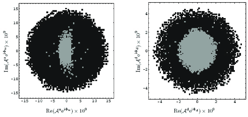
Figure 7.4: SUSY contribution to the NP amplitudes $\mathcal{A}^{u}e^{i\Phi_{u}}$ (left) and $\mathcal{A}^{d}e^{i\Phi_{d}}$ (right) in the scenario with simultaneous LL and RR mixings. The dark regions correspond to the variation of the SUSY parameters over the considered parameter space. The light regions satisfy the experimental bounds, including the recent measurement of $\Delta M_{s}$.

In Fig. 7.4 we show the allowed ranges for $\mathcal{A}^{u}e^{i\Phi_{u}}$ and $\mathcal{A}^{d}e^{i\Phi_{d}}$ in the scenario with simultaneous LL and RR mixings. The dark regions correspond to the values that these amplitudes take when varying the parameter space over the initial ranges. The light regions show how these values are reduced by the existing experimental constraints mentioned above. There are two important remarks. First, we see that the above constraints do indeed greatly reduce the allowed SUSY parameter space. Second, even so, the effect on $\mathcal{A}^{u}e^{i\Phi_{u}}$ and $\mathcal{A}^{d}e^{i\Phi_{d}}$ can be significant.

At this stage we can identify what are the effects of the various constraints in reducing the SUSY parameter space. The bound from $B\to X_{s}\gamma$ affects only the left-handed sector. In particular, for large $m_{\tilde{s}}$, the regions with $|\theta_{L}|\gtrsim 10^{\circ}$, $|\delta_{L}|\lesssim 60^{\circ}$ and $|\theta_{L}|\gtrsim 10^{\circ}$, $|\delta_{L}-\pi|\lesssim 60^{\circ}$ are excluded. The bound from $\Delta M_{s}$ is much stronger: when $m_{\tilde{s}}\gtrsim 400~{}{\rm GeV}$, any values of $|\theta_{L,R}|\gtrsim 5^{\circ}$ are excluded, as well as those regions in which $\delta_{L}+\delta_{R}\approx-3\pi/2,-\pi/2,\pi/2,3\pi/2$. After these bounds are imposed on the parameter space, the constraints from $B\to\pi K$ have very little effect on the regions in Fig. 7.4.

Note that the allowed region for $\mathcal{A}^{u}$ is much larger than that for $\mathcal{A}^{d}$, by approximately a factor of 3. In the isospin limit, these should be equal, so this factor of 3 is a measure of isospin breaking in this NP scenario. In particular, for $m_{\tilde{u}_{R}}={\rm 250~{}GeV}$ (zero $\tilde{u}_{R}$-$\tilde{d}_{R}$ mass splitting), the values of $\mathcal{A}^{u}$ reduce to those for $\mathcal{A}^{d}$.

We now examine the effect of these contributions on the observables. By adding the SUSY contributions to the SM amplitudes, it is possible to compute the branching ratio and the CP asymmetries in the presence of SUSY. Fig. 7.5 shows the allowed values for the $B_{s}^{\scriptscriptstyle 0}\to K^{+}K^{-}$ observables, for three different values of $A_{dir}^{d0}$, compared with the predictions of the SM and with the recent experimental value for the $B_{s}^{\scriptscriptstyle 0}\to K^{+}K^{-}$ branching ratio reported by the CDF collaboration [131]:

$$BR(B_{s}^{\scriptscriptstyle 0}\to K^{+}K^{-})_{\rm exp}=(24.4\pm 1.4\pm 4.6)\times 10^{-6}~{}.$$ (7.39)

The agreement between the CDF measurement and the prediction of the SM in Ref. [36] erases any discrepancy between experiment and the SM. This branching ratio will now be an important future constraint. The branching ratio within SUSY should not deviate much from the SM prediction so as not to generate any disagreement with data. Indeed, Fig. 7.5 shows that the impact of SUSY on the branching ratio of $B_{s}^{\scriptscriptstyle 0}\to K^{+}K^{-}$ is practically negligible. Interestingly, for positive values of $A_{dir}^{d0}$ (preferred region), the SM predicts a smaller value for $BR(B_{s}^{\scriptscriptstyle 0}\to K^{+}K^{-})$, but it is now compatible with the new data. Still, it is in this case that SUSY shows a larger deviation in the correct direction.

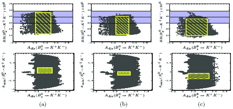
Figure 7.5: Predictions, in the form of scatter plots, for the correlations between $BR(B_{s}^{\scriptscriptstyle 0}\to K^{+}K^{-})-A_{\rm dir}(B_{s}^{\scriptscriptstyle 0}\to K^{+}K^{-})$ (up) and $A_{\rm mix}(B_{s}^{\scriptscriptstyle 0}\to K^{+}K^{-})-A_{\rm dir}(B_{s}^{\scriptscriptstyle 0}\to K^{+}K^{-})$ (down) in the presence of SUSY, for (a) $A_{dir}^{d0}=-0.1$, (b) $A_{dir}^{d0}=0$ and (c) $A_{dir}^{d0}=0.1$. The dashed rectangles correspond to the SM predictions. The horizontal band shows the experimental value for $BR(B_{s}^{\scriptscriptstyle 0}\to K^{+}K^{-})$ at $1\sigma$.

A completely different picture arises for the CP asymmetries. The results for the direct CP asymmetry reveal that SUSY can have an impact. This is not surprising: SUSY introduces a term in the total amplitude which is of the same order of magnitude as that of the SM and carries a weak phase that is not constrained. The mixing-induced CP asymmetry gets affected in a more dramatic way. The interpretation is that the SUSY contribution to the mixing angle $\phi_{s}$ can be large (in fact it can take all values between $-\pi$ and $\pi$), while in the SM it is tiny: $\phi_{s}^{SM}\simeq-2^{\circ}$. Any experimental measurement falling inside the dark area in the plots, but outside the dashed rectangle, would not only signal NP but clearly could be accommodated by supersymmetry.

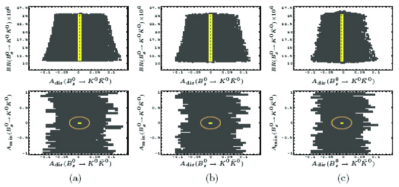
Figure 7.6: Predictions, in the form of scatter plots, for the correlations between $BR(B_{s}^{\scriptscriptstyle 0}\to K^{0}\bar{K}^{0})-A_{\rm dir}(B_{s}^{\scriptscriptstyle 0}\to K^{0}\bar{K}^{0})$ (up) and $A_{\rm mix}(B_{s}^{\scriptscriptstyle 0}\to K^{0}\bar{K}^{0})-A_{\rm dir}(B_{s}^{\scriptscriptstyle 0}\to K^{0}\bar{K}^{0})$ (down) in the presence of SUSY, for (a) $A_{dir}^{d0}=-0.1$, (b) $A_{dir}^{d0}=0$ and (c) $A_{dir}^{d0}=0.1$. The dashed rectangles correspond to the SM predictions. These are quite small in the three lower plots, so they are indicated by a circle.

Fig. 7.6 shows the results for $B_{s}^{\scriptscriptstyle 0}\to K^{0}\bar{K}^{0}$. Although the branching ratio is little changed in the presence of SUSY, the enhancement of the CP asymmetries due to the inclusion of the SUSY contributions is in this case even more important. The reason is that, within the SM, the CP asymmetries are much smaller in $B_{s}^{\scriptscriptstyle 0}\to K^{0}\bar{K}^{0}$ than they are for $B_{s}^{\scriptscriptstyle 0}\to K^{+}K^{-}$, because of the absence of the tree diagram. Thus the impact of SUSY is much greater. This is evident by looking at the three lower plots in Fig. 7.6, where the tiny rectangles corresponding to the SM predictions can hardly be observed. We have drawn a circle around them to indicate their position.

These are a good illustration of the general scenario discussed in the introduction. While the branching ratios in this case are relatively insensitive to supersymmetry, the direct and mixing-induced CP asymmetries of these decays are greatly affected. Thus, these CP asymmetries are the observables to focus on in order to observe NP, particularly SUSY, while the branching ratio of $B_{s}^{\scriptscriptstyle 0}\to K^{+}K^{-}$ can become an important constraint on models beyond the SM other than SUSY.

7.8 Summary of the results

In this chapter we have considered the branching ratios and CP asymmetries for the decays $B_{s}^{\scriptscriptstyle 0}\to K^{+}K^{-}$ and $B_{s}^{\scriptscriptstyle 0}\to K^{0}\bar{K}^{0}$ in a supersymmetric (SUSY) model, focusing on the dominant gluino-squark contributions [58]. The determination of the SM contributions has been taken from the combination of $B_{d}^{\scriptscriptstyle 0}\to K^{0}\bar{K}^{0}$ and QCD factorization described in Chapter 5 [36]. In ref. [129] the SM contributions were taken from $B_{d}\to\pi^{+}\pi^{-}$, as was done in Chapter 4 [126], but the uncertainties are much bigger. Here we have described the analysis of ref. [37]. We have also included the constraints coming from $BR(B\to X_{s}\gamma)$, $B\to\pi K$ and $\Delta M_{s}$, and we find the following results.

• The new-physics (NP) amplitudes are $\mathcal{A}^{u}e^{i\Phi_{u}}$ ($B_{s}^{\scriptscriptstyle 0}\to K^{+}K^{-}$) and $\mathcal{A}^{d}e^{i\Phi_{d}}$ ($B_{s}^{\scriptscriptstyle 0}\to K^{0}\bar{K}^{0}$). We find that both can get significant contributions from SUSY. In the isospin limit, these quantities are equal. However, our calculations show that, for the region of parameters considered, in SUSY there can be a difference of up to a factor of 3 between the NP amplitudes. This indicates the possible level of isospin breaking in this type of theory. In particular, in the SUSY model considered here, large isospin violation is possible when there is large mass splitting in $\widetilde{u}_{R}$-$\widetilde{d}_{R}$.

• The branching ratio $BR(B_{s}^{\scriptscriptstyle 0}\to K^{+}K^{-})$ is very little affected by SUSY. At most, the SM prediction can be increased by 15% for $A_{dir}^{d0}=0.1$. In fact, SUSY can somewhat improve the already good agreement between the SM prediction and the new precise CDF measurement [131]. The impact of SUSY on $BR(B_{s}^{\scriptscriptstyle 0}\to K^{0}\bar{K}^{0})$ is even smaller, reflecting the reduced allowed region for $\mathcal{A}^{d}e^{i\Phi_{d}}$ as compared to $\mathcal{A}^{u}e^{i\Phi_{u}}$.

• The situation is very different for the CP asymmetries; the size of the effect depends strongly on the decay and the type of asymmetry. For $B_{s}^{\scriptscriptstyle 0}\to K^{+}K^{-}$, the direct CP asymmetry within SUSY is in the range $-0.1\lesssim A_{dir}(B_{s}^{\scriptscriptstyle 0}\to K^{+}K^{-})^{SUSY}\lesssim 0.7$ for $-0.1\leq A_{dir}^{d0}\leq 0.1$. Depending on the value of $A_{dir}^{d0}$, it may be possible to disentangle the SUSY contribution from that of the SM. This is due to the competition between the tree and the NP amplitudes for each value of $A_{dir}^{d0}$. As for $A_{mix}(B_{s}^{\scriptscriptstyle 0}\to K^{+}K^{-})$, its value can vary all the way from $-1$ to $+1$, signaling a large impact from SUSY.

• Turning to $B_{s}^{\scriptscriptstyle 0}\to K^{0}\bar{K}^{0}$, the CP asymmetries are particularly promising. This decay is dominated by the penguin amplitude in the SM, and so the direct CP asymmetry is strongly suppressed: it is predicted to be at most of the order of 1%. However, in the presence of SUSY, the direct CP asymmetry can be 10 times larger. The mixing-induced CP asymmetry is also predicted to be very small in the SM. However, $A_{mix}(B_{s}^{\scriptscriptstyle 0}\to K^{0}\bar{K}^{0})^{SUSY}$ covers the entire range, and so this asymmetry can be large in the presence of SUSY.

Part III Conclusions

Chapter 8 Concluding Remarks

Non-leptonic weak decays of B mesons are suitable for the combined study of different aspects in the phenomenology of particle physics. We have seen their relevance in studies of CP violation, strong interactions, heavy quark physics, flavor physics and physics beyond the SM. All these topics are interconnected and related to the search for new physics; a search that will most probably succeed in the next few years, but with consequences that will surely require theoretical and experimental work for a much longer time.

This is a very interesting moment in the history of particle physics, in which we expect to finally break the TeV wall and go beyond a theory of elementary particles formulated forty years ago. The outcome can be a completely new understanding of the world we live in, leaving aside the period of speculation and uncertainty of the last decades. A joint effort of the whole particle physics community has brought us here, and the same effort will be necessary to make this breakthrough possible. It is an impressive world-wide project that will have a historic result.

The direct search for new particles is a crucial part of this program. The main objective of the LHC, with its experiments ATLAS and CMS, is to find the elusive higgs particle, the last requirement of the SM. However, a more important task will be the search for other completely new particles that might help to understand all the puzzles that the SM leaves unanswered. In fact, from the theoretical point of view, the observation of new particles might be much more valuable than the establishment of the higgs’ existence.

Despite the importance of the direct searches, the correct identification of the new physics and its properties, and the understanding of its theoretical consequences, requires also from indirect analyses. Some of the major open questions in particle physics that might find a partial answer in the next future experiments are related to flavor physics. B physics has been the center of attention in the experiments of the last decade, with a huge amount of data collected at the B factories and at Tevatron, and will keep a place of honor in the future, with the B physics experiment LHCb at the LHC and a future Super B. The reason for this is that B physics is a powerful probe of physics beyond the SM in a completely complementary way to direct searches. In fact, all the B physics experiments carried out so far have put stringent bounds on the nature of the new physics, so thus far the indirect searches are on the head of the list. And whether or not the direct production of new particles takes place, B physics will still be an important way to test the SM and look for new physics.

However, in order to look for tiny new physics effects, the SM predictions must be under strict control. In this thesis we have focused on non-leptonic B decays. These type of decays are very difficult to study because of their sensitivity to long distance strong interaction effects. So in order to look for new physics in these decays one must find a way to deal with hadronic phenomena leading to predictions of acceptable accuracy. Indeed, the claim of a NP signal in non-leptonic B decays will have to rely on a solid inclusion of long distance QCD contributions. This also means that the study of these decays might have a double prize: understanding the NP, and understanding QCD. We have already obtained benefits from both sides.

Towards this end, we have presented analyses of two body non-leptonic B decays within two approaches. The first one is the flavor symmetry approach, which takes advantage of the approximate $SU(3)$ symmetry of the QCD lagrangian to establish relations between hadronic quantities for different decay modes, in such a way that predictions can be made without the need of direct computations of these hadronic quantities. One can then use data on some sort to predict the values of other observables. In Chapter 4 we have used this approach to extract the SM hadronic parameters in $B_{s}\to K^{+}K^{-}$ decays from $B_{d}\to\pi^{+}\pi^{-}$ data. This has provided predictions for $B_{s}\to K^{+}K^{-}$ observables within the SM that can be compared with experiment. A deviation between the theoretical predictions and the experimental data will be a signal of NP. A useful general parametrization of the NP contributions to this decay has been given, together with a method to measure the new physics parameters. Therefore, if NP was found in this decay, the measurement of these NP parameters would provide interesting information on the nature of this NP, as for example if the NP is isospin violating, and so on. The limitations of the $SU(3)$ analysis have been discussed in detail, in particular the problem of estimating the symmetry breaking effects, that constitute the main source of uncertainties.

A second approach that has been discussed here is the QCD factorization method. This provides a tool to compute matrix elements from first principles, based on a heavy quark expansion. Therefore this approach provides genuine QCD predictions. However, some of the phenomenological difficulties of this approach are those non-factorizable power suppressed contributions that are numerically important for realistic $b$ quark masses. In Chapter 5 we have proposed a method to get around this difficulty. A combination of QCDF with flavor symmetry relations has been used to study $B_{s}\to KK$ decays, giving predictions for the observables with uncertainties reduced by more than a $50\%$. This method has also been used in Chapter 6 for $B_{s}\to VV$ decays, and used to propose three strategies to measure the $B_{s}-\bar{B_{s}}$ mixing angle. This mixing angle is predicted to be extremely small within the SM, and it is therefore an excellent place to look for NP. However, the claim of a NP contribution to this mixing angle cannot be easily disentangled from a NP contribution to the decay amplitudes in these type of decays, and we have discussed the ways in which these strategies could help to make this distinction.

This proposal is clearly an improvement on the flavor symmetry and the QCDF approaches, giving more reliable results with smaller uncertainties. In fact, the results presented for $B_{s}\to K^{+}K^{-}$ were predictions that were confirmed very nicely –maybe unfortunately– by the CDF collaboration shortly after. We would like to make some further comments concerning this method. The applicability of the approach has to be checked individually for each mode: it can only be applied to those decays for which $\Delta$ receives no contributions from annihilation or hard spectator scattering graphs, such as $B\to K^{(*)}K^{(*)}$, $B_{d}\to\phi K^{(*)}$, $B^{+}\to\pi^{+}\phi$, etc, as discussed in Section 5.1. The predictions derived in this way include most of the long distance physics, which is contained inside the experimental input. The used theoretical input is minimal, and is the most reliable input that QCDF can offer, free from the troublesome IR-divergencies. Moreover, the theoretical error is under control and is likely to be reduced in the near future due to, for example, the fast progress that is taking place in lattice simulations.

There is, however, an honest criticism due to the fact that some long distance effects that are controversial in QCDF, are also absent here. The prominent one is the contribution from the charming penguins, which could easily account for a significant discrepancy between theory and experiment that would not be due to NP.

Finally, in Chapter 7 we have studied $B_{s}\to KK$ decays in supersymmetry. Using the SM analyses performed in the previous chapters, and computing the most relevant contributions from SUSY to the decay amplitudes and to the mixing, we have studied the departure from SM expectations that SUSY could provide in the branching ratios and CP asymmetries. The conclusion is that the enhancements are important, which means that moderately precise experimental measurements on these observables, if consistent with the SM predictions, will provide useful constraints on the SUSY parameter space, especially on the CP violating phases.

To be able foresee what is the most relevant direction that future work on these topics should follow requires a considerable scientific maturity, which I lack. However, there are some general aspects concerning this issue that are of a general opinion.

On the QCD side, an all-order proof of factorization within QCDF would be appealing, but maybe not too useful for practical purposes. A further development of the SCET formulation will probably put factorization theorems on a much more firm basis, specially if the issue of the long distance charm loops finds a phenomenologically satisfactory solution. The final aim is to have a completely systematic way to compute QCD corrections to matrix elements up to any desired accuracy (even if it means that the actual computation is extremely difficult and lengthy). Moreover, a similar progress should be expected from the lattice community, which is certainly conceivable.

On the NP side, the progress should be faster, since immediate future events will have a drastic influence on any work in this direction. The SM fits are almost completely systematized, and any tension between theory and experiment can be dragged to the origin with ease. Probably a similar systematization should be built for the largest possible of phenomenologically relevant NP models that exist in the literature, so that the explosion of new phenomena that might occur in the first five years at the LHC can be used to accept and discard models in the blink of an eye.

However, the true model of particle physics at the TeV scale might have nothing to do with any of the NP models that have been proposed up to now. Therefore, model-independent studies of NP are necessary in order to be sure that we are not missing anything new, or old.

Bibliography

- [1]
- [2] M. Neubert, Phys. Rept. 245, 259 (1994) [arXiv:hep-ph/9306320].
- [3] C. W. Bauer, S. Fleming and M. E. Luke, Phys. Rev. D 63, 014006 (2001) [arXiv:hep-ph/0005275].
- [4] C. W. Bauer, S. Fleming, D. Pirjol and I. W. Stewart, Phys. Rev. D 63, 114020 (2001) [arXiv:hep-ph/0011336].
- [5] C. W. Bauer, D. Pirjol and I. W. Stewart, Phys. Rev. D 65, 054022 (2002) [arXiv:hep-ph/0109045].
- [6] M. Beneke, A. P. Chapovsky, M. Diehl and T. Feldmann, Nucl. Phys. B 643, 431 (2002) [arXiv:hep-ph/0206152].
- [7] J. Chay and C. Kim, Phys. Rev. D 65, 114016 (2002) [arXiv:hep-ph/0201197].
- [8] R. J. Hill and M. Neubert, Nucl. Phys. B 657, 229 (2003) [arXiv:hep-ph/0211018].
- [9] G. Buchalla, A. J. Buras and M. E. Lautenbacher, Rev. Mod. Phys. 68, 1125 (1996) [arXiv:hep-ph/9512380].
- [10] A. J. Buras, arXiv:hep-ph/9806471.
- [11] G. Buchalla, G. Hiller, Y. Nir and G. Raz, JHEP 0509, 074 (2005) [arXiv:hep-ph/0503151].
- [12] W. Buchmuller and D. Wyler, Nucl. Phys. B 268, 621 (1986).
- [13] A. J. Buras, Acta Phys. Polon. B 34, 5615 (2003) [arXiv:hep-ph/0310208].
- [14] L. J. Hall and L. Randall, Phys. Rev. Lett. 65, 2939 (1990).
- [15] M. Neubert and B. Stech, Adv. Ser. Direct. High Energy Phys. 15, 294 (1998) [arXiv:hep-ph/9705292].
- [16] A. J. Buras and L. Silvestrini, Nucl. Phys. B 548, 293 (1999) [arXiv:hep-ph/9806278].
- [17] H. Y. Cheng, Phys. Lett. B 335, 428 (1994) [arXiv:hep-ph/9406262].
- [18] H. Y. Cheng and B. Tseng, Phys. Rev. D 58, 094005 (1998) [arXiv:hep-ph/9803457].
- [19] A. Ali and C. Greub, Phys. Rev. D 57, 2996 (1998) [arXiv:hep-ph/9707251].
- [20] A. Ali, G. Kramer and C. D. Lu, Phys. Rev. D 58, 094009 (1998) [arXiv:hep-ph/9804363].
- [21] H. Y. Cheng, H. n. Li and K. C. Yang, Phys. Rev. D 60, 094005 (1999) [arXiv:hep-ph/9902239].
- [22] M. Beneke, G. Buchalla, M. Neubert and C. T. Sachrajda, Phys. Rev. Lett. 83, 1914 (1999) [arXiv:hep-ph/9905312].
- [23] M. Beneke, G. Buchalla, M. Neubert and C. T. Sachrajda, Nucl. Phys. B 591, 313 (2000) [arXiv:hep-ph/0006124].
- [24] M. Beneke, G. Buchalla, M. Neubert and C. T. Sachrajda, Nucl. Phys. B 606, 245 (2001) [arXiv:hep-ph/0104110].
- [25] D. s. Du, D. s. Yang and G. h. Zhu, Phys. Rev. D 64, 014036 (2001) [arXiv:hep-ph/0103211].
- [26] D. s. Du, H. j. Gong, J. f. Sun, D. s. Yang and G. h. Zhu, Phys. Rev. D 65, 094025 (2002) [Erratum-ibid. D 66, 079904 (2002)] [arXiv:hep-ph/0201253].
- [27] M. Beneke and M. Neubert, Nucl. Phys. B 675, 333 (2003) [arXiv:hep-ph/0308039].
- [28] M. Beneke, J. Rohrer and D. Yang, Nucl. Phys. B 774, 64 (2007) [arXiv:hep-ph/0612290].
- [29] M. Beneke and T. Feldmann, Nucl. Phys. B 592, 3 (2001) [arXiv:hep-ph/0008255].
- [30] A. L. Kagan, Phys. Lett. B 601, 151 (2004) [arXiv:hep-ph/0405134].
- [31] V. M. Braun and I. E. Filyanov, Z. Phys. C 44, 157 (1989) [Sov. J. Nucl. Phys. 50, 511.1989 YAFIA,50,818 (1989 YAFIA,50,818-830.1989)].
- [32] V. M. Braun and I. E. Filyanov, Sov. J. Nucl. Phys. 52, 126 (1990) [Z. Phys. C 48, 239 (1990 YAFIA,52,199-213.1990)].
- [33] C. W. Bauer, D. Pirjol and I. W. Stewart, Phys. Rev. Lett. 87, 201806 (2001) [arXiv:hep-ph/0107002].
- [34] J. D. Bjorken, Nucl. Phys. Proc. Suppl. 11, 325 (1989).
- [35] M. Bander, D. Silverman and A. Soni, Phys. Rev. Lett. 43, 242 (1979).
- [36] S. Descotes-Genon, J. Matias and J. Virto, Phys. Rev. Lett. 97, 061801 (2006) [arXiv:hep-ph/0603239].
- [37] S. Baek, D. London, J. Matias and J. Virto, JHEP 0612, 019 (2006) [arXiv:hep-ph/0610109].
- [38] A. Datta, M. Imbeault, D. London and J. Matias, Phys. Rev. D 75, 093004 (2007) [arXiv:hep-ph/0611280].
- [39] S. Descotes-Genon, J. Matias and J. Virto, Phys. Rev. D 76, 074005 (2007) [arXiv:0705.0477 [hep-ph]].
- [40] J. Virto, AIP Conf. Proc. 964, 90 (2007) [arXiv:0707.2046 [hep-ph]].
- [41] M. Ciuchini, E. Franco, G. Martinelli and L. Silvestrini, Nucl. Phys. B 501, 271 (1997) [arXiv:hep-ph/9703353].
- [42] M. Ciuchini, E. Franco, G. Martinelli, M. Pierini and L. Silvestrini, Phys. Lett. B 515, 33 (2001) [arXiv:hep-ph/0104126].
- [43] C. W. Bauer, D. Pirjol, I. Z. Rothstein and I. W. Stewart, Phys. Rev. D 70, 054015 (2004) [arXiv:hep-ph/0401188].
- [44] M. Beneke, G. Buchalla, M. Neubert and C. T. Sachrajda, Phys. Rev. D 72, 098501 (2005) [arXiv:hep-ph/0411171].
- [45] A. Jain, I. Z. Rothstein and I. W. Stewart, arXiv:0706.3399 [hep-ph].
- [46] S. Weinberg, Phys. Rev. D 11, 3583 (1975).
- [47] G. ’t Hooft, Phys. Rev. Lett. 37, 8 (1976).
- [48] A. Khodjamirian, T. Mannel and M. Melcher, Phys. Rev. D 68, 114007 (2003) [arXiv:hep-ph/0308297].
- [49] M. Gronau, Phys. Lett. B 265, 389 (1991).
- [50] Y. Nir and H. R. Quinn, Phys. Rev. Lett. 67, 541 (1991).
- [51] H. J. Lipkin, Y. Nir, H. R. Quinn and A. Snyder, Phys. Rev. D 44, 1454 (1991).
- [52] J. J. de Swart, Rev. Mod. Phys. 35, 916 (1963).
- [53] B. Grinstein and R. F. Lebed, Phys. Rev. D 53, 6344 (1996) [arXiv:hep-ph/9602218].
- [54] M. Gronau, O. F. Hernandez, D. London and J. L. Rosner, Phys. Rev. D 50, 4529 (1994) [arXiv:hep-ph/9404283].
- [55] M. Gronau, O. F. Hernandez, D. London and J. L. Rosner, Phys. Rev. D 52, 6374 (1995) [arXiv:hep-ph/9504327].
- [56] M. Gronau, Y. Grossman, G. Raz and J. L. Rosner, Phys. Lett. B 635, 207 (2006) [arXiv:hep-ph/0601129].
- [57] R. Escribano, J. Matias and J. Virto, arXiv:0708.0119 [hep-ph].
- [58] Y. Grossman, M. Neubert and A. L. Kagan, JHEP 9910, 029 (1999) [arXiv:hep-ph/9909297].
- [59] M. Neubert, JHEP 9902, 014 (1999) [arXiv:hep-ph/9812396].
- [60] M. J. Savage and M. B. Wise, Phys. Rev. D 39, 3346 (1989) [Erratum-ibid. D 40, 3127 (1989)].
- [61] R. Fleischer and T. Mannel, Phys. Rev. D 57, 2752 (1998) [arXiv:hep-ph/9704423].
- [62] A. J. Buras, R. Fleischer and T. Mannel, Nucl. Phys. B 533, 3 (1998) [arXiv:hep-ph/9711262].
- [63] Y. Grossman, G. Isidori and M. P. Worah, Phys. Rev. D 58, 057504 (1998) [arXiv:hep-ph/9708305].
- [64] M. Neubert and J. L. Rosner, Phys. Lett. B 441, 403 (1998) [arXiv:hep-ph/9808493].
- [65] R. Fleischer, Phys. Lett. B 459, 306 (1999) [arXiv:hep-ph/9903456].
- [66] Y. Grossman, Z. Ligeti, Y. Nir and H. Quinn, Phys. Rev. D 68, 015004 (2003) [arXiv:hep-ph/0303171].
- [67] J. Matias, Phys. Lett. B 520, 131 (2001) [arXiv:hep-ph/0105103].
- [68] C. S. Wu, E. Ambler, R. W. Hayward, D. D. Hoppes and R. P. Hudson, Phys. Rev. 105, 1413 (1957).
- [69] R. L. Garwin, L. M. Lederman and M. Weinrich, Phys. Rev. 105, 1415 (1957).
- [70] M. Gell-Mann and A. Pais, Phys. Rev. 97, 1387 (1955).
- [71] J. H. Christenson, J. W. Cronin, V. L. Fitch and R. Turlay, Phys. Rev. Lett. 13, 138 (1964).
- [72] W. M. Yao et al. [Particle Data Group], J. Phys. G 33, 1 (2006).
- [73] M. Kobayashi and T. Maskawa, Prog. Theor. Phys. 49, 652 (1973).
-
[74]
M. Bona et al. [UTfit Collaboration],
JHEP 0610, 081 (2006);
http://utfit.roma1.infn.it/. -
[75]
J. Charles et al. [CKMfitter Group],
Eur. Phys. J. C 41, 1 (2005);
http://ckmfitter.in2p3.fr/. - [76] A. D. Sakharov, Pisma Zh. Eksp. Teor. Fiz. 5, 32 (1967) [JETP Lett. 5, 24 (1967 SOPUA,34,392-393.1991 UFNAA,161,61-64.1991)].
- [77] V. L. Fitch, P. A. Piroué and R. B. Perkins, Nuovo Cim. 22 1160 (1961).
- [78] C. Albajar et al. [UA1 Collaboration], Phys. Lett. B 186, 247 (1987) [Erratum-ibid. 197B, 565 (1987)].
- [79] H. Albrecht et al. [ARGUS COLLABORATION Collaboration], Phys. Lett. B 192, 245 (1987).
- [80] A. Abulencia et al. [CDF - Run II Collaboration], Phys. Rev. Lett. 97, 062003 (2006) [AIP Conf. Proc. 870, 116 (2006)] [arXiv:hep-ex/0606027].
- [81] B. Aubert et al. [BABAR Collaboration], Phys. Rev. Lett. 98, 211802 (2007) [arXiv:hep-ex/0703020].
- [82] V. Weisskopf and E. P. Wigner, Z. Phys. 63, 54 (1930).
- [83] T. D. Lee and L. Wolfenstein, Phys. Rev. 138, B1490 (1965).
- [84] I. I. Y. Bigi and A. I. Sanda, Camb. Monogr. Part. Phys. Nucl. Phys. Cosmol. 9, 1 (2000).
- [85] P. F. . Harrison and H. R. . Quinn [BABAR Collaboration],
- [86] E. Barberio et al. [Heavy Flavor Averaging Group (HFAG) Collaboration], arXiv:0704.3575 [hep-ex]; http://www.slac.stanford.edu/xorg/hfag/.
- [87] A. Abulencia et al. [CDF Collaboration], Phys. Rev. Lett. 97, 242003 (2006) [arXiv:hep-ex/0609040].
- [88] I. I. Y. Bigi and A. I. Sanda, Nucl. Phys. B 193, 85 (1981).
- [89] H. Boos, T. Mannel and J. Reuter, Phys. Rev. D 70, 036006 (2004) [arXiv:hep-ph/0403085].
- [90] M. Ciuchini, M. Pierini and L. Silvestrini, Phys. Rev. Lett. 95, 221804 (2005) [arXiv:hep-ph/0507290].
- [91] H. n. Li and S. Mishima, JHEP 0703, 009 (2007) [arXiv:hep-ph/0610120].
- [92] S. L. Glashow, Nucl. Phys. 22, 579 (1961).
- [93] S. Weinberg, Phys. Rev. Lett. 19, 1264 (1967).
- [94] A. Salam, in Elementary Particle Theory, ed. N. Savartholm (Almquist and Wiksells, Stockholm, 1969), p.367.
- [95] N. Cabibbo, Phys. Rev. Lett. 10, 531 (1963).
- [96] L. L. Chau and W. Y. Keung, Phys. Rev. Lett. 53, 1802 (1984).
- [97] L. Wolfenstein, Phys. Rev. Lett. 51, 1945 (1983).
- [98] M. E. Peskin and D. V. Schroeder, Reading, USA: Addison-Wesley (1995) 842 p
- [99] P. Ball, J. M. Frere and J. Matias, Nucl. Phys. B 572, 3 (2000) [arXiv:hep-ph/9910211].
- [100] N. Arkani-Hamed, G. L. Kane, J. Thaler and L. T. Wang, JHEP 0608, 070 (2006) [arXiv:hep-ph/0512190].
- [101] A. Datta and D. London, Phys. Lett. B 595, 453 (2004) [arXiv:hep-ph/0404130].
- [102] M. Gronau, O. F. Hernandez, D. London and J. L. Rosner, Phys. Rev. D 52, 6356 (1995) [arXiv:hep-ph/9504326].
- [103] B. Aubert et al. [BaBar Collaboration], Phys. Rev. Lett. 95, 151803 (2005) [arXiv:hep-ex/0501071].
- [104] Y. Chao et al. [Belle Collaboration], Phys. Rev. D 69, 111102 (2004) [arXiv:hep-ex/0311061].
- [105] K. Abe et al. [Belle Collaboration], Phys. Rev. Lett. 95, 101801 (2005) [arXiv:hep-ex/0502035].
- [106] A. J. Buras, R. Fleischer, S. Recksiegel and F. Schwab, Acta Phys. Polon. B 36, 2015 (2005) [arXiv:hep-ph/0410407].
- [107] Y. F. Zhou, Eur. Phys. J. C 46, 713 (2006) [arXiv:hep-ph/0507126].
- [108] S. Baek, JHEP 0607, 025 (2006) [arXiv:hep-ph/0605094].
- [109] Y. L. Wu, Y. F. Zhou and C. Zhuang, Phys. Rev. D 74, 094007 (2006) [arXiv:hep-ph/0609006].
- [110] A. J. Buras, R. Fleischer, S. Recksiegel and F. Schwab, Eur. Phys. J. C 32, 45 (2003) [arXiv:hep-ph/0309012].
- [111] A. J. Buras, R. Fleischer, S. Recksiegel and F. Schwab, Phys. Rev. Lett. 92, 101804 (2004) [arXiv:hep-ph/0312259].
- [112] A. J. Buras, R. Fleischer, S. Recksiegel and F. Schwab, Nucl. Phys. B 697, 133 (2004) [arXiv:hep-ph/0402112].
- [113] A. J. Buras, R. Fleischer, S. Recksiegel and F. Schwab, Eur. Phys. J. C 45, 701 (2006) [arXiv:hep-ph/0512032].
- [114] R. Fleischer, Int. J. Mod. Phys. A 21, 664 (2006) [arXiv:hep-ph/0507156].
- [115] R. Fleischer, J. Phys. G 32, R71 (2006) [arXiv:hep-ph/0512253].
- [116] Y. L. Wu and Y. F. Zhou, Phys. Rev. D 72, 034037 (2005) [arXiv:hep-ph/0503077].
- [117] C. W. Chiang and Y. F. Zhou, JHEP 0612, 027 (2006) [arXiv:hep-ph/0609128].
- [118] A. Datta and D. London, Int. J. Mod. Phys. A 19, 2505 (2004) [arXiv:hep-ph/0303159].
- [119] B. Aubert et al. [BABAR Collaboration], Phys. Rev. Lett. 93, 231804 (2004) [arXiv:hep-ex/0408017].
- [120] K. Senyo [BELLE Collaboration], arXiv:hep-ex/0505067.
- [121] B. Aubert et al. [BABAR Collaboration], Phys. Rev. Lett. 91, 171802 (2003) [arXiv:hep-ex/0307026].
- [122] K. F. Chen et al. [BELLE Collaboration], Phys. Rev. Lett. 94, 221804 (2005) [arXiv:hep-ex/0503013].
- [123] J. Zhang et al. [BELLE Collaboration], arXiv:hep-ex/0505039.
- [124] S. Baek, A. Datta, P. Hamel, O. F. Hernandez and D. London, Phys. Rev. D 72, 094008 (2005) [arXiv:hep-ph/0508149].
- [125] D. London and J. Matias, Phys. Rev. D 70, 031502 (2004) [arXiv:hep-ph/0404009].
- [126] D. London, J. Matias and J. Virto, Phys. Rev. D 71, 014024 (2005) [arXiv:hep-ph/0410011].
- [127] R. Fleischer and J. Matias, Phys. Rev. D 61, 074004 (2000) [arXiv:hep-ph/9906274].
- [128] R. Fleischer and J. Matias, Phys. Rev. D 66, 054009 (2002) [arXiv:hep-ph/0204101].
- [129] S. Baek, D. London, J. Matias and J. Virto, JHEP 0602, 027 (2006) [arXiv:hep-ph/0511295].
- [130] M. Beneke, In the Proceedings of 2nd Workshop on the CKM Unitarity Triangle, Durham, England, 5-9 Apr 2003, pp FO001 [arXiv:hep-ph/0308040].
- [131] G. Cynolter and E. Lendvai, J. Phys. G 34, 1711 (2007) [arXiv:hep-ph/0607021].
- [132] A. Abulencia et al. [CDF Collaboration], Phys. Rev. Lett. 97, 211802 (2006) [arXiv:hep-ex/0607021].
- [133] B. Aubert et al. [BABAR Collaboration], Phys. Rev. Lett. 97, 171805 (2006) [arXiv:hep-ex/0608036].
- [134] B. Kayser, M. Kuroda, R. D. Peccei and A. I. Sanda, Phys. Lett. B 237, 508 (1990).
- [135] C. Sharma and R. Sinha, Phys. Rev. D 73, 014016 (2006) [arXiv:hep-ph/0504178].
- [136] C. W. Chiang, Phys. Rev. D 62, 014017 (2000) [arXiv:hep-ph/0002243].
- [137] J. Matias, Acta Phys. Polon. B 38, 2901 (2007) [arXiv:hep-ph/0701116].
- [138] A. S. Dighe, I. Dunietz and R. Fleischer, Eur. Phys. J. C 6, 647 (1999) [arXiv:hep-ph/9804253].
- [139] A. Datta, M. Imbeault, D. London, V. Page, N. Sinha and R. Sinha, Phys. Rev. D 71, 096002 (2005) [arXiv:hep-ph/0406192].
- [140] R. Fleischer, Eur. Phys. J. C 33, S268 (2004) [arXiv:hep-ph/0310081].
- [141] R. Fleischer, Nucl. Phys. B 671, 459 (2003) [arXiv:hep-ph/0304027].
- [142] M. Bona et al., arXiv:0709.0451 [hep-ex].
- [143] J. S. Hagelin, S. Kelley and T. Tanaka, Nucl. Phys. B 415, 293 (1994).
- [144] D. Becirevic et al., Nucl. Phys. B 634, 105 (2002) [arXiv:hep-ph/0112303].
- [145] D. Becirevic, V. Gimenez, G. Martinelli, M. Papinutto and J. Reyes, JHEP 0204, 025 (2002) [arXiv:hep-lat/0110091].
- [146] A. L. Kagan and M. Neubert, Eur. Phys. J. C 7, 5 (1999) [arXiv:hep-ph/9805303].
- [147] S. Baek, JHEP 0609, 077 (2006) [arXiv:hep-ph/0605182].