DESY-07-206

We regularise the 3d $\lambda\phi^{4}$ model by discretising the Euclidean time and representing the spatial part on a fuzzy sphere. The latter involves a truncated expansion of the field in spherical harmonics. This yields a numerically tractable formulation, which constitutes an unconventional alternative to the lattice. In contrast to the 2d version, the radius $R$ plays an independent rôle. We explore the phase diagram in terms of $R$ and the cutoff, as well as the parameters $m^{2}$ and $\lambda$. Thus we identify the phases of disorder, uniform order and non-uniform order. We compare the result to the phase diagrams of the 3d model on a non-commutative torus, and of the 2d model on a fuzzy sphere. Our data at strong coupling reproduce accurately the behaviour of a matrix chain, which corresponds to the $c=1$–model in string theory. This observation enables a conjecture about the thermodynamic limit.

1 Introduction

A variety of approaches to the regularisation of quantum field theory exist. Dimensional regularisation [1] is most popular in the framework of perturbation theory. In order to overcome the limitations of a perturbative expansion, however, a regularisation should restrict the formulation to a finite set of degrees of freedom. If the Euclidean action is real and bounded from below, a model can then be treated numerically as a statistical system. This method provides in many cases the only access to observables beyond perturbation theory or semi-classical approximations.

From a general perspective, field theoretic models start from some algebra ${\cal A}$ for functions on a manifold ${\cal M}$, and a differential operator ${\cal D}$ with its Hilbert space ${\cal H}$. The standard approach for non-perturbative studies discretises the manifold to a lattice. Then the degrees of freedom to work with are usually the field variables on the lattice sites or links (see e.g. Ref. [2]). As an alternative, also Monte Carlo simulations employing the fields at discrete momenta have been suggested [3], though much less explored. In both cases ${\cal M}$ is reduced to a finite lattice.

Generally the goal is to approximate a triple $({\cal A},{\cal H},{\cal D})$ [4]. This might be achieved in quite abstract ways, but in practice a physical picture for the regularised system is a useful guide-line. In the lattice formulation one approximates the entire triple. The algebra is approximated by a commutative algebra on a lattice of points which discretise ${\cal M}$, while the differential operator is obtained by a finite difference approximation to ${\cal D}$, and the Hilbert space is adapted to this operator.

Here we are concerned with an alternative scheme, which is endowed with a physical picture on the regularised level as well. Instead of the discrete eigenvalues of the space-time or momentum coordinates, we now deal with angular momentum coordinates. To this end the fields are wrapped on a sphere and expanded in spherical harmonics. A related idea occurred already in an early construction of a non-commutative space, which added an extra dimension and preserved 5d Lorentz symmetry [5]. This method benefits from the natural discretisation of angular momentum space in quantum physics, but a cutoff still has to be imposed. In the interpretation of the angular momenta as spherical coordinates, the cutoff renders the sphere fuzzy. These coordinates are embedded in matrices, which are Hermitian in the case of the neutral scalar field to be considered here.

The concept of a fuzzy sphere regularisation has been established in Refs. [6]. The Laplace-Beltrami operator ${\cal D}^{2}$ is given in terms of angular momentum operators, which are expressed by $N$-dimensional irreducible representations of $SU(2)$. The algebra ${\cal A}$ is expanded in the polarisation tensors, which are matrix analogues of the spherical harmonics [7]. In contrast to the lattice, this regularisation does not explicitly break the space symmetries. Its analytic properties have been studied extensively in recent years, but the applicability in numerical simulations is less explored. The questions are if such simulations are feasible and to what kind of limits the measured observables can be extrapolated. So far the 2d $\lambda\phi^{4}$ model has been investigated in this respect [8]. Here we extend this study to three dimensions, where the spatial plane is mapped onto a fuzzy sphere, and the Euclidean time is lattice discretised. This extension entails qualitative differences, which are essential in view of the prospects of proceeding to four dimensions. In particular the radius $R$ of the sphere plays an independent rôle (it cannot be absorbed by simple rescaling). The recovery of a flat space without truncation requires the limits $N,\,R\to\infty$.

Section 2 presents the fuzzy sphere formulation of the $\lambda\phi^{4}$ model, along with suitable order parameters. The identification of the phase transitions in the $(\lambda,m^{2})$-plane is described in Section 3. Section 4 discusses the scaling of the phase transition lines in terms of $N$ and $R$. Section 5 compares our results to the phase diagram of the corresponding 2d model on a fuzzy sphere, and to the model on a 3d non-commutative torus. We also demonstrate that our data at strong coupling agree with the behaviour of a matrix chain model, which attracted interest in string theory. This observation allows for a conjecture about the large $N$ extrapolation, as we point out in Section 6. Our results are summarised in Section 7, and technicalities of the simulation are added in an Appendix.

A synopsis of this work has been anticipated in a proceeding contribution [10], and details are presented in a Ph.D. thesis [11].

2 The fuzzy sphere formulation of the 3d $\lambda\phi^{4}$ model

2.1 Regularisation

In this subsection we specify the regularisation that we used in our simulations. The theory to be regularised is the $\lambda\phi^{4}$ model in 3 dimensions, where we assume periodic boundary conditions in the Euclidean time $t\,$, and the space is taken as a sphere in ${\kern 2.5pt\sf{R}\kern-7.79999pt\sf{I}\kern 7.79999pt\kern-2.5pt}^{3}$. Thus the action reads

$$S[\phi]=\int_{0}^{T}dt\int d^{3}x\,\delta(\vec{x}^{\,2}-R^{2})\ \Big{[}\frac{1}{2}\phi\Big{(}-\partial_{t}^{2}+\frac{{\cal L}^{2}}{R^{2}}\Big{)}\phi+\frac{m^{2}}{2}\phi^{2}+\frac{\lambda}{4}\phi^{4}\Big{]}\ .$$ (2.1)

$T$ is the temporal periodicity and $R$ is the radius of the sphere, which we are going to denote by $S_{R}^{2}\,$. $\phi(t,\vec{x})\in{\kern 2.5pt\sf{R}\kern-7.79999pt\sf{I}\kern 7.79999pt\kern-2.5pt}$ is a scalar field and ${\cal L}^{2}=\sum_{i=1}^{3}{\cal L}_{i}^{2}\,$, ${\cal L}_{i}$ being the angular momentum components.

For the regularisation in time we introduce $N_{t}$ equidistant sites and replace $\partial_{t}$ by the standard lattice derivative. We are going to use lattice units, i.e. we set $N_{t}=T$. Thus a configuration is given by a set $\phi_{t}(\vec{x})\,$, $t=1,\dots,N_{t}\,$.

Our regularisation of the sphere $S_{R}^{2}$ is less standard, but it also relies on a concept established in the literature [6]. The coordinates $x_{i}$ are replaced by operators $X_{i}$, which still obey the constraint

$$\sum_{i=1}^{3}X_{i}^{2}=R^{2}\cdot 1\!\!1\ .$$ (2.2)

A truncation to a maximal angular momentum $\ell_{\rm max}$ means that the operators $X_{i}$ take the form of $N\times N$ matrices with $N=\ell_{\max}+1$,

$$X_{i}=\frac{2R}{\sqrt{N^{2}-1}}\,L_{i}\ ,\qquad(X_{i}\in{\rm Mat}_{N})\ .$$ (2.3)

The $L_{i}$ are generators in an $N$-dimensional irreducible representation of $SU(2)$. These coordinate operators do not commute,

$$[X_{i},X_{j}]={\rm i}\,\frac{2R}{\sqrt{N^{2}-1}}\,\epsilon_{ijk}X_{k}\ .$$ (2.4)

Thus they cannot describe sharp points; the sphere becomes fuzzy.

A scalar field, which can be expressed as a power series in the coordinates, now turns into an expansion in the operators $X_{i}$ (at some fixed time site $t$). Thus this formulation represents the field by $N\times N$ matrices $\Phi_{t}$. In particular for the neutral scalar field these matrices are Hermitian. Its spatial derivatives are given as commutators, $\partial_{i}\phi_{t}(\vec{x})\to{\rm i}\,[L_{i},\Phi_{t}]\,$.

In summary, the recipe for the regularisation from a sharp to a fuzzy sphere involves the replacements

$$x_{i}\in S_{R}^{2} \rightarrow X_{i}\in{\rm Mat}_{N}$$

$$\phi_{t}(\vec{x})\in C^{\infty}(S_{R}^{2}) \rightarrow \Phi_{t}\in{\rm Mat}_{N}\qquad{\rm(Hermitian)}$$

$${\cal L}^{2}\phi_{t}(\vec{x}) \rightarrow \hat{\cal L}^{2}\Phi_{t}:=\sum_{i=1}^{3}\,[L_{i},[L_{i},\Phi_{t}]]$$

$$\frac{1}{4\pi R^{2}}\int_{S_{R}^{2}}d\Omega\,\phi_{t}(\varphi,\vartheta) \rightarrow \frac{1}{N}{\rm Tr}(\Phi_{t})\ ,$$ (2.5)

where the last relation preserves the normalisation ($d\Omega=R^{2}\sin\vartheta\,d\vartheta\,d\varphi$).

We implement these transitions at each discrete time site $t$. This leads to field configurations given by $\Phi=\{\Phi_{1},\Phi_{2},\dots,\Phi_{N_{t}}\}$, and to the action

$$S[\Phi] = \frac{4\pi R^{2}}{N}{\rm Tr}\,\Big{[}\sum_{t=1}^{N_{t}}\Big{\{}\frac{1}{2}(\Phi_{t+1}-\Phi_{t})^{2}+\frac{1}{2R^{2}}\Phi_{t}\,\hat{\cal L}^{2}\,\Phi_{t}$$ (2.6)

$$\hskip 79.6678pt+\frac{m^{2}}{2}\Phi_{t}^{2}+\frac{\lambda}{4}\Phi_{t}^{4}\Big{\}}\Big{]}\ .$$

In this regularised form the functional integral reduces to an integration over the independent elements of the Hermitian matrices. This is in fact tractable in Monte Carlo simulations; note also that the action (2.6) is real.

A qualitative difference from the 2d model on a fuzzy sphere (which corresponds to our model on a single time site) is that the radius $R$ plays an independent rôle; it cannot be absorbed in the coupling constants.

A virtue of this approach — compared to the usual space discretisation — is that continuous spatial rotational symmetry persists on the regularised level. The fuzzy sphere is rotated by the adjoint action of an element $U\in SU(2)$ in the $N$-dimensional irreducible representation,

$$\vec{X}\ \to U^{\dagger}\vec{X}U={\cal R}\vec{X}\ ,\qquad\Phi_{t}\ \to\ U^{\dagger}\Phi_{t}U\ ,$$ (2.7)

where $U$ can be written in the form $U=\exp({\rm i}\vec{\omega}\vec{L}\,)\,$, and ${\cal R}\in SO(3)$. A global rotation in all time sites leaves the action (2.6) invariant.

This virtue may prove particularly powerful in cases where continuous rotational and translational symmetry (which we obtain in the large $R$ limit) play a central rôle, such as supersymmetric models.

The question how profitable that symmetry ultimately is has to be investigated based on non-perturbative results. A prerequisite is a controlled large $N$ limit, and testing this property is a goal of the current work. It should also illuminate the status of possible pitfalls. In particular, the non-commutativity of the operators $X_{i}$ implies a non-locality of the interaction in the regularised model. We are going to see that this property can indeed affect the thermodynamic limit. A further goal is to elaborate links of the observed universality class to other models of interest.

2.2 Observables

Now we introduce the observables to be measured numerically. For this purpose we first perform a field decomposition, which is compatible with the rotational symmetry.

The original field $\phi$ can be decomposed in the basis of spherical harmonics $Y_{\ell m}$ on $S_{R}^{2}\,$,

$$\phi(t,\varphi,\vartheta)=\sum_{\ell=0}^{\infty}\sum_{m=-\ell}^{\ell}c_{\ell m}(t)Y_{\ell m}(\varphi,\vartheta)\ .$$ (2.8)

In full analogy, the regularised space ${\rm Mat}_{N}$ has a basis consisting of the polarisation tensors $\hat{Y}_{\ell m}$, see e.g. Ref. [7]. For $\ell=0,\dots,N-1$, $m=-\ell,\dots\ell$ these are $N^{2}$ matrices with the characteristic properties

$$\frac{4\pi}{N}{\rm Tr}(\hat{Y}^{\dagger}_{\ell^{\prime}m^{\prime}}\hat{Y}_{\ell m}) = \delta_{\ell^{\prime}\ell}\,\delta_{m^{\prime}m}\ ,$$

$$\hat{Y}^{\dagger}_{\ell(-m)} = (-1)^{m}\hat{Y}_{\ell m}\ ,$$

$$\hat{\cal L}^{2}\hat{Y}_{\ell m} = \ell(\ell+1)\hat{Y}_{\ell m}\ .$$ (2.9)

Their construction is reviewed in Ref. [11]. The leading examples are

$$\hat{Y}_{00} = \frac{1}{\sqrt{4\pi}}\,1\!\!1_{N}$$

$$\hat{Y}_{10} = \sqrt{\frac{3}{\pi(N^{2}-1)}}\,L_{3}\ ,\quad\hat{Y}_{1\pm 1}={\rm i}\,\sqrt{\frac{3}{2\pi(N^{2}-1)}}\,L_{\pm}$$

$${\rm with} (L_{3})_{ij}=\frac{1}{2}(N+1-2i)\,\delta_{ij}$$ (2.12)

$$(L_{\pm})_{ij}=(L_{1}\pm{\rm i}L_{2})_{ij}=\left\{\begin{array}[]{c}\sqrt{i(N-i)}\,\delta_{i+1,j}\\ \sqrt{j(N-j)}\,\delta_{i-1,j}\end{array}\right..$$

We perform this decomposition in each time site,

$$\Phi_{t}=\sum_{\ell=0}^{N-1}\sum_{m=-\ell}^{\ell}c_{\ell m}(t)\hat{Y}_{\ell m}\ ,$$ (2.13)

so that $\Phi_{t}$ is fixed by the $N^{2}$ coefficients

$$c_{\ell m}(t)=\frac{4\pi}{N}{\rm Tr}\Big{(}\hat{Y}_{\ell m}^{\dagger}\Phi_{t}\Big{)}\ .$$ (2.14)

In this work we consider the time averaged terms

$$\bar{\Phi}:=\frac{1}{N_{t}}\sum_{t}\Phi_{t}\ ,\quad\bar{c}_{\ell m}:=\frac{1}{N_{t}}\sum_{t}c_{\ell m}(t)\ ,$$ (2.15)

which are related as

$$\bar{c}_{00}=\frac{\sqrt{4\pi}}{N}{\rm Tr}(\bar{\Phi})\ ,\quad\bar{c}_{1m}=\frac{4\pi}{N}{\rm Tr}\Big{(}\hat{Y}_{1m}^{\dagger}\bar{\Phi}\Big{)}\ ,\quad{\rm etc.}$$ (2.16)

We further introduce the quantities

$$\varphi_{\ell}^{2} := \sum_{m=-\ell}^{\ell}|\bar{c}_{\ell m}|^{2}\ ,\quad\varphi_{\ell}:=\sqrt{\varphi_{\ell}^{2}}\ ,$$

$$\|\bar{\Phi}\|^{2} := \sum_{\ell=0}^{\infty}\varphi_{\ell}^{2}=\frac{4\pi}{N}{\rm Tr}(\bar{\Phi}^{2})\ .$$ (2.17)

We are going to explore the phase diagram by measuring in particular the order parameters

$$\langle\varphi_{0}\rangle\quad{\rm and}\quad\langle\varphi_{1}\rangle\ .$$ (2.18)

Based on the magnitudes of these expectation values we distinguish three phases, as we specify in Table 1. Equivalent tools were applied before in investigations of the 2d model on a fuzzy sphere [8].

phase
disordered	$\langle\varphi_{0}\rangle\approx\langle\varphi_{1}\rangle\approx 0$
uniform ordered	$\langle\varphi_{0}\rangle\gg\langle\varphi_{1}\rangle\approx 0$
non-uniform ordered	$\langle\varphi_{1}\rangle\gg\langle\varphi_{0}\rangle\approx 0$

Table 1: The respective magnitudes of the order parameters $\langle\varphi_{0}\rangle$ and $\langle\varphi_{1}\rangle$ for the three phases that we observed in our results of Section 3 and 4. Here the terms in definition (2.2) are approximately related as $\langle\|\bar{\Phi}\|^{2}\rangle\approx\langle\varphi_{0}^{2}\rangle+\langle\varphi_{1}^{2}\rangle$, so that the higher contributions $\langle\varphi_{\ell>1}^{2}\rangle$ are small. In general one could distinguish more complicated ordering structures too. They occur at the strong couplings, to be addressed in Section 5.

• In the disordered phase $\langle\varphi_{\ell}\rangle\approx 0$ holds for all $\ell$. The angular mode decomposition does not detect any contribution that could indicate a spontaneous breaking of the rotational symmetry on the sphere.

• The uniform ordered phase is characterised by $\langle\|\bar{\Phi}\|^{2}\rangle\approx\langle\varphi_{0}^{2}\rangle\gg 0\,$, i.e.  the zero mode contributes significantly, whereas higher modes are suppressed. This phase corresponds to the spontaneous magnetisation in a ferromagnet.

• In the non-uniform ordered phase a non-zero mode condenses, which leads to the relation

  $$\langle\|\bar{\Phi}\|^{2}\rangle\gg\langle\varphi_{0}^{2}\rangle\approx 0\ .$$

  In this case the rotational symmetry of the sphere is spontaneously broken. For the settings to be explored in Sections 3 and 4, this is manifest by a dominant contribution for $\ell=1$ : $\langle\|\bar{\Phi}\|^{2}\rangle\approx\langle\varphi_{1}^{2}\rangle\gg 0$, $\langle\varphi_{\ell\neq 1}^{2}\rangle\approx 0\,$.
  In the case of strong coupling the non-uniform ordered phase is dominated by the condensation of higher modes, $\langle\varphi_{\ell}\rangle\gg\langle\varphi_{1}\rangle\approx\langle\varphi_{0}\rangle\approx 0$ for some $\ell>1$.
  The general order parameter for this phase reads $\langle\|\bar{\Phi}\|^{2}-\varphi_{0}^{2}\rangle$.

For a precise identification of the phase transition lines, we also consider the susceptibility-type observables

$$\chi_{\ell}:=\langle\varphi_{\ell}^{2}\rangle-\langle\varphi_{\ell}\rangle^{2}\ ,$$ (2.19)

which display peaks at the corresponding phase transitions.

To further substantiate the measurement of the phase diagram we take thermodynamic quantities into consideration as well, in particular the internal energy $U$ and the specific heat $C$,

$$U=\langle S\rangle\ ,\quad C=\langle S^{2}\rangle-\langle S\rangle^{2}\ .$$ (2.20)

A peak in $C\,$, and in one of the susceptibilities $\chi_{\ell}\,$, indicates a (regularised) second order phase transition.

Note that the non-uniform ordered phase is specific to the fuzzy sphere; it does not occur in a regularisation on a sharp sphere, or — generally speaking — on commutative spaces. In the flat non-commutative space, such a phase was predicted in Ref. [16] for the $\lambda\phi^{4}$ model in $3$ and $4$ dimensions, as a consequence of the notorious mixing of ultraviolet and infrared singularities (UV/IR mixing). For $d=4$ arguments involving the renormalisation group [17] and an effective action [18] were added. In $d=3$ this behaviour could in fact be demonstrated numerically [19] by means of lattice simulation results, which were extrapolated to a simultaneous UV and IR limit while keeping the non-commutativity constant (“double scaling limit”). We will discuss the relation between that result and the system studied here in Subsection 5.2.

These three phases, including the phase of non-uniform order, were also observed numerically on the fuzzy sphere without time direction [8], in agreement with theoretical considerations [20, 21]. Similarly this exotic phase was found in lattice studies of the 2d non-commutative plane [22, 19]. However, in that case a double scaling limit has not been worked out so far, hence the existence of this phase in the continuous plane is an open question.

Here we reconsider the 3d model. However, the spatial part is not accommodated on a non-commutative plane but on a fuzzy sphere, as we pointed out before. In addition our main interest refers to the extrapolation to a commutative limit — in contrast to double scaling limit addressed in Ref. [19] — in view of the possibility of using the fuzzy sphere as a regularisation scheme for ordinary (i.e. commutative) field theory.

We performed all our simulations at

$$N_{t}=N\ ,$$ (2.21)

so that the system has the same number of degrees of freedom in the temporal and in the spatial directions.

3 Determination of the phase diagram

To explore the phase diagram we fixed some value of $\lambda$ and varied $m^{2}$ searching for a phase transition. Decreasing $m^{2}$ is analogous to lowering the temperature in statistical mechanics. In all settings we could identify a critical value $m_{c}^{2}<0$. For $m^{2}>m_{c}^{2}$ we are in the disordered phase (corresponding to high temperature), whereas $m^{2}<m_{c}^{2}$ gives rise to the dominance of some ordering, and therefore spontaneous symmetry breaking. For small values of $\lambda$ this order is uniform (like the spontaneous magnetisation of a ferromagnet), but for larger $\lambda$ it becomes non-uniform (some kind of staggered order), cf. Section 2.

Let us describe the determination of $m_{c}^{2}$. As a first example, Figure 1 shows results at $N=16$, $R=4$, $\lambda=0.44$. The specific heat takes its maximum at $m_{c}^{2}\simeq-0.32\,$, and the susceptibilities confirm this value. The peak for $\chi_{0}$ further specifies that we enter the uniform ordered phase for $m^{2}<m_{c}^{2}$. Unlike $C$, the $\chi_{\ell}$ are sensitive to the type of order below $m_{c}^{2}$.

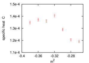
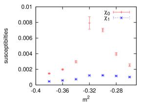
Figure 1: The specific heat $C$ (on the left) and the susceptibilities $\chi_{0}$ and $\chi_{1}$ (on the right, defined in eq. (2.19)) for $N=16,$ $R=4$ and $\lambda=0.44$. The location of the maximum of $C$ coincides with the peak in $\chi_{0}$, which provides a consistent result for the critical value $m_{c}^{2}\simeq-0.32\,$.

This agreement between the two criteria gives a reliable determination of $m_{c}^{2}$. Figure 2 shows this consistency in the case $N=12$, $R=8$ for a variety of $\lambda$ values. It also gives an overview of the phase diagram: as $\lambda$ rises, $m_{c}^{2}$ moves to more negative values. This relation is linear to a good approximation, as we are going to discuss in Section 4.

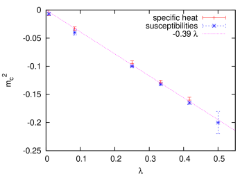
Figure 2: The order/disorder transition line in the phase diagram for $N=12$, $R=8$. The transition is identified consistently from two criteria. This figure shows the regime of weak coupling, where $m^{2}<m_{c}^{2}$ implies a uniform order.

For fixed values of $N$ and $R\,$, the $(\lambda,m^{2})$-plane contains a triple point, which we denote as $(\lambda_{T},m_{T}^{2})$. It separates the regimes of weak coupling, $\lambda<\lambda_{T}$, and of moderate or strong coupling, $\lambda\mathop{\raise 1.29167pt\hbox{$>$\kern-7.5pt\raise-4.73611pt\hbox{$\sim$}}}\lambda_{T}$ or $\lambda\gg\lambda_{T}$.

A typical example for the behaviour of the order parameters at weak coupling is shown in Figure 3. For sufficiently negative $m^{2}$ the order parameter $\langle\varphi_{0}\rangle$ rises drastically. The peaks in $\chi_{0}$ and in the specific heat allow for a more accurate evaluation of $m_{c}^{2}=-0.12(2)$. Further insight into this phase transition is gained by splitting the internal energy $U$ (in eq. (2.20)) into contributions due to the different terms in the action (2.6),

$U_{1}=\frac{2\pi R^{2}}{N}\langle{\rm Tr}[\sum_{t}(\Phi_{t+1}-\Phi_{t})^{2}]\rangle$	: spatial kinetic contribution
$U_{2}=\frac{2\pi}{N}\langle{\rm Tr}[\sum_{t}(\Phi_{t}\hat{\cal L}^{2}\Phi_{t})]\rangle$	: temporal kinetic contribution
$U_{3}=\frac{2\pi R^{2}m^{2}}{N}\langle{\rm Tr}[\sum_{t}\Phi_{t}^{2}]\rangle$	: contribution due to the mass term
$U_{4}=\frac{\pi R^{2}\lambda}{N}\langle{\rm Tr}[\sum_{t}\Phi_{t}^{4}]\rangle$	: contribution due to the self-interaction.

They fulfil the identities

$$U_{1}+U_{2}+U_{3}+U_{4}=U\ ,\quad 2(U_{1}+U_{2}+U_{3}+2U_{4})=1\ ,$$ (3.1)

(the latter is obtained from a variational argument). In our setting the total internal energy $U$ is identical to the entropy. The last plot in Figure 3 illustrates that it deviates from a constant as $m^{2}$ is decreased below $m_{c}^{2}$. Moreover we see that $U_{3}$ and $U_{4}$ drift away from zero at this transition: the quadratic term becomes negative and the quartic term positive, which is just the situation that triggers spontaneous symmetry breaking with uniform ground states.

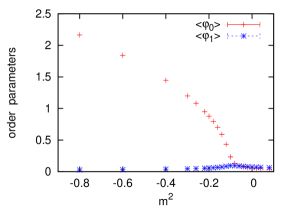
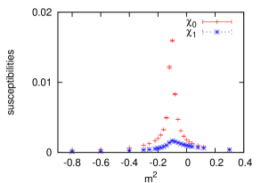
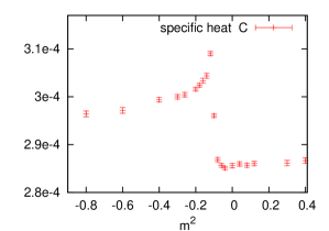
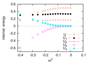
Figure 3: Simulation results for the determination of $m_{c}^{2}$ at $N=12$, $R=4$, $\lambda=0.17$. On top we show the order parameters according to specification (2.18) (on the left) and the corresponding susceptibilities (on the right). We observe a transition between disorder and uniform order at $m_{c}^{2}=-0.12(2)$.
Below: the specific heat (on the left) and different contributions to the internal energy $U=\sum_{i=1}^{4}U_{i}$ (on the right). In the phase of uniform order, the potential terms deviate significantly from zero, so that the mass term $U_{3}$ (the quartic term $U_{4}$) becomes negative (positive). The kinetic contributions $U_{1}$ (spatial) and $U_{2}$ (temporal) remain almost constant — here each dimension contributes approximately the same amount.

Let us proceed to the regime of moderate coupling. Figure 4 shows the order parameters for an example in that regime, along with the susceptibilities. The data reveal a transition between disorder and non-uniform order at $m_{c}^{2}=-0.37(2)$. To provide an overview, we sketch in Figure 5 the complete phase diagram obtained at $N=16$, $R=8$, as a further example.

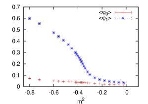
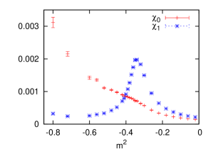
Figure 4: The order parameters and susceptibilities for an example at moderate coupling, $N=12$, $R=8$, $\lambda=1.25$. At $m^{2}\simeq-0.37$ we observe a transition between disorder and non-uniform order.

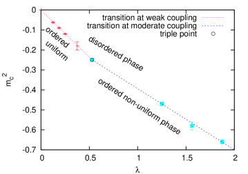
Figure 5: Overview of the phase diagram at $N=16$ and $R=8$.

4 The scaling of the phase transitions

In this section we analyse the scaling of the observed phase transition lines — and in particular their intersection in the triple point — with respect to $N$ and $R$. We proceed by considering separately the boundaries of the disordered phase with the two ordered phases.

4.1 Transition between the disordered and the uniform ordered phase

We first return to the fixed size $N=12$, $R=8$. Figure 2 shows the measured disorder/uniform order transition line,

$$m_{c}^{2}=-0.39(2)\lambda\ .$$ (4.1)

Probing also other sizes — by varying $N$ and $R$ separately — we observed linear relations again, so we were guided to the ansatz

$$m_{c}^{2}=f(N,R)\,\lambda\ ,\qquad f(N,R)\propto N^{\delta_{N}}R^{\delta_{R}}\ .$$ (4.2)

In the last expression we anticipate that the function $f(N,R)$ can be parameterised successfully in a monomial form. To illustrate this, we first fix again $R=8$ but vary $N$ in the range $8\dots 33$. Figures 6 and 7 (on the left) show that we obtain excellent fits with the exponent $\delta_{N}\simeq 0.64$ at $R=4\dots 16$. By including similar plots for $R=2$ and $32$ we extract

$$\delta_{N}=0.64(3)\ .$$ (4.3)

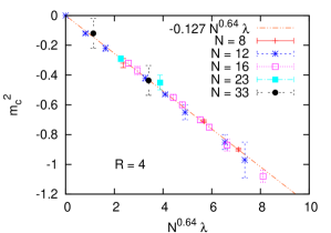
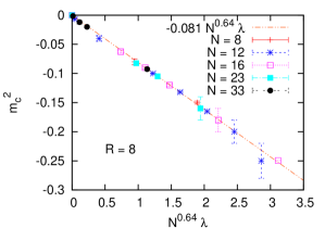
Figure 6: The phase transition disorder/uniform order at $N=8\dots 33$ for $R=4$ (on the left), and for $R=8$ (on the right) . We observe consistency with the exponent $\delta_{N}\simeq 0.64$ given in eq. (4.3).

Subsequently we explore the dependence of $f(N,R)$ on $R$, and we find again agreement with the monomial ansatz (4.2). Moreover, it turns out that the function $f$ essentially just depends on the ratio $N/R$. The exponent $\delta_{R}$ and the coefficient are determined from the fit in Figure 7 (on the right), and we arrive at

$$m_{c}^{2}=-0.31(1)\frac{N^{0.64(3)}}{R^{0.64(1)}}\,\lambda\ ,\qquad(\lambda\leq\lambda_{T})\ .$$ (4.4)

We add that the quality of the corresponding fits is very good as long as $3/8\mathop{\raise 1.29167pt\hbox{$<$\kern-7.5pt\raise-4.73611pt\hbox{$\sim$}}}N/R\mathop{\raise 1.29167pt\hbox{$<$\kern-7.5pt\raise-4.73611pt\hbox{$\sim$}}}8$. If the ratio $N/R$ leaves this interval on either side, the data request a more general function $f(N,R)$ — beyond the monomial form — though the ansatz for $m_{c}^{2}$ as a linear function of $\lambda$ remains applicable over a wider range.

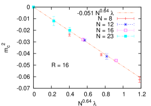
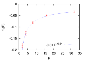
Figure 7: On the left: the transitions disorder/uniform order at $R=16$ for a variety of $N$ values. On the right: the fit for the function $f_{1}(R):=f(N,R)N^{-0.64}$, which yields eq. (4.4) for the phase transitions at weak coupling.

4.2 Transition between the disordered and the non-uniform ordered phase

Figure 8 (on the left) shows the extension of Figure 2 to much stronger couplings $\lambda$. The critical values $m_{c}^{2}$ now mark the transition between disorder and non-uniform order. Over this range of $\lambda$ the phase transition line is curved. However, at this stage we concentrate on the vicinity of the triple point, which is around $(\lambda_{T},m_{T}^{2})\simeq(0.60,\,-0.23)$ in this diagram. Up to $\lambda\approx 3$ a linear fit for $m_{c}^{2}$ is again very precise, but it now requires an additive constant, $m_{c}^{2}=-0.11(2)-0.22(1)\lambda\,$.

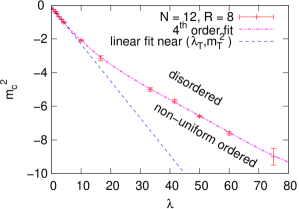
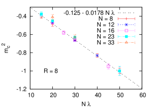
Figure 8: The transition disorder/non-uniform order at $R=8$ and $N=12$ (on the left), and $N=8\dots 33$ (on the right).

We extend also this consideration to $N=8\dots 33$, see Figure 8 on the right. A global fit implies the generalised form

$$m_{c}^{2}=-0.125(25)-0.0178(10)N\lambda\ .$$ (4.5)

In analogy to Subsection 4.1 we repeated this study for $R=2,\,4,\,16$ and $32$; the case $R=16$ is shown as an example in Figure 9 (on the left). Since the choice of $N\lambda$ as the parameter on the $x$-axis works well in all these cases, we are led to the ansatz

$$m_{c}^{2}=-g(R)-h(R)N\lambda\ ,\qquad(\lambda\mathop{\raise 1.29167pt\hbox{$>$\kern-7.5pt\raise-4.73611pt\hbox{$\sim$}}}\lambda_{T})\ .$$ (4.6)

Figure 9 (on the right) shows our fits for the functions $g(R)$ and $h(R)$, which imply

$$g(R)=6.0(15)R^{-1.92(10)}\ ,\quad h(R)=0.082(7)R^{-0.72(4)}\ .$$ (4.7)

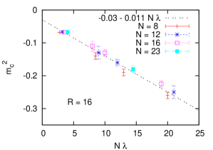
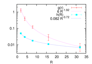
Figure 9: On the left: the transition disorder/non-uniform order in the phase diagram at $R=16$. On the right: the fits for the functions $g(R)$ and $h(R)$, which lead to the form (4.7).

4.3 The triple point

We are now in a position to evaluate the triple point by the intersection of the phase transition lines at low and moderate coupling, given in eq. (4.4), and in eqs. (4.6), (4.7). The intersection point is located at

$$(\lambda_{T},m_{T}^{2})\simeq\frac{\Big{(}19(5)R^{-1.20(11)}N^{-0.64(9)},-5.9(16)R^{-0.56(11)}N^{0.0(1)}\Big{)}}{R^{0.08(4)}-0.26(2)N^{0.36(9)}}\ .$$ (4.8)

We assume Gaussian error propagation, and include a possible error on the power of $N$ in the ansatz (4.6).

This equation parameterises the triple point in the range for $N$ and $R$ that we simulated. However, this formula cannot be extrapolated to large $N$, due to the form of the denominator. A direct investigation of the triple point — and therefore of the phase diagram — in the thermodynamic limit would require simulations at very large $N$. We will come back to this issue in Section 6, where we conjecture the properties of this extrapolation indirectly.

5 Confrontation with related models

Having elaborated the features of the phase diagram, we now compare it to related models, which were also simulated in the recent years, and to reduced matrix models, which have been studied analytically.

5.1 The 2d $\lambda\phi^{4}$ model on a fuzzy sphere

At finite $N$, the phase diagram for the 2d $\lambda\phi^{4}$ model on a fuzzy sphere is qualitatively the same as we found in Section 3. An explicit convergence of our model to the 2d case could be expected in a setting which renders solely the temporal kinetic term negligible. We saw, however, in Figure 3 that the impact of this term remains significant and approximately constant at weak and moderate coupling. This property is generic in our study, hence there is no basis for expecting a reduction to the 2d model on a fuzzy sphere. At large $\lambda$ some reduction sets in, but it is of a different kind, see Subsection 5.3.

5.2 Comparison with a non-commutative torus

Ref. [19] presented a related numerical study of the 3d $\lambda\phi^{4}$ model: also there the Euclidean time was lattice discretised, while the spatial dimensions were treated by non-commutative coordinates. However, a lattice formulation and periodic boundary conditions were assumed for the spatial directions as well, and the non-commutativity tensor $\Theta_{\mu\nu}$ was constant. By means of Morita equivalence [24] the scalar field — first defined on a $N\times N$ lattice in the non-commutative plane — was mapped onto Hermitian $N\times N$ matrices, so the action ultimately simulated was similar to eq. (2.6) (and also the rule (2.21) was the same). The difference is the form of the spatial kinetic term: on the non-commutative plane it was constructed by an adjoint matrix operation which represents a shift by one lattice unit.

The phase diagram at finite $N$ was qualitatively equivalent to the form that we found here. On the torus the non-uniform ordered phase was denoted as “striped phase”, and the stripe formation for the two signs of $\phi_{t}(x_{1},x_{2})$ could indeed be visualised by mapping the matrices back to 2d lattice configurations (at a fixed time site).

Let us proceed to a quantitative comparison. On the torus the boundary of the disordered phase was approximately identified as [19]

$${\rm disorder/uniform~{}:}\quad m_{c}^{2}\simeq-0.80\lambda\qquad\qquad\qquad\qquad$$ (5.1)

$${\rm disorder/non\!\!-\!\!uniform~{}:}\quad m_{c}^{2}\simeq-0.48\lambda-\frac{80}{N^{2}}$$ (5.2)

$${\rm triple~{}point~{}:}\quad (N^{2}\lambda_{T},N^{2}m_{T}^{2})\approx(250,\,-200)\ .\qquad$$ (5.3)

The transition disorder/non-uniform order was only explored up to moderate coupling, $\lambda=O(1)$.

Our corresponding results are given in eqs. (4.4) and (4.6) to (4.8). The transition line (5.1) can be matched if we set $R\simeq 0.23N$, but the triple point still differs strongly. However, in the weak coupling region a link between the two models can hardly be expected, due to the significance of the spatial kinetic term.

We proceed to moderate coupling and look at the requirements for agreement with eq. (5.2). The condition for the function $g(N,R)$ reads $R\simeq 0.26N^{1.04}$, which is close to the above requirement for eq. (5.1). On the other hand, the condition due to the function $h(N,R)$ deviates more from this pattern, in particular in view of the exponent ($R\simeq 0.28N^{1.39}$).

We anticipate at this point that the geometrical picture — to be described in Section 6 — suggests that the non-commutative plane emerges for

$$R\propto N^{\beta}\ ,\quad\beta=1/2\ .$$ (5.4)

Hence the value for $\beta$ obtained at moderate $\lambda$ takes us even further away from the geometrical picture. This may appear somewhat surprising, but it is not paradoxical. For $\lambda/\lambda_{T}=O(1)$ the spatial kinetic term is significant, as the example in Figure 3 shows, so a difference in this term may well displace the phase transition lines.

In addition we saw that our results in Section 4 suffer from finite $N$ artifacts, hence the considerations in this and the previous Subsection have to be interpreted cautiously.

5.3 Reduction to a matrix chain

At strong coupling $\lambda$ the impact of the kinetic terms is reduced. In the extreme case where they are fully negligible, one could imagine a transition to a 1-matrix model of a single Hermitian random matrix $\Phi_{1}$ with the potential $\,4\pi R^{2}\cdot{\rm Tr}\,[\frac{m^{2}}{2}\Phi_{1}^{2}+\frac{\lambda}{4}\Phi_{1}^{4}]\,$. That model has been studied analytically at $m^{2}\geq 0$ [25] and at $m^{2}<0$ with the result [26]

$$m_{c}^{2}=-\frac{N}{R}\sqrt{\frac{\lambda}{\pi}}\ .$$ (5.5)

Consistent numerical data have been reported for the 2d $\lambda\phi^{4}$ model on a fuzzy sphere [8] and on a non-commutative plane [27]. In our simulations we explored values up to $\lambda=O(10^{2}\dots 10^{3})$, but we could not observe the feature of eq. (5.5) [11].

We did find, however, consistency with a partial reduction, which only neglects the spatial kinetic term; this is opposite to the scenario commented on in Subsection 5.1. In our formulation (2.6) this means that the double-commutators $[{\cal L}_{i},[{\cal L}_{i},\Phi_{t}]]$ are negligible. This behaviour is exactly confirmed by Figure 10. Thus we obtain a matrix chain (analogous to a spin chain), consisting of Hermitian matrices with a quartic potential, which are linked by a discrete second derivative. In the large $N$ limit Ref. [26] derived the critical line

$$m_{c}^{2}=-\Big{(}\frac{3N^{2}}{16R^{2}}\,\lambda\Big{)}^{2/3}\ .$$ (5.6)

This formula corresponds to the one-cut vs. two-cut transition in the eigenvalue distribution of random matrices. This transition plays an essential rôle; it must show up at least for sufficiently large $\lambda$. In addition it is of importance down to the triple point, where it merges with the transition to the uniform order. But as the coupling is lowered, the fuzzy kinetic term distorts the form (5.6) for this transition line. It eventually terminates at the triple point — a feature not present in the matrix chain.

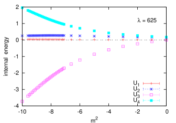
Figure 10: The different contributions to the internal energy at $N=8$, $R=16$ and $\lambda=625$. The temporal kinetic contribution $U_{2}$ now clearly dominates over the spatial kinetic contribution $U_{1}$, in contrast to the weak coupling behaviour shown in the last plot of Figure 3. This is fully consistent with the observed reduction in the spatial directions only, which leads to the matrix chain behaviour described in Ref. [26].

Figure 11 shows two examples where the behaviour of eq. (5.6) is matched accurately, up to a modification in the coefficient.

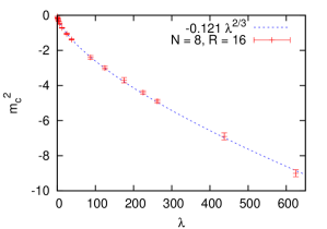
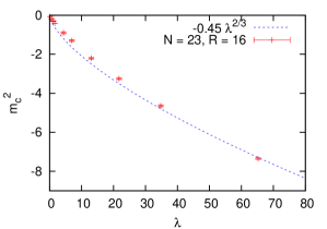
Figure 11: The phase transition at strong coupling $\lambda$ for $N=8$, $R=16$ (on the left), and for $N=23$, $R=16$ (on the right). In both cases we observe a broad window of agreement with the matrix chain formula (5.6).

We take a closer look at the first case, $N=8$, $R=16$, where the precise agreement with the exponent in eq. (5.6) is amazing because of the relatively small matrices. We further fix $\lambda=625$ and we show in Figure 12 the specific heat and the order parameters. The former confirms the critical parameter $m_{c}^{2}=-9.0(5)$ which appears in Figure 11. The order parameters demonstrate that we deal with a transition between disorder and non-uniform order, where the latter corresponds now to the condensation of higher modes, $\ell>1$ (unlike the examples in Subsection 4.2).

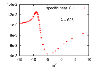
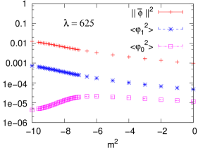
Figure 12: The specific heat (on the left) and the order parameters (on the right) at $N=8$, $R=16$ and $\lambda=625$. We confirm the critical value $m_{c}^{2}=-9.0(5)$ at the transition between disorder and a non-uniform order (cf. Figure 11 on the left). The plot on the right demonstrates that it corresponds to a higher mode condensation, i.e. to a non-uniform order with a complicated pattern.

This type of model (matrix quantum mechanics) has applications in various branches of physics. For instance QCD with $N_{f}$ light quarks flavours in a small box but an elongated time direction (the so-called “$\delta$-regime”) can be treated effectively by quantum mechanics of $SU(N_{f})$ matrices [28]. The very same technique can also be applied in solid state physics [29].

Our case of Hermitian matrices attracted attention in string theory since the early nineties [30, 31]. In that framework it represents the $c=1$–model, which describes random surfaces moving in one dimensions. At a finite time periodicity $T$ there is a vortices-driven Kosterlitz-Thouless phase transition to the $c=0$–model [30, 32]. Possible links to QCD₂, to 2d black holes and to topological field theory were studied intensively [33]. This model continues to attract interest, see Refs. [34] for recent examples.

An overview of the different reduction scenarios is added in Table 2.

spatial	temporal	setting	status
kin. term	kin. term
		2d model on	numerical studies [8]
large	small	a fuzzy sphere	not attained here
		matrix chain	analytical studies [25, 26]
small	large	or c=1-model	reproduced here at large $\lambda$
		total reduction	analytical study [26]
small	small	1-matrix model	not attained here

Table 2: An overview of the conceivable reductions of our system — due to the negligibility of kinetic terms — and their status in the literature and in this work.

6 A conjecture about the large $N$ limit

In this section we discuss the extrapolation of the phase diagram to large $N$ (which represents the thermodynamic limit) and to large $R$ (the transition of the spatial part to a plane). In addition our rule (2.21) connects the large $N$ limit with the thermodynamic limit in the temporal direction.

We first consider the geometry of the sphere under these limits. As we remove the cutoff $N$, the coordinates (2.3) describe different 2d spaces, depending on the simultaneous treatment of the radius $R$:

• The limit $N\to\infty$ at $R=const.$ leads to a sharp sphere.

• If the radius grows slowly, $R\propto N^{\beta}$, $0<\beta<1/2$, we end up with a sharp plane in the large $N$ limit.

• If we take instead $N\propto R^{2}\to\infty$ we obtain a non-commutative plane with a constant non-commutativity tensor $\Theta_{\mu\nu}={\rm i}\,\theta\,\epsilon_{\mu\nu}$ (where $\mu,\,\nu\in\{1,2\}$). This can be seen for instance in the plane which emerges around the point $(0,0,1)$,

  $$[X_{1},X_{2}]\simeq{\rm i}\frac{2R^{2}}{\sqrt{N^{2}-1}}\,\frac{X_{3}}{R}\quad\Rightarrow\quad\theta=\frac{2R^{2}}{N}\ .$$ (6.1)

The scaling behaviour of a field theory on this space, and in particular its phase diagram, still has to be investigated. For the parameter range simulated, this was carried out in Section 4. We now address the issue of the large $N$ extrapolation, which was postponed in Section 4. For the disorder/non-uniform order transition, we found agreement with the eqs. (4.6) and (4.7) at moderate $\lambda$, and with eq. (5.6) at strong $\lambda$ (up to a modest modification of the coefficient). In either case $\lambda$ only occurs in a product with a positive power of $N$ ($1$ resp. $4/3$). This is consistent with the suppression of field fluctuations at large $N$ or large $\lambda$. Based on this property, we conjecture that exploring the large $N$ behaviour could be equivalent to the case of large $\lambda$ at the values of $N$ in our study.

This means that we now refer to eq. (5.6) to determine the triple point. The behaviour

$$m_{c}^{2}=-c(N/R)^{4/3}\lambda^{2/3}\qquad(c=const.)$$ (6.2)

is compatible with our data. For instance at $R=16$ we obtained $m_{c}^{2}\lambda^{-2/3}\simeq-0.121$ at $N=8$, and $-0.31$ at $N=16$ (see Figures 11 and 13), which matches very well the behaviour $m_{c}^{2}\propto N^{4/3}$. Also the dependence of the radius follows eq. (6.2): for example the results at $N=8$ and $R=8$ vs. $R=16$ (in Figures 11 and 13) agree very well with the relation $m_{c}^{2}\propto R^{-4/3}$.

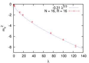
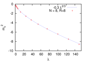
Figure 13: The phase transition at strong coupling $\lambda$ for $N=16$, $R=16$ (on the left), and for $N=8$, $R=8$ (on the right). As in Figure 11 we find agreement with the matrix chain prediction $m_{c}^{2}\propto\lambda^{2/3}$. In addition, comparison to the result for $N=8$, $R=16$ in Figure 11 supports the full proportionality relation (6.2).

Considering many fits of that kind [11] we found that both exponents and the coefficients $c$ in eq. (6.2) fluctuate within about $10\%$ around the theortical values of eq. (5.6), which were derived for the matrix chain at large $N$ [26].

The intersection of this curve with the disorder/uniform order transition line (4.4) yields

$$\lambda_{T}\propto\frac{N^{2.1(2)}}{R^{2.1(1)}}\ .$$ (6.3)

In the framework of this conjecture, we obtain the following scenarios for the limit $N\to\infty$:

• Limits with $N\to\infty$, $N/R\to\infty$ remove the phase of non-uniform order. Then the ordered regime only consists of the uniform phase, which is separated by an Ising transition from the disordered phase. This limit corresponds to a commutative model. It includes in particular the case of a sharp sphere ($R=const.$). In contrast to the tree-level expectation, this class of limits also captures the case $N\propto R^{2}$, which geometrically leads to a non-commutative plane.

• If the limits $N,\,R\to\infty$ are taken such that the ratio $N/R$ remains finite, the triple point stabilises and the phase diagram keeps qualitatively the form that we observed at finite $N$; all three phases persist.

• Limits with $N\to\infty$, $N/R\to 0$ remove the phase of uniform order. Now the ordered regime consists solely of the non-uniform phase. This scenario is obtained for a rapidly expanding sphere. Here the non-commutativity dominates the thermodynamic limit.

The transition lines that we identified at small and at moderate coupling in Section 4 do not scale simultaneously for for any fixed choice of the axes of the phase diagram, as the forms (4.4) and (4.6) show. On the other hand, the large $N$ behaviour (as conjectured in this section) overcomes this problem: if the triple point moves to $0$ or $\infty$, only one transition line survives. In the case $R\propto N$, which stabilises a finite triple point, the axes $(\lambda,m^{2})$ apply to both transition lines, without the necessity of rescaling.

7 Conclusions

We presented a numerical study of the phase diagram in the 3d $\lambda\phi^{4}$ model, where the spatial part is regularised on a fuzzy sphere, while the Euclidean time is lattice discretised. On the regularised level, we identified three phases based on the order parameters $\varphi_{\ell}$ in eq. (2.2), the corresponding susceptibilities and the specific heat. At fixed $\lambda$ there is a critical parameter $m_{c}^{2}<0$ : for $m^{2}>m_{c}^{2}$ ($m^{2}<m_{c}^{2}$) the system is disordered (ordered). The transition to $m^{2}<m_{c}^{2}$ leads to a uniform order at small $\lambda$, and to a non-uniform order at moderate or large $\lambda$.

The boundary between these two scenarios corresponds to the triple point, which we denoted as $(\lambda_{T},m_{T}^{2})$. The transition disorder/uniform order (at $\lambda<\lambda_{T}$) is analogous to a spontaneous magnetisation and its critical line is parameterised by eq. (4.4).

The non-uniform ordered phase emerges as a consequence of the non-locality in the fuzzy sphere regularisation. That phase does not occur in a pure lattice regularisation. It corresponds to a spontaneously broken rotation symmetry. At moderate coupling strength, $\lambda\mathop{\raise 1.29167pt\hbox{$>$\kern-7.5pt\raise-4.73611pt\hbox{$\sim$}}}\lambda_{T}$, the critical line is described by eqs. (4.6) and (4.7). From its intersection with the curve (4.4) we infer the location of the triple point given in eq. (4.8). This formula captures a large amount of data that we collected, but it cannot be extrapolated to the limit $N\to\infty$.

Next we discussed the relation between the system studied here and some models investigated in the literature, which have qualitatively similar phase diagrams at finite $N$. We found, however, significant differences from the 2d $\lambda\phi^{4}$ model an a fuzzy sphere [8]. As for the 3d $\lambda\phi^{4}$ model on a non-commutative torus [19] the vicinity of the triple point can be matched rather roughly for a suitable relation between $N$ and $R$.

At large $\lambda$, we observed consistency with the reduction to a matrix chain model, which had been solved in the large $N$ limit [26]. In particular our data match precisely the predicted relation $m_{c}^{2}\propto(N^{2}\lambda/R^{2})^{2/3}$. That model is known as the $c=1$–model in string theory [30, 31, 32, 33, 34], which we have therefore captured non-perturbatively.

We then conjectured that large $N$ values may be equivalent to large $\lambda$ couplings at moderate $N$, since $N$ and $\lambda$ tend to appear only as products in the formulae for the phase transition lines. This conjecture leads to different limits depending on the exponent $\beta$ in the relation $R\propto N^{\beta}$. For $\beta<1$ we obtain a commutative limit, with an Ising-type transition between disorder and uniform order. On the other hand, a rapidly expanding sphere ($\beta>1$) leads to a dominance of the non-uniform phase. That feature is a characteristic for a non-commutative theory, where UV/IR mixing gives rise to an ordering due to the condensation of a non-zero mode [16, 17, 18, 19].

It remains an open question to verify the conjectured limits by direct inspection of the triple point at very large system sizes $N$. For instance, at $R=const.$ one should verify the properties of the fuzzy sphere at larger $N$. In the light of gravity-induced non-commutativity on the Planck scale [35], a relation to quantum effects in a black hole might be conceivable (see e.g. Refs. [32, 36] for this line of thought).

According to our conjecture, the distinction between the scenarios of a commutative and a non-commutative limit is not located at the point where it is expected on purely geometrical grounds ($\beta=1/2$). Furthermore, it does not coincide with the picture suggested by a perturbative calculation to two loops [20]. In that picture the commutative continuum limit could not be retrieved at all because of the UV/IR mixing [20].

A general lesson is that non-locality — once it is introduced — can cause surprises in the extrapolations on the non-perturbative level. This observation may serve as a warning also for the use of non-local actions in lattice simulations, such as rooted staggered fermions (cf. footnote 4) or overlap fermions [37] at strong gauge coupling. On the other hand, such surprises may provide insight into other universality classes of interest, as we have seen. However, using the fuzzy sphere as a regularisation scheme in quantum field theory is not straightforward and its application requires a careful investigation of the phase diagram.

Appendix A Technical aspects of the simulation

Our simulations were based on the Metropolis algorithm. In each step we updated only one pair of conjugate matrix elements, $(\Phi_{t})_{ij}=(\Phi_{t})_{ji}^{*}\,$. A detailed comparison in technically similar simulations revealed that this is far more efficient than updating complete matrices $\Phi_{t}$ [19]. It proved useful to propose independent changes of the real and the imaginary part of $(\Phi_{t})_{ij}$ with absolute values below $N\sqrt{m^{2}/\lambda}$ (and flat probability distribution); this led to acceptance rates typically around $1/2$. One sweep applies this step successively to all independent elements in a configuration $\Phi$.

We were often confronted with several local minima of the action. In many cases these minima were too pronounced for a tunnelling to occur even in histories involving $O(10^{7})$ sweeps. This property obviously obstructs the direct measurement of observables. As a first remedy we performed a number of runs with independent hot starts. At the end we summed up the statistics collected in each run after thermalisation (which we are going to comment on below). The histories in all runs had the same length of $O(10^{6})$ sweeps. This improves the situation, but the number of runs was still too small (typically $O(10)$) to sample the vicinities of the different minima reliably.

Therefore we extended the algorithm as follows. We stored the end configuration of each run as $\Phi_{\rm end}$. The subsequent run takes a new hot start, but after thermalisation the current configuration may be replaced by $\Phi_{\rm end}$ through a Metropolis accept/reject step, before the history continues. We denote this method as adaptive Metropolis algorithm. In fact it improves the statistically correct inclusion of the vicinities around various minima, and it leads to stable and sensible measurements, as the examples in Figure 14 illustrate. The impact of higher local minima tends to be overestimated by fully independent runs. The additional Metropolis step helps to overcome this artifact; in particular the global minimum now receives the suitable weight. Figure 15 (on the left) shows an example for this effect.

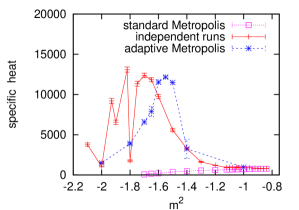
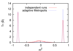
Figure 14: An illustration of the progress due to the adaptive Metropolis algorithm. The parameters in these examples are $N=12,$ $R=4$, $\lambda=1.83$. On the left we show the specific heat $C$; for adaptive Metropolis only the peak is clearly observed at the critical value $m_{c}^{2}$. The plot on the right is a histogram for ${\rm Tr}(\bar{\Phi})$ at $m^{2}=-1.7$, i.e. in the phase of uniform order. The two peaks approximate the expected symmetric form well with adaptive Metropolis, but not with the same number of independent runs.

In principle the variety of metastable vacua can be regarded as a severe thermalisation problem. However, since it is taken care of by the adaptive Metropolis step, we reduce our notion of thermalisation to the Monte Carlo time in each run until the observables stabilise over a long period at the value that corresponds to the chosen minimum. In this respect, about 2000 sweeps were sufficient to thermalise quantities like the action and our order parameters (introduced in Section 2).

While this thermalisation is harmless, a technical problem could occur due to a large number of local minima, in particular at $\lambda\gg\lambda_{T}$. For a simplified consideration we assume the kinetic terms to be negligible (although we saw in Subsection 5.3 that this complete reduction is not really achieved). Then the matrices $\Phi_{t}$ are independent and — in a minimum of the potential — each one can be transformed to a diagonal form with elements $\pm\sqrt{|m^{2}|/(N\lambda)}$. With all sign combinations the term $\bar{c}_{00}=\sqrt{4\pi}\cdot{\rm Tr}(\bar{\Phi})/N^{2}$ can take $N^{2}+1$ values, which is a considerable number for the system sizes that we studied. However, for independent random signs the values near zero dominate, whereas the probabilities for minima with large $\varphi_{0}=|\bar{c}_{00}|$ are suppressed. For instance Figure 15 (on the right) shows a histogram for $\bar{c}_{00}$ at $N=12\,$; only $5$ peaks (corresponding to the $5$ dominant minima) are visible.

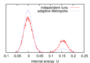
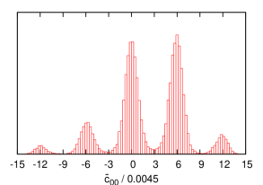
Figure 15: Histograms for two quantities, which are sensitive to the variety of action minima. On the left: the internal energy $U$ measured at $N=12$, $R=4$, $\lambda=1.83$, $m^{2}=-1.7$. On the right: $\bar{c}_{00}$ (see eqs. (2.14), (2.15)) measured at $N=12$, $R=16$, $\lambda=0.75$, $m^{2}=-0.3$. $\bar{c}_{00}$ is shown in units of $2\sqrt{\pi|m^{2}|/(N^{5/2}\lambda)}\simeq 0.0045$ so that the peaks are located at integer values, in agreement with our prediction.

The statistical errors were evaluated independently with the binning and the jackknife method on one hand (we probed various bin sizes), and with the Madras-Sokal method [40] on the other hand. The latter amplifies the standard error by a factor which takes the autocorrelation into account. We generally display the largest (and therefore safest) error bar obtained by these methods.

Acknowledgements   We are indebted to Frank Hofheinz for providing us with a highly optimised parallel code which was applied in this project. We also thank him, as well as Aiyalam Balachandran, Brian Dolan, Fernando Garcia Flores, Giorgio Immirzi, Xavier Martin, Jun Nishimura, Marco Panero, Peter Prešnajder and Jan Volkholz for helpful discussions. J.M. was supported in part by the Secretaría de Investigación y de Posgrado (SIP), and D.O’C. by MTRN-CT-2006-031962. The simulations were performed on PC clusters at DIAS in Dublin and at the Humboldt-Universität zu Berlin.

References

- [1] C.G. Bollini and J.J. Giambiagi, Nuovo Cim. B 12 (1972) 20; Phys. Lett. B 40 (1972) 566. G. ’t Hooft and M. Veltman, Nucl. Phys. B 44 (1972) 189.
- [2] I. Montvay and G. Münster, “Quantum fields on a lattice”, Cambridge University Press (Cambridge UK, 1994).
- [3] G.G. Batrouni, G.R. Katz, A.S. Kronfeld, G.P. Lepage, B. Svetitsky and K.G. Wilson, Phys. Rev. D 32 (1985) 2736.
- [4] A. Connes, “Noncommutative Geometry”, Academic Press (San Diego, 1994).
- [5] H.S. Snyder, Phys. Rev. 71 (1947) 38.
-
[6]
J. Madore, Class. and Quant. Grav. 9 (1992) 69.
H. Grosse, C. Klimčík and P. Prešnajder,
Int. J. Mod. Phys. 35 (1996) 231; Commun. Math. Phys. 180 (1996) 429.
Ideas in this direction were expressed earlier in: F.A. Berezin, Commun. Math. Phys. 40 (1975) 153. J. Hoppe, “Quantum Theory of Massless Relativistic Surfaces”, Ph.D. Thesis, MIT (Cambrdige MA, 1982). - [7] D.A. Varshalovich, A.N. Moskalev and V.K. Khersonky, “Quantum Theory of Angular Momentum”, World Scientific (Singapore, 1998).
- [8] X. Martin, JHEP 0404 (2004) 077. F. Garcia Flores, D. O’Connor and X. Martin, PoS(LAT2005)262. M. Panero, SIGMA 2 (2006) 081; JHEP 0705 (2007) 082. C.R. Das, S. Digal and T.R. Govindarajan, arXiv:0706.0695 [hep-th].
- [9] D. O’Connor and B. Ydri, JHEP 0611 (2006) 016. R. Delgadillo-Blando, D. O’Connor and B. Ydri, arXiv:0712.3011 [hep-th].
- [10] J. Medina, W. Bietenholz, F. Hofheinz and D. O’Connor, PoS(LAT2005)263.
- [11] J. Medina, “Fuzzy Scalar Field Theories: Numerical and Analytical Investigations”, Ph.D. Thesis, CINVESTAV (México D.F., 2006).
- [12] H. Grosse, C. Klimčík and P. Prešnajder, Commun. Math. Phys. 185 (1997) 155. H. Grosse and G. Reiter, J. Geom. Phys. 28 (1998) 349. C. Klimčík, Commun. Math. Phys. 206 (1999) 567. A.P. Balachandran, S. Kürkçüoǧlu and E. Rojas, JHEP 0207 (2002) 056. A.P. Balachandran, A. Pinzul and B. Qureshi, JHEP 0512 (2005) 002. A.P. Balachandran, S. Kürkçüoǧlu and S. Vaidya, hep-th/0511114. B. Ydri, arXiv:0708.3065 [hep-th]; Mod. Phys. Lett. A 22 (2007) 2565. T. Azuma, S. Bal and J. Nishimura, arXiv:0712.0646 [hep-th].
- [13] K.N. Anagnostopoulos, T. Azuma, K. Nagao and J. Nishimura, JHEP 0509 (2005) 046. J. Volkholz and W. Bietenholz, PoS(LAT07)283.
-
[14]
H. Grosse and P. Prešnajder,
Lett. Math. Phys. 33 (1995) 171.
A.P. Balachandran and G. Immirzi, Phys. Rev. D 68 (2003) 065023. -
[15]
M. Creutz, arXiv:0708.1295 [hep-lat].
A. Kronfeld, arXiv:0711.0699 [hep-lat]. - [16] S.S. Gubser and S.L. Sondhi, Nucl. Phys. B 605 (2001) 395.
- [17] G.-H. Chen and Y.-S. Wu, Nucl. Phys. B 622 (2002) 189.
- [18] P. Castorina and D. Zappalà, Phys. Rev. D 68 (2003) 065008.
- [19] W. Bietenholz, F. Hofheinz and J. Nishimura, Acta Phys. Pol. B 34 (2003) 4711; JHEP 06 (2004) 042. F. Hofheinz, “Field theory on a non-commutative plane: a non-perturbative study”, Ph.D. Thesis, Humboldt-Universität (Berlin, 2003), published in Fortsch. Phys. 52 (2004) 391.
- [20] R. Delgadillo-Blando, “Teoría en el espacio tiempo y su límite continuo”, M.Sc. Thesis, CINVESTAV (México D.F., 2002). B.P. Dolan, D. O’Connor and P. Prešnajder, JHEP 03 (2002) 013.
-
[21]
H. Steinacker, JHEP 0503 (2005) 075.
D. O’Connor and C. Sämann, JHEP 0708 (2007) 066. - [22] J. Ambjørn and S. Catterall, Phys. Lett. B 549 (2002) 253.
- [23] P. Castorina and D. Zappalà, arXiv:0711.2659 [hep-th].
- [24] J. Ambjørn, Y.M. Makeenko, J. Nishimura and R.J. Szabo, JHEP 9911 (1999) 029; Phys. Lett. B 480 (2000) 399; JHEP 0005 (2000) 023.
- [25] E. Brezin, C. Itzykson, G. Parisi and J.B. Zuber, Commun. Math. Phys. 59 (1978) 35. D. Bessis, C. Itzykson and J.B. Zuber, Adv. Appl. Math. 1 (1980) 109.
- [26] Y. Shimamune, Phys. Lett. 108 B (1982) 407.
- [27] J. Volkholz, “Nonperturbative Studies of Quantum Field Theories on Noncommutative Spaces”, Ph.D. Thesis, Humboldt-Universität (Berlin, 2007).
- [28] H. Leutwyler, Phys. Lett. B 189 (1987) 197.
- [29] P. Hasenfratz and F. Niedermayer, Z. Phys. D 92 (1993) 91.
- [30] D.J. Gross and I.R. Klebanov, Nucl. Phys. B 344 (1990) 475.
- [31] D.J. Gross and I.R. Klebanov, Nucl. Phys. B 354 (1991) 459; Nucl. Phys. B 359 (1991) 3. D.J. Gross, I.R. Klebanov and M.J. Newman, Nucl. Phys. B 350 (1991) 621.
- [32] A. Mukherjee and S. Mukhi, JHEP 0607 (2006) 017.
- [33] An early review is included in: P.H. Ginsparg and G.W. Moore, hep-th/9304011.
- [34] S. Alexandrov, JHEP 0405 (2004) 025. J.L. Karczmarek and A. Strominger, JHEP 0405 (2004) 062. J.M. Maldacena, Int. J. Geom. Meth. Mod. Phys. 3 (2006) 1. C. Gómez and R. Hernández, Phys. Lett. B 644 (2007) 375.
- [35] S. Doplicher, K. Fredenhagen and J.E. Roberts, Commun. Math. Phys. 172 (1995) 187.
- [36] B.P. Dolan, JHEP 0502 (2005) 008. H. Garcia-Compean and C. Soto-Campos, Phys. Rev. D 74 (2006) 104028.
- [37] H. Neuberger, Phys. Lett. B 417 (1998) 141.
- [38] P. Hernández, K. Jansen and M. Lüscher, Nucl. Phys. B 552 (1999) 363.
- [39] W. Bietenholz, Eur. Phys. J. C 6 (1999) 537; Nucl. Phys. B 644 (2002) 223. W. Bietenholz and I. Hip, Nucl. Phys. B 570 (2000) 423. T.A. DeGrand, Phys. Rev. D 63 (2001) 034503. P. Hasenfratz, S. Hauswirth, T. Jörg, F. Niedermayer and K. Holland, Nucl. Phys. B 643 (2002) 280. W. Bietenholz and S. Shcheredin, Nucl. Phys. B 754 (2006) 17.
- [40] N. Madras and A.D. Sokal, J. Statist. Phys. 50 (1988) 109.