Design of three dimensional isotropic microstructures for maximized stiffness and conductivity

Abstract

The level–set method of topology optimization is used to design isotropic two–phase periodic multifunctional composites in three dimensions. One phase is stiff and insulating whereas the other is conductive and mechanically compliant. The optimization objective is to maximize a linear combination of the effective bulk modulus and conductivity of the composite. Composites with the Schwartz primitive and diamond minimal surfaces as the phase interface have been shown to have maximal bulk modulus and conductivity. Since these composites are not elastically isotropic their stiffness under uniaxial loading varies with the direction of the load. An isotropic composite is presented with similar conductivity which is at least 23% stiffer under uniaxial loading than the Schwartz structures when loaded uniaxially along their weakest direction. Other new near–optimal isotropic composites are presented, proving the capablities of the level–set method for microstructure design.

, ,

1 Introduction

The design of multifunctional materials is a growing field. Torquato et al. (2002, 2003) considered the simultaneous transport of heat and electricity in three dimensional biphasic composites where one phase was more thermally conducting and less electrically conducting than the other. The structures were required to be isotropic by imposing threefold reflection symmetry. When both thermal and electrical conductivity were maximized the resultant composite resembled a Schwartz primitive (P) structure. The optimality of the Schwartz P structure and also of the Schwartz D structure for maximizing both conductivity properties was shown numerically via finite element calculations and using rigorous cross–property bounds. Following this work, Torquato and Donev (2004) used finite element calculations to show the optimality of Schwartz P and D structures for maximum bulk modulus and conductivity for any ill–ordered phase properties (one phase has a larger conductivity but a smaller bulk modulus and shear modulus than the other phase). These publications demonstrated that structures derived from Schwartz P and D minimal surfaces are important multifunctional composites.

Guest and Prévost (2006) designed microstructures to maximize bulk modulus and fluid permeability. They demanded cubic elastic symmetry and isotropic flow symmetry and used the solid isotropic material with penalization (SIMP, Bendsøe, 1989; Bendsøe and Kikuchi, 1988) implementation of topology optimization. Stokes’ flow conditions were assumed to calculate fluid permeability and optimized structures were presented for different coefficients in the optimization objective. For particular coefficients in the multiobjective design problem they obtained structures very similar to the Schwartz P structure, consistent with the results of Torquato and Donev (2004).

The recent paper of de Kruijf et al. (2007) considered optimal structures with maximum stiffness and minimum resistance to heat dissipation and the design of two dimensional composite materials with maximal effective thermal conductivity and bulk modulus. The two phases for the design problem were ill–ordered. The microstructures were required to be isotropic with respect to conductivity but only square–symmetric with respect to elasticity. The SIMP topology optimization algorithm was used.

In this paper, two-phase isotropic three dimensional periodic composites are designed using topology optimization to have maximal bulk modulus and conductivity. The two isotropic phases for the microstructure design problem are ill–ordered infinite–contrast materials: one of the phases has finite stiffness but zero conductivity, whereas the other phase has finite conductivity and zero stiffness. The result is competition between the phases. In particular, for the composite to have nonzero stiffness and nonzero conductivity both phases need to be connected.

Our study is motivated by a desire to design maximally stiff, electrically conducting and isotropic cermets (composites of ceramic and metal), and optimally stiff, porous and isotropic bone implants. In the former situation, the ceramic has high stiffness but low conductivity, whereas the metal has comparatively low stiffness and high electrical conductivity. For implants, the implant material (titanium, for example) has high stiffness but is impenetrable to bone in-growth, whereas the pore space has zero stiffness and allows bone in-growth. Here, the effective conductivity of the pore space is used to model the ease of bone in-growth into the implant. In reality, both scenarios will also involve manufacturing constraints, we deal with the simplest microstructure design problem and such constraints are left for future work. The calculation of electrical conductivity, thermal conductivity, dielectric constant, magnetic permeability and diffusion coefficient are all mathematically equivalent, thus our results can also be applied to those cases. As well as having practical application, the objective function we consider is convenient from a theoretical viewpoint due to the cross–property bounds derived by Gibiansky and Torquato (1996).

The requirement of isotropy with respect to elasticity has not been seen in previous multifunctional composite design work, but can be an important criteria when the directions along which loads will be applied is unknown. In this case it is the strength of the weakest direction which is critical. In particular, we highlight the anisotropic stiffness properties and weak directions of the Schwartz P and D structures to justify the isotropy constraint. As already noted, these structures were shown to be numerically optimal for maximum bulk modulus and conductivity by Torquato and Donev (2004). They possess only cubic symmetry so are not elastically isotropic and cannot be optimal in the present context.

We employ the level-set implementation of topology optimization (Allaire et al., 2004; Wang et al., 2003) to find optimized microstructures. Microstructure design problems have not been attempted using this approach; we explore the capabilities of the method and develop a new way for imposing constraints.

The remainder of the paper is as follows. Section 2 outlines the topology optimization problem, describes the relevant cross–property bounds and motivates the isotropy constraint. Section 3 describes our computational approach, paying particular attention to how the isotropy constraint is imposed. Section 4 presents our results. Section 5 highlights technical issues and summarizes the results with a “phase–diagram” which shows how competition between the multiple objectives effects the topology of the optimized structures. Concluding remarks are given in Section 6.

2 Problem outline and motivation

2.1 Problem description

The phase properties used throughout this paper are $E_{1}=1$, $\nu_{1}=0.3$, $\sigma_{1}=0$, $E_{2}=0$, $\nu_{2}=0$ and $\sigma_{2}=1$, where $E_{i}$ is the Young’s modulus of phase $i$, $\nu_{i}$ is the Poisson’s ratio of phase $i$ and $\sigma_{i}$ is the conductivity of phase $i$. Throughout this article the subscript $1$ will refer to the stiff, insulating phase and the subscript $2$ will refer to the conductive, compliant phase. These are also referred to as the “stiff” and “conducting” phases respectively.

The microstructure is represented by a unit cell cube which may be periodically extended along each coordinate direction. All computational results presented here used a unit cell represented by $40\times 40\times 40$ voxels. We minimize the objective function

$$J=-(\frac{\omega_{\kappa}}{\kappa_{1}}\kappa^{*}+\frac{\omega_{\sigma}}{\sigma_{2}}\sigma^{*}),$$ (1)

where $\kappa^{*}$ and $\sigma^{*}$ correspond to the effective bulk modulus and conductivity of the material microstructure and $\omega_{\kappa}$ and $\omega_{\sigma}$ are weights which can be chosen to dictate the relative importance of the two objectives in our multiobjective design problem. Throughout this article $\bar{\omega}_{\kappa}$ and $\bar{\omega}_{\sigma}$ denote $\frac{\omega_{\kappa}}{\kappa_{1}}$ and $\frac{\omega_{\sigma}}{\sigma_{2}}$ respectively.

The microstructure is required to be isotropic with respect to both stiffness and conductivity. Specifically, the effective elasticity tensor $A_{ijkl}^{*}$ must be of the isotropic form

$$A_{ijkl}^{*,iso}=\lambda^{*}\delta_{ij}\delta_{kl}+\mu^{*}\left(\delta_{ik}\delta_{jl}+\delta_{il}\delta_{jk}\right),$$ (2)

where $\mu^{*}$ is the effective shear modulus of the composite and $\lambda^{*}=\kappa^{*}-\frac{2}{3}\mu^{*}$ is the other effective Lamé constant of the composite. Similarly, the effective conductivity tensor $K_{ij}^{*}$ of the composite must be of the isotropic form

$$K_{ij}^{*,iso}=\sigma^{*}\delta_{ij}.$$ (3)

The volume fraction of each phase is fixed. Throughout this paper $V_{1}$ refers to the volume fraction of the stiff phase and the volume fraction of the conductive phase is $V_{2}=1-V_{1}$.

Details regarding finding effective properties and imposing the required constraints are left to Section 3.

2.2 Cross–property bounds

Cross–property bounds for conductivity and bulk modulus rigorously restrict the effective properties of a composite to be in some allowable region of the $\sigma^{*}-\kappa^{*}$ plane. They are used here to demonstrate the near–optimality of our optimized microstructrures.

The tightest known cross-property bounds between bulk modulus and conductivity for three dimensional two–phase isotropic or cubic–symmetric composites were derived by Gibiansky and Torquato (1996). For the particular phase properties used in this paper the set of all possible $(\sigma^{*},\kappa^{*})$ pairs is bounded by the two lines between the points

$$\{(0,0),(\sigma_{HS},0)\}\quad\mathrm{and}\quad\{(0,0),(0,\kappa_{HS})\}$$ (4)

and by the hyperbola parameterized by:

$$\sigma^{*} = (1-\gamma)\sigma_{HS}-\frac{\gamma(1-\gamma)\sigma_{HS}^{2}}{\gamma\sigma_{HS}-(1-V_{1})\sigma_{2}},$$

$$\kappa^{*} = \gamma\kappa_{HS}-\frac{\gamma(1-\gamma)\kappa_{HS}^{2}}{(1-\gamma)\kappa_{HS}-V_{1}\kappa_{1}},$$ (5)

where $\gamma\in[0,1]$. $\sigma_{HS}$ and $\kappa_{HS}$ denote the upper Hashin–Shtrikman bounds on the effective conductivity (Hashin and Shtrikman, 1962) and the effective bulk modulus (Hashin and Shtrikman, 1963).

2.3 Schwartz primitive and diamond structures

Composites with Schwartz P and D minimal surfaces as the phase interface must have effective properties which satisfy the cross–property bounds above for $V_{1}=\frac{1}{2}$. Torquato and Donev (2004) showed via numerical calculations that Schwartz P and D structures have properties which lie on a particular point on the cross–property bounds for any ill–ordered phase properties. For the particular phase properties considered in this paper, the Schwartz P and D structures have effective properties numerically equal to $(\sigma^{*}_{U},\kappa^{*}_{U})=(\frac{1}{3},\frac{10}{63})$.

Fig. 1 shows the cross–property bounds, the optimal point $(\sigma^{*}_{U},\kappa^{*}_{U})$, and the calculated properties of $40\times 40\times 40$ voxel approximations to the Schwartz P and D structures for our particular phase properties. As expected, our calculated points do not exactly coincide with the theoretically optimal point due to the use of only $64,000$ voxels.

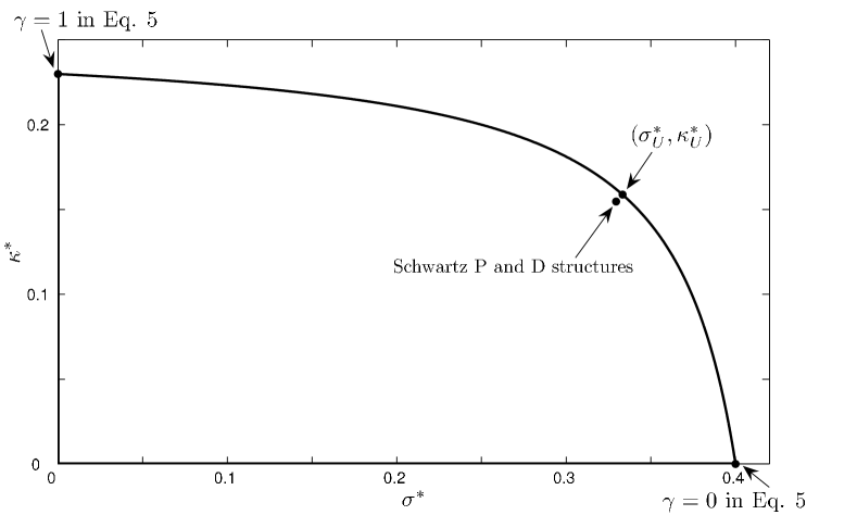
Figure 1: Effective properties of the $64,000$ voxel Schwartz P and D structures, the theoretical optimal point $(\sigma^{*}_{U},\kappa^{*}_{U})$ and the relevant cross–property bounds. The effective properties must lie within the region bounded by hyperbola shown and the $\sigma^{*}=0$ and $\kappa^{*}=0$ axes.

The conductive phase of the approximate Schwartz P and D structures is shown in Figs. 2 and 3 respectively. These figures also show the directional dependence of the effective Young’s modulus for the Schwartz P and D structures.

The effective Young’s modulus $E^{*}$ in a particular direction can be measured by loading the material uniaxially along that direction. $E^{*}$ is then the value of the applied stress divided by the resulting strain as measured along the loaded direction. Once the effective elasticity tensor for the composite has been calculated its Young’s modulus can be readily determined for any direction. We define $E_{min}^{*}$ and $E_{max}^{*}$ as the value of the effective Young’s modulus along the directions for which it is smallest and largest respectively.

Table 1 tabulates the calculated properties of $64,000$ voxel approximations of the Schwartz P and D structures.

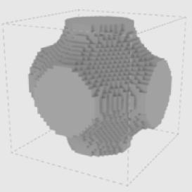
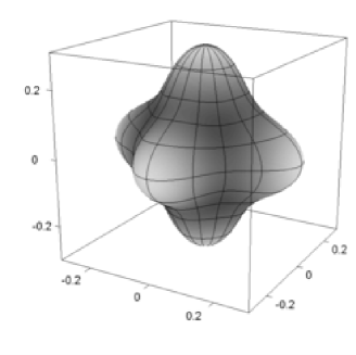
Figure 2: The conductive phase of the $64,000$ voxel approximation to a Schwartz P structure (left), and the directional dependence of its effective Young’s modulus (right).

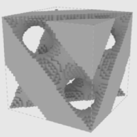
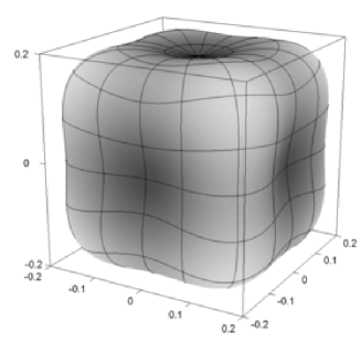
Figure 3: The conductive phase of the $64,000$ voxel approximation to a Schwartz D structure (left), and its calculated effective Young’s modulus for all directions (right).

Table 1: Effective properties of the approximate Schwartz P and D structures pictured in Figs. 2 and 3.

Structure	$\sigma^{*}$	$\kappa^{*}$	$\mathcal{A}$	$E^{*}_{min}$	$E^{*}_{max}$
Schwartz P	0.3288	0.1542	0.1925	0.1918	0.3040
Schwartz D	0.3302	0.1551	0.1635	0.1800	0.2795

Notes: $\mathcal{A}$ is the anisotropy of the structure, as defined in Section 3.

2.4 Motivation for the isotropy constraint

Figs. 2 and 3 clearly show the anisotropic stiffness properties of the Schwartz P and D structures. This is also demonstrated by the large difference between $E_{min}^{*}$ and $E_{max}^{*}$ for the two structures, as tabulated in Table 1. In many engineering applications the presence of weak directions would not be favourable. We note that the Schwartz P and D structures have cubic symmetry and therefore are isotropic with respect to conductivity. Structures without cubic symmetry have directions with low conductivity, this would also not be desirable in some cases. An isotropy constraint is an obvious suggestion to ensure that the Young’s modulus and conductivity are the same in all directions. In such a case the picture corresponding to the right hand picture in Figs. 2 and 3 would be a sphere with radius $E^{*}$.

More precisely, the two following intuitive result holds.

2.4.1 Result

Given isotropic and anisotropic microstructures with the same average value of any directional property $X^{*}$, the isotropic microstructure has the largest $X_{min}^{*}$.

2.4.2 Proof

The property $X^{*}$ is averaged over all directions for the anisotropic microstructure to give $\bar{X^{*}}$:

$$\bar{X^{*}}=\frac{1}{4\pi}\int_{\theta=0}^{2\pi}\int_{\phi=0}^{\pi}X^{*}(\theta,\phi)\sin(\phi)\mathrm{d}\phi\mathrm{d}\theta,$$ (6)

where $\theta$ and $\phi$ are the standard azimuthal and polar angles respectively. Since $\bar{X^{*}}$ is the average of $X^{*}$ for all directions and the microstructure is not isotropic, there must exist a direction for which $X^{*}<\bar{X^{*}}$. Thus $X_{min}^{*,aniso}<\bar{X^{*}}$.

Since the isotropic microstructure has this same $\bar{X^{*}}$ and is isotropic, $X^{*,iso}=\bar{X^{*}}$ for all directions. Obviously $X_{min}^{*,iso}=\bar{X^{*}}$.

We obtain $X_{min}^{*,aniso}<\bar{X^{*}}=X_{min}^{*,iso}$, proving the result.

3 Topology optimization algorithm

3.1 Calculation of effective properties

We use the standard elastic homogenization approach, for example see Garboczi and Day (1995) and the references therein, and choose to write it simply as

$$\sigma^{*}_{ij}=A_{ijkl}^{*}\epsilon^{*}_{kl},$$ (7)

where $\sigma_{ij}^{*}$ represents the effective stress tensor (not to be confused with $\sigma^{*}$ which represents the effective conductivity) and $\epsilon^{*}_{kl}$ represents the global strain tensor. The usual summation convention is used. The effective elasticity tensor $A_{ijkl}^{*}$ can be calculated by applying six independent strain fields corresponding to the six independent components of the symmetric strain tensor. These strains are applied to the unit cell with periodic boundary conditions. The resulting stresses are found using the finite element method and are averaged over the voxels to give the components of the elasticity tensor.

Similarly for the conductivity case,

$$J^{*}_{i}=K_{ij}^{*}E^{*}_{j},$$ (8)

where $J^{*}_{i}$ is the effective current vector and $E^{*}_{i}$ is the global applied electric field. The effective conductivity tensor $K_{ij}^{*}$ is calculated by applying three independent electric fields to the unit cell with periodic boundary conditions. The electric currents are computed by solving Laplace’s equation with the finite element method and are averaged over the voxels in the finite element mesh to give the components of the conductivity tensor.

We use the following definitions of the effective bulk modulus and shear modulus:

$$\kappa^{*} = \frac{1}{9}A^{*}_{iijj},$$ (9)

$$\mu^{*} = \frac{1}{20}\left(A^{*}_{ijij}+A^{*}_{ijji}\right)-\frac{1}{30}A^{*}_{iijj},$$ (10)

which are invariants of the effective elasticity tensor and are certainly correct for the isotropic case in Eq. 2.

Similarly, the following is our definition of the effective conductivity

$$\sigma^{*}=\frac{1}{3}K_{ii}^{*}.$$ (11)

3.2 Measuring anisotropy

We measure elastic anisotropy as the “distance” between the calculated $A_{ijkl}^{*}$ and the “nearest” isotropic elasticity tensor $A_{ijkl}^{*,iso}$:

$$\mathcal{A}_{mech}=\sqrt{\frac{\left(A_{ijkl}^{*}-A_{ijkl}^{*,iso}\right)\left(A_{ijkl}^{*}-A_{ijkl}^{*,iso}\right)}{A_{\bar{i}\bar{j}\bar{k}\bar{l}}^{*,iso}A_{\bar{i}\bar{j}\bar{k}\bar{l}}^{*,iso}}},$$ (12)

with $A_{ijkl}^{*,iso}$ given in Eq. 2 using effective properties from Eqs. 9 and 10. The denominator can be simplified to $9\kappa^{*2}+20\mu^{*2}$.

Similarly, we measure conductive anisotropy as

$$\mathcal{A}_{cond}=\sqrt{\frac{\left(K_{ij}^{*}-K_{ij}^{*,iso}\right)\left(K_{ij}^{*}-K_{ij}^{*,iso}\right)}{K_{\bar{i}\bar{j}}^{*,iso}K_{\bar{i}\bar{j}}^{*,iso}}},$$ (13)

where $K_{ij}^{*,iso}$ is as in Eq. 3 with $\sigma^{*}$ defined in Eq. 11. The denominator simplifies to $3\sigma^{*2}$.

As an overall anisotropy measure these two individual anisotropies are summed to give

$$\mathcal{A}=\mathcal{A}_{mech}+\mathcal{A}_{cond}.$$ (14)

3.3 Isotropy constraints

The numerators of $\mathcal{A}_{mech}^{2}$ and $\mathcal{A}_{cond}^{2}$ are sums of squares. To impose $\mathcal{A}=0$ a constraint is introduced for each term in the sum. For example, in the conductivity case the six constraints are $C_{p},p\in\{1,\dots,6\}$, where

$$\sqrt{3}\sigma^{*}C_{1} = K_{11}^{*}-\sigma^{*},$$

$$\sqrt{3}\sigma^{*}C_{2} = K_{22}^{*}-\sigma^{*},$$

$$\sqrt{3}\sigma^{*}C_{3} = K_{33}^{*}-\sigma^{*},$$

$$\sqrt{3}\sigma^{*}C_{4} = \sqrt{2}K_{12}^{*},$$

$$\sqrt{3}\sigma^{*}C_{5} = \sqrt{2}K_{13}^{*},$$

$$\sqrt{3}\sigma^{*}C_{6} = \sqrt{2}K_{23}^{*}.$$ (15)

Only five of these are independent but we work with all six to explicitly retain symmetry in the numerical calculations. The factors of $\sqrt{2}$ are included in $C_{4}$, $C_{5}$ and $C_{6}$ on the right hand side and the factors of $\sqrt{3}\sigma^{*}$ are included on the left hand side to give $\mathcal{A}_{cond}^{2}=\sum_{p=1}^{6}C_{p}^{2}$.

Similarly $21$ constraints $C_{p},p\in\{7,\dots,27\}$ can be written down for the elasticity case, $19$ of which are independent. They are also normalized so that summing and squaring them gives $\mathcal{A}_{mech}^{2}$.

3.4 Level–set method for topology optimization

Topological optimization is implemented using the level–set approach formalized by Allaire et al. (2004) and Wang et al. (2003) and based on earlier work by Osher and Santosa (2001) and Sethian and Wiegmann (2000). The reader is referred to Allaire et al. (2004) for standard details of the level–set approach; only significant deviations from the standard method are mentioned here. Note that the topological derivative, as used for example by Allaire et al. (2005), is not used in the work presented here. We have found that, as noted by Allaire et al. (2004), topological changes are readily achieved using the level–set method in three dimensions without the topological derivative, rendering it unnecessary.

In our implementation the level–set function is initialized using an approximation to the signed distance function, found by finding the nearest voxel of opposite phase with respect to the standard metric on $\mathbb{R}^{3}$. This initialization procedure is also used to reinitialize the level–set function at each iteration of the algorithm.

The Hamilton–Jacobi evolution equation is solved via a standard upwind scheme and the time–step for the numerical evolution must be less than that given by the Courant–Friedrichs–Lewy (CFL) condition to ensure numerical stability (Sethian, 1999). We choose to use a time–step 1% of the CFL value and do many level–set evolutions per iteration of the optimization algorithm, typically between 25 and 100. The number of level–set evolutions per iteration is gradually reduced as the optimization converges to a local minimum.

The shape derivatives of the effective elasticity and conductivity tensor components $A_{ijkl}^{*}$ and $K_{ij}^{*}$ are readily computed from well–known shape derivatives (see Allaire et al., 2004, and the references therein) by utilizing the superposition principle for strains and stresses in linear elasticity and electric fields and currents in conductivity. From these it is straightforward to calculate the shape derivatives of the constraints and of the effective properties $\kappa^{*}$ and $\sigma^{*}$ to give the shape derivative of the objective function. These are of the form

$$\frac{\mathrm{d}J}{\mathrm{d}\Omega}(\theta) = -\int_{\partial\Omega}\theta_{i}n_{i}v,$$

$$\frac{\mathrm{d}C_{p}}{\mathrm{d}\Omega}(\theta) = -\int_{\partial\Omega}\theta_{i}n_{i}v_{p}\quad p\in\{1,\dots,27\}.$$ (16)

Here $\Omega$ is the region occupied by the stiff phase. It is being deformed by the map $x_{i}\rightarrow x_{i}+\theta_{i}$, so the left hand side of each equation above is the standard shape derivative. The boundary of $\Omega$ is $\partial\Omega$, with outward normal $n_{i}$. The quantities $v$ and $v_{p}$ are called the shape sensitivities of $J$ and $C_{p}$.

3.5 Imposing the isotropy constraints

In the situation with no constraints, $\theta_{i}$ is often chosen to be $\theta_{i}=vn_{i}$, and the normal velocity $\mathcal{V}$ of the phase interface is chosen as $\mathcal{V}=\theta_{i}n_{i}=v$. This implements a steepest descent type algorithm under evolution with the Hamilton–Jacobi equation. A modification of this for the constrained case is outlined below. A more detailed presentation is given in Wilkins et al. (2007).

At any generic iteration of the algorithm, the constraints will be nonzero. To reduce both the objective function and the constraints we can require:

$$\int_{\partial\Omega}\theta_{i}n_{i}v = \mbox{maximum possible},$$ (17)

$$\int_{\partial\Omega}\theta_{i}n_{i}v_{p} = rC_{p}\ \quad p\in\{1,\dots,27\},$$ (18)

where $r$ dictates the rate of exponential decay of the constraints.

The shape sensitivities are functions defined on $\partial\Omega$ and may be thought of as elements of a Hilbert space. In the following, the notation $||\cdot||$ and $\langle\cdot,\cdot\rangle$ is short hand for the norm and inner product on $\partial\Omega$: $||v_{p}||^{2}=\int_{\partial\Omega}v_{p}^{2}$, $\langle v_{p},v_{q}\rangle=\int_{\partial\Omega}v_{p}v_{q}$. In the finite element implementation $\int_{\partial\Omega}v_{p}v_{q}$ is approximated by a sum over all the boundary voxels of the product $v_{p}v_{q}$. A voxel is determined as a boundary voxel if any of its 26 neighbours (including those across periodic boundaries) are of the opposite phase.

Linearly dependent $\{v_{p}\}$ are removed from the set. We use the Gram-Schmidt procedure to build a mutually orthogonal set $\{\bar{v}_{p}:p\in\{1,\dots,24\}\}$ from $\{v_{p}\}$ which spans the constraint shape sensitivities. From this we can form the projection operator $P$ which projects vectors in $\partial\Omega$ onto the space which will leave the constraints invariant.

To implement Eq. 18 we take

$$\mathcal{V}=\theta_{i}n_{i}=\sqrt{1-\sum_{p=1}^{24}\alpha_{p}^{2}}\frac{Pv}{||Pv||}+\sum_{p=1}^{24}\alpha_{p}\frac{\bar{v}_{p}}{||\bar{v}_{p}||}\ ,$$ (19)

where the $\alpha_{p}$ are real numbers which are chosen to solve the lower-diagonal system

$$\left(\begin{array}[]{c}rC_{1}\\ rC_{2}\\ rC_{3}\\ \vdots\\ rC_{24}\end{array}\right)=\left(\begin{array}[]{ccccc}||\bar{v}_{1}||&0&0&\ldots&0\\ \frac{\langle\bar{v}_{1},v_{2}\rangle}{||\bar{v}_{1}||}&||\bar{v}_{2}||&0&\ldots&0\\ \frac{\langle\bar{v}_{1},v_{3}\rangle}{||\bar{v}_{1}||}&\frac{\langle\bar{v}_{2},v_{3}\rangle}{||\bar{v}_{2}||}&||\bar{v}_{3}||&\ldots&0\\ \vdots&\vdots&\vdots&\ddots&0\\ \frac{\langle\bar{v}_{1},v_{24}\rangle}{||\bar{v}_{1}||}&\frac{\langle\bar{v}_{2},v_{24}\rangle}{||\bar{v}_{2}||}&\frac{\langle\bar{v}_{3},v_{24}\rangle}{||\bar{v}_{3}||}&\ldots&||\bar{v}_{24}||\end{array}\right)\left(\begin{array}[]{c}\alpha_{1}\\ \alpha_{2}\\ \alpha_{3}\\ \vdots\\ \alpha_{24}\end{array}\right).$$ (20)

In essence, this has decomposed $\theta_{i}n_{i}$ into the sum of two parts. The first part is orthogonal to the shape sensitivities. The second part is a linear combination of the shape sensitivities. The former has been chosen to decrease the objective function as in Eq. (17), while the latter has been chosen to decrease the constraints as in Eq. (18).

The parameter $r$ is chosen to ensure $1-\sum_{p}\alpha_{p}^{2}\geq 0$ and $\sum_{p}\alpha_{p}^{2}\geq\alpha_{min}^{2}$. Changing $\alpha_{min}^{2}$ effects how strongly the algorithm projects onto the constraints. Typically we choose $\alpha_{min}^{2}=0.1$.

3.6 Imposing the volume constraint

The volume constraint is imposed via the Karush–Khun–Tucker technique (Karush, 1939; Kuhn and Tucker, 1951). In our setting this technique involves calculating the expected volume change under evolution and if necessary correcting the shape derivative to ensure the volume change will not make the phase volume fractions deviate further from their required values. This type of technique has been used with the level–set method for topology optimization previously (Wang and Wang, 2006).

3.7 Velocity extension via smoothing

The above method for the isotropy constraints calculates the normal velocity $\mathcal{V}$ at all boundary voxels. The normal velocity is set to zero for all non–boundary voxels.

One issue with the level–set method of topology optimization is that the velocity must be extended away from the boundaries to give evolution of the structure. Frequently this is addressed by using an ersatz material approach, whereby material properties of the weak phase are set to some small nonzero value instead of to zero, see for example Allaire et al. (2004). We choose to apply a smoothing to the velocities via the convolution

$$\mathcal{V}_{i,j,k}\leftarrow\frac{1}{8}(2\mathcal{V}_{i,j,k}+\mathcal{V}_{i-1,j,k}+\mathcal{V}_{i+1,j,k}+\mathcal{V}_{i,j-1,k}+\mathcal{V}_{i,j+1,k}+\mathcal{V}_{i,j,k-1}+\mathcal{V}_{i,j,k+1}),$$ (21)

where the subscripts refer to indices of the voxels. This convolution is applied repeatedly until Hamilton–Jacobi evolution will result in a geometric change of the structure. We note that this smoothing operation allows us to use only two phases during the optimization: no intermediate densities are required.

4 Results

Any initial unit cell is suitable to start the optimization process provided the initial periodic material has nonzero stiffness and nonzero conductivity in all directions. All of the optimized structures presented are optimized from the initial unit cell shown in Fig. 4(a).

The chosen initial unit cell has two nice properties. First, the two phases have the same topology and geometry, meaning that there is no initial bias towards a particular property. Although the two phases of the initial unit cell look different in Fig. 4(a), a shift of either phase along each coordinate direction by half the unit cell edge length demonstrates that the two phases of the initial microstructure are geometrically identical. Second, the cell has simple cubic symmetry. Our computational approach retains this throughout the optimization and $\mathcal{A}_{cond}=0$ at each iteration. Isotropy with respect to elasticity is more difficult to achieve.

The choice of internal parameters in the algorithm effects the outcome of the optimization process. The differences are often insignificant and experience with the algorithm allows the user to find a small set of internal parameters to use on each optimization problem. Results presented reflect the optimized structure with the best objective function value from optimizations with various choices of internal parameters. It is not surprising that other inferior structures can be reached with different parameter choices: the level–set method converges to a local minimum and we do not know that a single global minimum exists.

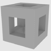
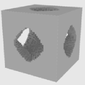
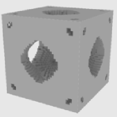
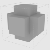
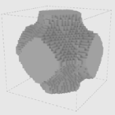
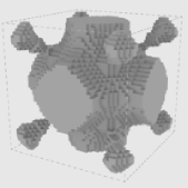
(a)                        (b)                        (c)                        (d)

Figure 4: An example optimization history with $(\bar{\omega}_{\kappa},\bar{\omega}_{\sigma})=(1,\frac{1}{2})$. The four columns are (a) the initial unit cell, (b) iteration 20, (c) iteration 55 and (d) the optimized unit cell. In each case the top and bottom picture show the stiff phase and conductive phase respectively.

4.1 Equal phase volume fractions

First we consider the design of unit cells with an equal volume fraction for each phase, i.e., $V_{1}=\frac{1}{2}=V_{2}$. Fig. 4 shows an initial structure, two intermediate structures and the optimized structure for $(\bar{\omega}_{\kappa},\bar{\omega}_{\sigma})=(1,\frac{1}{2})$. Fig. 4 highlights that no intermediate densities are used at any time in the optimization.

The material properties for the four microstructures shown in Fig. 4 are given in Table 2. Note that the volume constraint and the isotropy constraint are not satisfied during the optimization process. The errors on these constraints are small for the optimized structure (and for other optimized structures presented). We have seen that small geometric changes can produce large percentage changes in $\mathcal{A}$ when it is small, with corresponding very small changes in $V_{1}$, $V_{2}$ and the objective function. Thus we consider a value of $\mathcal{A}<0.005$ to be small enough for the isotropy constraint to be satisfied. Also, a value of $|V_{1}^{required}-V_{1}^{actual}|<0.0005$ is considered good enough given that the unit cells are represented with only $64,000$ voxels without intermediate densities.

Particularly of interest in Table 2 is how the minimum and maximum Young’s moduli $E_{min}^{*}$ and $E_{max}^{*}$ change throughout the optimization. As the optimization progresses and the anisotropy $\mathcal{A}$ decreases, the difference between the maximum and minimum Young’s moduli also decreases. For the optimized structure we see that the maximum and minimum Young’s moduli are less than 1% apart, highlighting the effectiveness of the isotropy constraint. This is the case for all optimized structures presented and therefore $E^{*}=\frac{9\kappa^{*}\mu^{*}}{3\kappa^{*}+\mu^{*}}$ is tabulated in the remainder of the paper.

Table 2: Effective properties of the four unit cells from the optimization history shown in Fig. 4.

Case	$J$	$\sigma^{*}$	$\kappa^{*}$	$V_{1}$	$\mathcal{A}$	$E^{*}_{min}$	$E^{*}_{max}$
(a)	-0.3016	0.3170	0.1432	0.5000	0.2826	0.1444	0.2951
(b)	-0.3063	0.3261	0.1432	0.5109	0.1806	0.1901	0.2885
(c)	-0.3170	0.2987	0.1676	0.5194	0.0909	0.2322	0.2902
(d)	-0.3187	0.3226	0.1574	0.5003	0.0029	0.2373	0.2389

Optimized unit cells for different $(\bar{\omega}_{\kappa},\bar{\omega}_{\sigma})$ pairs are shown in Fig. 5. The effective properties for these optimized microstructures are given in Table 3. Fig. 6 shows the effective bulk modulus and conductivity for the optimized structures along with the cross–property bounds for the correct volume fractions and phase properties. The optimized structures are very close to the cross–property bounds and structures at several points along the bounds were readily obtained by changing the coefficients $\bar{\omega}_{\kappa}$ and $\bar{\omega}_{\sigma}$ in the objective function. We note that Fig. 5(a) resembles the isotropic, maximum bulk modulus structure presented by Sigmund (2000).

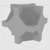
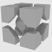
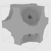
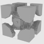
(a)                                                          (b)

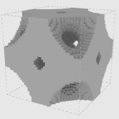
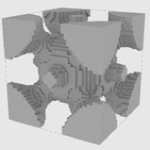
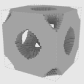
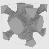
(c)                                                          (d)

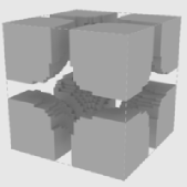
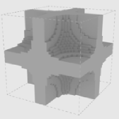
(e)

Figure 5: Optimized unit cells with $V_{1}=\frac{1}{2}$ and different weighting schemes in the objective function: (a) $(\bar{\omega}_{\kappa},\bar{\omega}_{\sigma})=(1,0)$, (b) $(\bar{\omega}_{\kappa},\bar{\omega}_{\sigma})=(1,\frac{1}{10})$, (c) $(\bar{\omega}_{\kappa},\bar{\omega}_{\sigma})=(1,\frac{1}{6})$, (d) $(\bar{\omega}_{\kappa},\bar{\omega}_{\sigma})=(1,\frac{1}{2})$, (e) $(\bar{\omega}_{\kappa},\bar{\omega}_{\sigma})=(0,1)$. In each case the left and right picture show the stiff phase and conductive phase respectively.

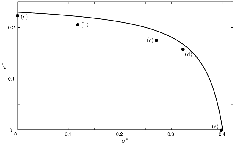
Figure 6: Effective properties for the optimized structures with $V_{1}=\frac{1}{2}$ given in Fig. 5. The curve indicates the cross-property bounds for the problem.

Table 3: Effective properties of the five optimized structures with $V_{1}=\frac{1}{2}$ shown in Fig. 5.

Case	$(\bar{\omega}_{\kappa},\bar{\omega}_{\sigma})$	$J$	$\sigma^{*}$	$\kappa^{*}$	$V_{1}$	$\mathcal{A}$	$E^{*}$	$g$
(a)	$(1,0)$	-0.2231	0.0000	0.2231	0.5000	0.0003	0.3039	0
(b)	$(1,\frac{1}{10})$	-0.2170	0.1174	0.2053	0.4999	0.0014	0.2857	7
(c)	$(1,\frac{1}{6})$	-0.2201	0.2709	0.1749	0.4999	0.0013	0.2547	10
(d)	$(1,\frac{1}{2})$	-0.3187	0.3226	0.1574	0.5003	0.0029	0.2379	10
(e)	$(0,1)$	-0.3971	0.3971	0.0000	0.4996	0.0000	0.0000	0

Note: $g$ is the genus per unit cell, see Section 5.

4.2 30% stiff volume fraction

To further explore the capabilities of the level–set method for microstructure design and the near–optimal structures for the stiffness–conductivity problem, a study similar to the above was performed with a required stiff phase volume fraction of $V_{1}=\frac{3}{10}$. Optimized structures for $V_{1}=\frac{3}{10}$ and different coefficients in the objective function are presented in Fig. 7. The effective properties for these structures are given in Table 4 and are summarized alongside the correct cross–property bounds in Fig. 8.

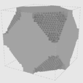
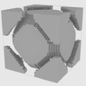
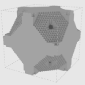
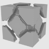
(a)                                                          (b)

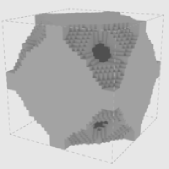
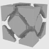
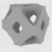
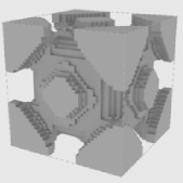
(c)                                                          (d)

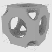
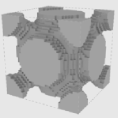
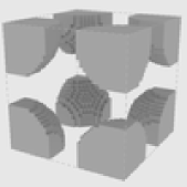
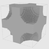
(e)                                                          (f)

Figure 7: Optimized unit cells with $V_{1}=\frac{3}{10}$ and different weighting schemes in the objective function: (a) $(\bar{\omega}_{\kappa},\bar{\omega}_{\sigma})=(1,0)$, (b) $(\bar{\omega}_{\kappa},\bar{\omega}_{\sigma})=(1,\frac{1}{50})$, (c) $(\bar{\omega}_{\kappa},\bar{\omega}_{\sigma})=(1,\frac{1}{20})$, (d) $(\bar{\omega}_{\kappa},\bar{\omega}_{\sigma})=(1,\frac{1}{10})$, (e) $(\bar{\omega}_{\kappa},\bar{\omega}_{\sigma})=(1,\frac{1}{2})$, (f) $(\bar{\omega}_{\kappa},\bar{\omega}_{\sigma})=(0,1)$. In each case the left and right picture show the stiff phase and conductive phase respectively.

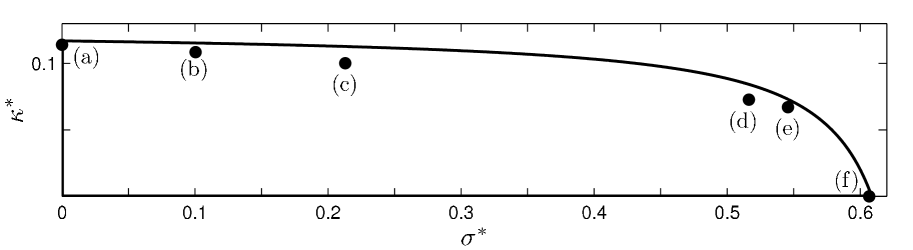
Figure 8: Effective properties for the optimized structures with $V_{1}=\frac{3}{10}$ given in Fig. 7. The curve indicates the cross-property bounds for the problem.

Table 4: Effective properties of the optimized structures with $V_{1}=\frac{3}{10}$ shown in Fig. 7.

Case	$(\bar{\omega}_{\kappa},\bar{\omega}_{\sigma})$	$J$	$\sigma^{*}$	$\kappa^{*}$	$V_{1}$	$\mathcal{A}$	$E^{*}$	$g$
(a)	$(1,0)$	-0.1140	0.0000	0.1140	0.3000	0.0022	0.1459	0
(b)	$(1,\frac{1}{50})$	-0.1105	0.1004	0.1085	0.3000	0.0004	0.1383	7
(c)	$(1,\frac{1}{20})$	-0.1108	0.2129	0.1001	0.3004	0.0009	0.1309	7
(d)	$(1,\frac{1}{10})$	-0.1243	0.5163	0.0727	0.3000	0.0039	0.1006	10
(e)	$(1,\frac{1}{2})$	-0.3399	0.5457	0.0671	0.2996	0.0011	0.0987	10
(f)	$(0,1)$	-0.6069	0.6069	0.0000	0.2998	0.0000	0.0000	0

4.3 70% stiff volume fraction

This section presents optimized structures with a required stiff phase volume fraction of $V_{1}=\frac{7}{10}$. Optimized structures are displayed in Fig. 9. Effective properties for the optimized structures are presented in Table 5 and summarized alongside the cross–property bounds in Fig. 10.

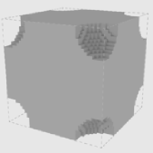
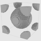
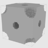
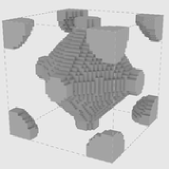
(a)                                                          (b)

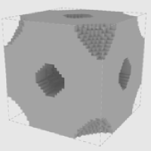
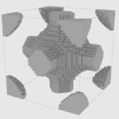
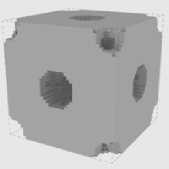
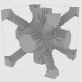
(c)                                                          (d)

Figure 9: Optimized unit cells with $V_{1}=\frac{7}{10}$ and different weighting schemes in the objective function: (a) $(\bar{\omega}_{\kappa},\bar{\omega}_{\sigma})=(1,0)$, (b) $(\bar{\omega}_{\kappa},\bar{\omega}_{\sigma})=(1,\frac{1}{3})$, (c) $(\bar{\omega}_{\kappa},\bar{\omega}_{\sigma})=(1,\frac{1}{2})$, (d) $(\bar{\omega}_{\kappa},\bar{\omega}_{\sigma})=(1,1)$. In each case the left and right picture show the stiff phase and conductive phase respectively.

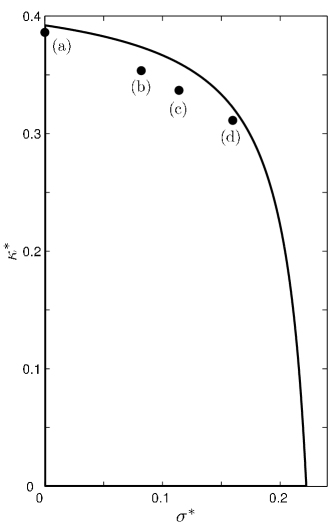
Figure 10: Effective properties for optimized structures with $V_{1}=\frac{7}{10}$ given in Fig. 9. The curve indicates the cross-property bounds for the problem.

Table 5: Effective properties of the optimized structures with $V_{1}=\frac{7}{10}$ shown in Fig. 9.

Case	$(\bar{\omega}_{\kappa},\bar{\omega}_{\sigma})$	$J$	$\sigma^{*}$	$\kappa^{*}$	$V_{1}$	$\mathcal{A}$	$E^{*}$	$g$
(a)	$(1,0)$	-0.3861	0.0000	0.3861	0.6998	0.0001	0.5234	0
(b)	$(1,\frac{1}{3})$	-0.3808	0.0819	0.3536	0.6999	0.0006	0.4940	3
(c)	$(1,\frac{1}{2})$	-0.3938	0.1140	0.3368	0.7003	0.0004	0.4762	3
(d)	$(1,1)$	-0.4710	0.1597	0.3113	0.7001	0.0012	0.4547	10

5 Discussion

The optimized structures with $V_{1}=\frac{1}{3}$ display the same set of topologies as the optimized structures with $V_{1}=\frac{1}{2}$. The optimized structures for both cases have effective properties very close to the cross–property bounds.

As in Fig. 4, it is frequently the conductive phase which extends out to make new topologies in the optimization process. Accordingly, it was more difficult to obtain optimized structures close to the cross–property bounds for the $V_{1}=\frac{7}{10}$ case. We see familiar topologies from the other volume fraction cases for structures (a) and (d) in Fig. 9. However, along the low conductivity section of the curve the optimized structures ((b) and (c) in Fig. 9) have a conductive phase which is in two disconnected parts. One part of the conductive phase provides effective conductivity whereas the other is present to satisfy the isotropy constraint.

For all three volume fraction cases we have been unable to obtain structures in the high–conductivity part of the cross–property bounds curve which have nonzero stiffness. For example, see the gap between structures (d) and (e) in Fig. 6. We believe this problem stems from the isotropy constraint: for a small effective stiffness the algorithm simply disconnects the stiff phase to make it trivially isotropic. Aiming for this section of the curve $\bar{\omega}_{\sigma}>\bar{\omega}_{\kappa}$ in the objective function, thus zero stiffness does not affect the objective function significantly. Structures in this region may be found by using an objective function which includes a penalty for disconnecting each of the phases, e.g., $J=\frac{\omega_{\kappa}}{\kappa^{*}}+\frac{\omega_{\sigma}}{\sigma^{*}}$. Alternatively, significant experimentation with $\alpha_{min}^{2}$ may give structures with the desired properties.

For the $V_{1}=\frac{7}{10}$ case we were also unable to obtain a structure close to $(\sigma_{HS},0)$. The geometry expected for this structure given those obtained for the other volume fraction cases appears impossible at $V_{1}=\frac{7}{10}$. Swapping the phases of structure (a) from Fig. 7, which has $V_{1}=\frac{3}{10}$ and properties close to $(0,\kappa_{HS})$, would give a structure very close to $(\sigma_{HS},0)$ on the $V_{1}=\frac{7}{10}$ cross–property bounds. However, it is the isotropy requirement for the elastic phase which drives the algorithm to the body–centered arrangement of Fig. 7(a). Given that the algorithm moves towards disconnecting the stiff phase, the optimization is not driven towards the correct structure. Instead it tends towards the simple cubic structure seen at other volume fractions, and when it is unable to disconnect the stiff phase cannot then move towards the body–centered geometry.

In Fig. 11 we hypothesize the existence of optimal microstructures with the topologies of the optimized microstructures we have presented. The microstructures are grouped based on their topology using the genus $g$ which represents the number of handles of an object (Hyde, 1989).

Figure 11: The effective properties of optimal stiff and conducting microstructures for all volume fractions (above) and a parameterization of this surface using the stiff phase volume fraction $V_{1}$ and the parameter $\gamma$ from Eq. 5 (below). In each case the black dots correspond to particular microstructures inferred from the optimized structures we have presented. The lower “phase–diagram” is divided into areas for which we hypothesize the existence of optimal microstructures with a particular topology. The three vertical dotted lines represent the three stiff phase volume fractions considered in this paper. Solid lines represent boundaries between regions, but should be considered as approximate. Dashed lines represent the extent of what we can infer from the optimized structures presented. Corresponding regions can be seen on the surface in the upper diagram.

6 Concluding remarks

This paper presents a method for material design using the level–set method of topology optimization. The method is utilized to design isotropic periodic composite materials in three dimensions which are maximally stiff and conducting from two ill–ordered, infinite contrast phases. The optimized microstructures presented here have properties very close to the relevant conductivity bulk modulus cross–property bounds, proving the capabilities of the level–set method for microstructure design.

Until now, the only known optimal single–scale microstructures for this problem are cubic symmetric and therefore have weak directions. An important component of our method is the ability to improve upon this by imposing an isotropy constraint. The isotropy of the optimized microstructures makes them attractive for engineering applications: provided the shear modulus of the microstructures is high, the composites will have a high Young’s modulus in all directions. The isotropy requirement means that almost all of our optimized microstructures have not been presented previously. Our method can readily be applied to other constraints.

For various volume fractions we hypothesize the existence of optimal single–scale microstructures with the topologies of those presented. We have not been able to find near–optimal structures for the high–conductivity nonzero stiffness section of the cross–property diagram. This is a result of the the isotropy constraint; instead of constraining the microstructures to be isotropic while being only weakly stiff the algorithm disconnects the stiff phase to make it trivially isotropic.

The freedom to choose the initial unit cell has not been discussed. Different initial cells can give different prescribed symmetries and preliminary investigations demonstrate that different initial cells will almost certainly result in different optimized microstructures close to the cross–property bounds. Thus there are possibly other microstructures with similar properties to those presented; this would provide the designer with freedom to choose the microstructure to suit their purposes. However, given the closeness of our optimized structures to the cross–property bounds, other microstructures found could not outperform them by much more than a few percent.

References

- Allaire et al. (2005) Allaire, G., de Gournay, F., Jouve, F., Toader, A.-M., 2005. Structural optimization using topological and shape sensitivity via a level set method. Control and Cybernetics 34 (1), 59–80.
- Allaire et al. (2004) Allaire, G., Jouve, F., Toader, A.-M., 2004. Structural optimization using sensitivity analysis and a level-set method. J. Comput. Phys. 194, 363–393.
- Bendsøe (1989) Bendsøe, M. P., 1989. Optimal shape design as a material distribution problem. Struct. Opt. 1, 193–202.
- Bendsøe and Kikuchi (1988) Bendsøe, M. P., Kikuchi, N., 1988. Generating optimal topologies in structural design using a homogenization method. Comput. Methods Appl. Mech. Engng. 71, 197–224.
- de Kruijf et al. (2007) de Kruijf, N., Zhou, S., Li, Q., Mai, Y.-W., 2007. Topological design of structures and composite materials with multiobjectives. International Journal of Solids and Structures 44, 7092–7109.
- Garboczi and Day (1995) Garboczi, E. J., Day, A. R., 1995. An algorithm for computing the effective linear elastic properties of heterogeneous materials: three-dimensional results for composites with equal phase poisson ratios. J. Mech. Phys. Solids 43, 1349–1362.
- Gibiansky and Torquato (1996) Gibiansky, L., Torquato, S., 1996. Connection between the conductivity and bulk modulus of isotropic composite materials. Proc. R. Soc. Lond. A 452, 253–283.
- Guest and Prévost (2006) Guest, J., Prévost, J. H., 2006. Optimizing multifunctional materials: Design of microstructures for maximized stiffness and fluid permeability. Int. J. Solids and Structures 43, 7028–7047.
- Hashin and Shtrikman (1962) Hashin, Z., Shtrikman, S., 1962. A variational approach to the theory of the effective magnetic permeability of multiphase materials. J. Appl. Phys. 35, 3125–3131.
- Hashin and Shtrikman (1963) Hashin, Z., Shtrikman, S., 1963. A variational approach to the theory of the elastic behaviour of multiphase materials. J. Mech. Phys. Solids 11, 127–140.
- Hyde (1989) Hyde, S., 1989. The topology and geometry of infinite periodic surfaces. Z. Kristallogr. 187, 165–185.
- Karush (1939) Karush, W., 1939. Minima of functions of several variables with inequalities as side constraints. Master’s thesis, Dept. Math, Univ. of Chicago, Illinois.
- Kuhn and Tucker (1951) Kuhn, H., Tucker, A., 1951. Nonlinear programming. In: Proceedings of 2nd Berkeley Symposium. University of California Press, Berkeley, pp. 481–492.
- Osher and Santosa (2001) Osher, S. J., Santosa, F., 2001. Level set methods for optimization problems involving geometry and constraints I. frequencies of a two–density inhomogeneous drum. J. Comput. Phys. 171, 272–288.
- Sethian (1999) Sethian, J. A., 1999. Level set methods and fast marching methods, Evolving interfaces in computational geometry, fluid mechanics, computer vision and materials science, 2nd Edition. Cambridge University Press.
- Sethian and Wiegmann (2000) Sethian, J. A., Wiegmann, A., 2000. Structural boundary design via level set and immersed interface methods. J. Comput. Phys. 163 (2), 489–528.
- Sigmund (2000) Sigmund, O., 2000. A new class of extremal composites. Journal of the Mechanics and Physics of Solids 48, 397–428.
- Torquato and Donev (2004) Torquato, S., Donev, A., 2004. Minimal surfaces and multifunctionality. Proc. R. Soc. Lond. A 460, 1849–1856.
- Torquato et al. (2002) Torquato, S., Hyun, S., Donev, A., 2002. Multifunctional composites: Optimizing microstructures for simultaneous transport of heat and electricity. Phys. Rev. Lett. 89, 266601–1–4.
- Torquato et al. (2003) Torquato, S., Hyun, S., Donev, A., 2003. Optimal design of manufacturable three-dimensional composites with multifunctional characteristics. J. Appl. Phys. 94, 5748–5755.
- Wang et al. (2003) Wang, M. Y., Wang, X., Guo, D., 2003. A level set method for structural topology optimization. Comput. Meth. Appl. Mech. Engrg. 192, 227–246.
- Wang and Wang (2006) Wang, S. Y., Wang, M. Y., 2006. A moving superimposed finite element method for structural topology optimization. Int. J. Numer. Methods Eng. 65, 1892–1922.
- Wilkins et al. (2007) Wilkins, A. H., Challis, V. J., Roberts, A. P., 2007. Isotropic, stiff, conducting structures via topology optimization. In: Proceedings of the 7th World Congress on Structural and Multidisciplinary Optimization.