Coulomb correlation in presence of spin-orbit coupling: application to plutonium

Abstract

Attempts to go beyond the local density approximation (LDA) of Density Functional Theory (DFT) have been increasingly based on the incorporation of more realistic Coulomb interactions. In their earliest implementations, methods like LDA+$U$, LDA + DMFT (Dynamical Mean Field Theory), and LDA+Gutzwiller used a simple model interaction $U$. In this article we generalize the solution of the full Coulomb matrix involving $F^{(0)}$ to $F^{(6)}$ parameters, which is usually presented in terms of an $\ell m_{\ell}$ basis, into a $jm_{j}$ basis of the total angular momentum, where we also include spin-orbit coupling; this type of theory is needed for a reliable description of $f$-state elements like plutonium, which we use as an example of our theory. Close attention will be paid to spin-flip terms, which are important in multiplet theory but that have been usually neglected in these kinds of studies. We find that, in a density-density approximation, the $jm_{j}$ basis results provide a very good approximation to the full Coulomb matrix result, in contrast to the much less accurate results for the more conventional $\ell m_{\ell}$ basis.

I Introduction

Strongly correlated electron systems are solids where the important outer-shell electrons have two conflicting and opposite tendencies. On one hand, they maintain a strong memory of the atomic or localized orbitals from which they arise, which have a large electron-electron electrostatic interaction between discrete states. On the other hand, the same electrons hybridize with neighboring orbitals causing them to delocalize by tunnelling from one atom to those nearby, forming chemical bonds and spreading out the discrete atomic states into narrow energy bands. In such systems, it is therefore necessary for a correct description and understanding of their electronic properties to maintain both of these aspects. The second tendency is very accurately calculated by density functional theory (DFT) band-structure calculations, while the first one involves a consideration of many-body effects, and, while more difficult to treat, is still a crucial aspect of the physics. Thus, it is important to increase our knowledge of the Coulomb interactions that strongly affect the atomic character of these systems, an effect which is often underestimated or poorly approximated in calculations that include details of the band-structure.

These types of effects are particularly important for the electronic structure of $f$-electron elements in general, and especially for the actinides. For these materials, density functional theory (DFT) calculations in the local density approximation (LDA) Hohenberg64 ; Kohn65 often give significant discrepancies. For example, $\delta$-Pu from this kind of approach is predicted to have an equilibrium volume 25% smaller than experiment, which is the largest known deviation from LDA. To overcome these difficulties, various attempts to go beyond LDA have been proposed, such as LDA+$U$, Anisimov91 ; Bouchet00 LDA+DMFT,  Georges96 ; Anisimov97 ; Savrasov00 and more recently LDA+Gutzwiller. JulienBouchet06 All three of these methods add a local Hubbard-like term to a band Hamiltonian, and require subtraction of an average LDA Coulomb interaction (the double counting correction). The differences between the various methods reside in the way the effects of this interaction term is handled.

In the LDA+$U$ approach, which employs a Hartree-Fock mean-field solution, the Hubbard term leads to an orbital-dependent shift in the potential. Such a crude mean-field approximation is questionable for cases involving strong correlations. In the LDA+Gutzwiller method, a variational wavefunction is built, for which the mean values of the interaction are calculated exactly. In the more sophisticated DMFT method, the effect of the interaction is described by a self-energy, which acts as an energy-dependent complex potential. In this approximation the self-energy is assumed to be local (i.e., momentum independent) and is determined self-consistently within an impurity-like approach of a correlated site embedded in a effective bath. In many DMFT calculations the Hubbard-like term, at least in the early implementation of these methods, has often been treated in a fairly simplistic way. For example, some applications use a single $U$ term, average over all interactions, while others also include an exchange-averaged parameter $J$. Over time the general tendency for all three methods has been to include more and more realistic interactions. For example, since its first use, the LDA+$U$ has usually been rotationally invariant. rotinvLDA+U However, a multiband version of Gutzwiller approach developped by Bünemann, Gebhard and Weber Bunemann98b was able to handle spin-flip terms and very recently, a multiband generalization of slave-boson formalism Kotliar86 has been proposed to be rotationally invariant. rotinvSB To make progress, it is clearly important to develop a more sophisticated treatment of the Coulomb interactions. In addition, for high-Z materials like the $f$-electron actinides, spin-orbit must also be accurately included. To do this is the goal of this article.

The paper is organized as follows. Section II is devoted to the presentation of Coulomb matrix elements in the $jm_{j}$ basis. In this section, we first formulate a general expression for the interactions. We then show how to make an approximate density-density correlation calculation for these interactions. The corresponding matrix elements will be tabulated in terms of Slater integrals. Section III presents the eigen-spectrum of the atomic Hamiltonian in various different approximations. In Section IV we use these eigenvalues to study the single particle spectral density. In particular, the quality of various approximations will be evaluated against a rigorous solution. Finally, we conclude in Section V by stressing the main results of our approach.

II Coulomb matrix elements in the $jm_{j}$ basis

II.1 Electronic structure of an isolated atom

The Hamiltonian $H$ of an isolated many-electron atom or ion is

$$H=\sum_{i=1}^{N}\biggl{(}\frac{-\hbar^{2}}{2m}\nabla_{i}^{2}-\frac{Ze^{2}}{r_{i}}+\xi(r_{i})\overrightarrow{L_{i}}\cdot\overrightarrow{S_{i}}\biggr{)}+\sum_{i>j}\frac{e^{2}}{|r_{i}-r_{j}|}\;.$$ (1)

Beside the interaction of the electrons with the positive charge (Z) of the nucleus, this Hamiltonian contains two important features: the spin-orbit coupling and the electrostatic (Coulomb) interaction between electrons. By neglecting spin-orbit, in the central field approximation, CondonShortley the eigenstates of the system are Slater determinants built from individual states $|n\ell m_{\ell}sm_{s}\rangle$ having the following wave function:

$$\phi_{n\ell m_{\ell}sm_{s}}(r,\theta,\varphi)=\frac{R_{n\ell}(r)}{r}Y_{\ell m_{\ell}}(\theta,\varphi)\eta_{sm_{s}}(s_{z})\;.$$ (2)

Here $Y_{\ell m_{\ell}}$ is a spherical harmonics, $R_{n\ell}$ the solution of a radial Schrödinger equation, and $\eta_{sm_{s}}(s_{z})$ an eigenfunction of $S_{z}$. The set of indices $n\ell m_{\ell}sm_{s}$ is sufficient to determine completely a state with eigenvalue $E_{n\ell}$, having the degeneracy $2(2\ell+1)$. It is this basis (or its equivalent in a $jm_{j}$ basis) that we will use to study the full Hamiltonian (1). The appearance of a two-body term, i.e., the electrostatic interaction between electrons, makes the problem sufficiently complicated so that an eigenstate, even in a perturbative description, will not be in general be a single Slater determinant.

The spin-orbit coupling, which is still a one-body operator, is a relativistic effect and can be directly obtained in the Schrödinger formulation as a limit of the Dirac equation. It is due to the interaction of the magnetic moment of electron spin with the effective magnetic field created by the orbital motion, and has the following expression:

$$H_{so}=\sum_{i=1}^{N}\xi(r_{i})\overrightarrow{L_{i}}\overrightarrow{S_{i}}\;,$$ (3)

with, by dropping the index $i$,

$$\xi(r)=\frac{1}{2m^{2}c^{2}r}\frac{\partial V}{\partial r}\;.$$ (4)

The spin-orbit interaction is diagonal in a $jm_{j}$ basis and splits the $j=\ell\pm\frac{1}{2}$ states into two subsets having correction energies $\Delta_{\ell+\frac{1}{2}}=\ell\chi_{n\ell}/2$ and $\Delta_{\ell-\frac{1}{2}}=-(\ell+1)\chi_{n\ell}/2$, respectively. The splitting energy is $(2\ell+1)\chi_{n\ell}/2$. Here $\chi_{n\ell}$ is given by the radial integral:

$$\chi_{n\ell}=\hbar^{2}\int\xi(r)|R_{n\ell}(r)|^{2}dr\;.$$ (5)

Spin-orbit coupling begins to be important for atoms with atomic number $Z\geq 20$ , where the derivative $\frac{\partial V}{\partial r}$ starts to become significant.

II.2 Two limiting behaviors: $LS$ or $jj$ couplings

Depending on which of two contributions, the Coulomb or spin-orbit interaction, dominates, there are two limiting regimes. The first is the $LS$ coupling or Russell-Saunders regime, in which the electrostatic exchange interaction is predominant; this is responsible for the Hund’s rule ordering of states. In this case $\ell m_{\ell}$ is the most convenient basis with the unperturbed states in the form $|n\ell m_{\ell}sm_{s}\rangle$, since the Coulomb matrices are diagonal in spin.

The opposite regime, the $jj$ coupling regime, occurs when spin-orbit coupling splitting is greater than the electrostatic terms. In that case, it is convenient to work in the $jm_{j}$ basis, which diagonalizes the spin-orbit term and to treat the electrostatic term as a first-order pertubation, leading to a single (diagonal) correction to the unperturbed eigenenergies.

For actinides we are in an intermediate regime. For example, the average exchange $J$ in plutonium Shick06 is of the order of 0.7eV and the spin-orbit parameter $\chi_{5f}$ for $5f$ states is in the range 0.25-0.54 eV, producing an energy splitting between $j=5/2$ and $j=7/2$ states in the range of 0.9-1.95 eV. In this case, it is important to treat the spin-orbit and the electrostatic terms on the same footing by diagonalizing them in a given basis. Transformation from one basis to the other can be performed with the use of the Clebsch-Gordan coefficients $\langle\ell\,m_{\ell}\,s\,m_{s}|j\,m_{j}\rangle$ with

$$|j\,m_{j}\rangle=\sum|\ell\,m_{\ell}\,s\,m_{s}\rangle\langle\ell\,m_{\ell}\,s\,m_{s}|j\,m_{j}\rangle\;.$$ (6)

As we will explain below, there are strong arguments for using the the $jm_{j}$ basis. In this case, the diagonal part gives directly the $jj$ coupling approximation and the fully diagonalized result provides a reliable description of the intermediate regime.

II.3 Coulomb interaction in the $jm_{j}$ basis

In the $jm_{j}$ basis we can write the Coulomb contribution to the Hamiltonian as

$$V_{C}=\frac{1}{2}\sum_{1234}V_{1234}c_{1}^{\dagger}c_{2}^{\dagger}c_{4}c_{3}$$ (7)

Here 1, 2, 3, and 4 are a shorthand for individual particle states $|n\ell jm_{j}\rangle$. The spatial part of the Coulomb interaction can be expanded in the $\ell m_{\ell}$ basis as

$$\frac{1}{|r-r^{\prime}|}\\ =\sum_{k=0}^{\infty}\sum_{q=-k}^{k}\frac{r_{<}^{k}}{r_{>}^{k+1}}\frac{4\pi}{2k+1}Y_{k,q}^{*}(\Omega)Y_{k,q}(\Omega^{\prime})~{}.\;$$ (8)

Here $r_{<}$ ($r_{>}$) is the lesser (greater) of $r$ and $r^{\prime}$, and $Y_{k,q}$ is a spherical harmonics, with the solid angle spanned by $\Omega=(\theta,\varphi)$.

The Coulomb matrix element $V_{1234}$ is explicitly given by (using the system of units where $e^{2}=1$)

$$V_{1234}=\langle j_{1}m_{1}j_{2}m_{2}|\frac{1}{|r-r^{\prime}|}|j_{3}m_{3}j_{4}m_{4}\rangle\;.$$ (9)

In this expression different levels of approximation can be made. If it is used exactly as is with no approximation, we will refer to the results as involving “spin-flip” terms, since the creation and destruction operator in $V_{C}$ can flip spins. We will call the next level of approximation the “density-density correlation” approximation since, as it will become clear below, in this approximation one retains only the case for which either $1\equiv 3$ and $2\equiv 4$ (the direct term) or $1\equiv 4$ and $2\equiv 3$ (the exchange term). Thus this part of the Hamiltonian reduces to

$$V_{C}=\frac{1}{2}\sum_{1234}(V_{1212}-V_{1221})n_{1}n_{2}$$ (10)

It is worth noting that the usual selection rule that occurs in the $\ell m_{\ell}$ basis, namely, that the exchange interaction vanishes for antiparallel spins, does not occur here, since the $jm_{j}$ basis is a mixture of different $\ell m_{\ell}$ and $sm_{s}$ states. As a result, in our present case, a net interaction within the density-density correlation approximation is always the difference between a direct and an exchange term.

The density-density correlation approximation is very important because it make the LDA+$U$ feasible. For the case of DMFT, if one uses the Hirsch-Fye type Hirsch-Fye86 Quantum Monte Carlo (QMC) solver, the Hubbard-Stratonovitch transformation makes this approximation necessary. For the Gutzwiller case, even if it is in principle possible to keep the spin-flip terms, Bunemann98b it is however much easier to avoid these terms and to make the density-density correlation approximation, especially for the density-matrix derivation of the generalized Gutzwiller method. JulienBouchet06

II.3.1 General formulation including spin-flip terms

Our starting point is the definition (9). Since we are mainly interested in $f$-electron elements ($\ell=3$), the possible values of the $j=\ell\pm\frac{1}{2}$ in this expression is either 7/2 or 5/2. In the Coulomb potential expansion (8), it is suitable to insert a closure relation in the decoupled basis, and make further use of selection rules of Clebsch-Gordan coefficients. As a result, we obtain (see Appendix for a detailed demonstration):

$$\langle j_{1}m_{1}j_{2}m_{2} |V|j_{3}m_{3}j_{4}m_{4}\rangle=(-)^{m_{3}-m_{2}}\delta_{m_{1}+m_{2},m_{3}+m_{4}}$$

$$\times\sum_{k=0}^{2\ell}F^{(k)}\frac{(2\ell+1)^{2}}{(2k+1)^{2}}\langle\ell\,0\,\ell\,0|k\,0\rangle^{2}$$

$$\times B_{k}^{\ell}(j_{1}m_{1};j_{3}m_{3})B_{k}^{\ell}(j_{2}m_{2};j_{4}m_{4})\;,$$ (11)

where the summation over $k$ extends only over even values of $k$ ranging from $0$ to $2l$ due to selection rule for the Clebsch-Gordan coefficient $\langle\,\ell\,0\,\ell\,0|k\,0\rangle$ (see Appendix). The $B_{k}^{\ell}(jm;j^{\prime}m^{\prime})$ are given by

$$B_{k}^{\ell} (jm;j^{\prime}m^{\prime})=\sum_{\sigma=\pm\frac{1}{2}}2\sigma\langle\ell\>(m{-}\sigma)\>\frac{1}{2}\>\sigma|jm\rangle$$

$$\times\langle\ell\>(m^{\prime}{-}\sigma)\>\frac{1}{2}\>\sigma|j^{\prime}m^{\prime}\rangle$$

$$\times\langle\ell\>{-}(m{-}\sigma)\>\ell\>(m^{\prime}{-}\sigma)|k\>(m^{\prime}{-}m)\rangle\;,$$ (12)

and the $F^{k}$ are the Slater integrals

$$F^{(k)}=\int drdr^{\prime}|R_{n\ell}(r)|^{2}\frac{r_{<}^{k}}{r_{>}^{k+1}}|R_{n\ell}(r^{\prime})|^{2}~{}.$$ (13)

II.3.2 Density-density correlation approximation

As explained above, in the density-density correlation we retain among all possible terms of (11) only those for which $(j_{1}m_{1})\equiv(j_{3}m_{3})$ and $(j_{2}m_{2})\equiv(j_{4}m_{4})$ for the direct term, whereas $(j_{1}m_{1})\equiv(j_{4}m_{4})$ and $(j_{2}m_{2})\equiv(j_{3}m_{3})$ gives the exchange term. By using (11) with these restrictions, we obtain these two kinds of matrix elements:

$$U_{m_{1}m_{2}}^{j_{1}j_{2}} = \langle j_{1}m_{1}\;j_{2}m_{2}|V|j_{1}m_{1}\;j_{2}m_{2}\rangle\;,$$

$$J_{m_{1}m_{2}}^{j_{1}j_{2}} = \langle j_{1}m_{1}\;j_{2}m_{2}|V|j_{2}m_{2}\;j_{1}m_{1}\rangle\;,$$ (14)

which are found to be

$$U_{m_{1}m_{2}}^{j_{1}j_{2}} = \sum_{k=0}^{2\ell}a_{k}^{\ell}(j_{1}m_{1};j_{2}m_{2})F^{(k)}\;,$$

$$J_{m_{1}m_{2}}^{j_{1}j_{2}} = \sum_{k=0}^{2\ell}b_{k}^{\ell}(j_{1}m_{1};j_{2}m_{2})F^{(k)}\;,$$ (15)

where

$$a_{k}^{\ell}(j_{1}m_{1};j_{2}m_{2})= (-)^{m_{2}-m_{1}}\frac{(2\ell+1)^{2}}{(2k+1)^{2}}\langle\ell\,0\,\ell\,0|k\,0\rangle^{2}$$

$$\times B_{k}^{\ell}(j_{1}m_{1};j_{1}m_{1})B_{k}^{\ell}(j_{2}m_{2};j_{2}m_{2})\;,$$

and

$$b_{k}^{\ell}(j_{1}m_{1};j_{2}m_{2})= \frac{(2\ell+1)^{2}}{(2k+1)^{2}}\langle\ell\,0\,\ell\,0|k\,0\rangle^{2}$$ (17)

$$\times B_{k}^{\ell}(j_{1}m_{1};j_{2}m_{2})^{2}\;.$$

We have checked that we can use these two formulas for $\ell\leq 2$ to retrieve results first established by Inglis Inglis31 in the early 1930’s and which are now common in textbooks (see, for example, Ref. CondonShortley, ). Since results for $f$-electron elements ($\ell=3$) in these references are not provided, we have tabulated them in Tables LABEL:tab:direct and LABEL:tab:exchange of the Appendix, where we give also some symmetry relations they obey. These results are a generalization for the $jm_{j}$ basis of the more familiar $\ell m_{\ell}$ results:

$$U_{mm^{\prime}}^{\ell\ell} = \sum_{k=0}^{2\ell}a_{k}F^{(k)}\;,$$

$$J_{mm^{\prime}}^{\ell\ell} = \sum_{k=0}^{2\ell}b_{k}F^{(k)}\;,$$ (18)

with

$$a_{k} = \frac{4\pi}{2k+1}\sum_{q=-k}^{+k}\langle Y_{\ell m}|Y_{kq}^{*}|Y_{\ell m}\rangle\langle Y_{\ell m^{\prime}}|Y_{kq}|Y_{\ell m^{\prime}}\rangle\;,$$

$$b_{k} = \frac{4\pi}{2k+1}\sum_{q=-k}^{+k}|\langle Y_{\ell m}|Y_{kq}|Y_{\ell m^{\prime}}\rangle|^{2}\;.$$ (19)

II.3.3 Averaged interactions and the single $U$ limit

The direct calculation of $F^{(k)}$ from the atomic wave functions in their definition (13) usually overestimates their values, since it neglects screening effects that occur in the solid, i.e., the relaxation of other electrons pushed away by the two interacting electrons, which leaves behind a net positive charge and reduces the strength of the interaction. Consequently, effective values for $F^{(k)}$ are usually computed from constrained LSDA (local spin-density approximation) DFT calculations.AnisimovGunnarsson91 Unfortunately, because LSDA can not distinguish between individual orbitals, it is only sensitive to the total spin-density and hence this approach can only provide an averaged direct and exchange interactions.

For example, if this average is performed for the $\ell m_{\ell}$ basis, one obtains for $f$-states the following averaged direct and exchange interactionsSawatzkyCzyzyk

$$\overline{U} = \frac{1}{(2\ell+1)^{2}}\sum_{mm^{\prime}}U_{mm^{\prime}}$$ (20)

$$= F^{(0)}\;,$$

and

$$\overline{U}-\overline{J} = \frac{1}{2\ell(2\ell+1)}\sum_{mm^{\prime}}(U_{mm^{\prime}}-J_{mm^{\prime}})$$

$$= F^{(0)}-(286F^{(2)}+195F^{(4)}+250F^{(6)})/6435\;.$$

¿From the constrained LSDA values of $\overline{U}$ $(=F^{(0)})$ and $\overline{J}$, and requiring constant ratios of $F^{(6)}/F^{(2)}$ and $F^{(4)}/F^{(2)}$, it is possible to assign a unique value to each $F^{(k)}$ (k=0, 2, 4, 6). This procedure, when applied to plutonium, leads to the values given in Table 1. Shick06

We have generalized the same kind of average for the direct and exchange interaction in the $jm_{j}$ basis for $f$ states, and find:

$$\overline{U}=\frac{1}{(2j_{1}+1)(2j_{2}+1)}\sum_{mm^{\prime}}U_{mm^{\prime}}^{j_{1}j_{2}}=F^{(0)}\;,$$ (22)

and

$$\overline{J}_{j_{1}j_{2}}=\frac{1}{(2j_{1}+1-\delta_{j_{1}j_{2}})(2j_{2}+1)}\sum_{mm^{\prime}}J_{mm^{\prime}}^{j_{1}j_{2}}\;.$$ (23)

The exchange terms vary if they are taken for different $j_{1}{-}j_{2}$ pairs (5/2-5/2, 5/2-7/2, and 7/2-7/2). Accordingly, one finds:

$$\overline{J}_{5/2\;5/2} = \frac{1}{30}(\frac{48}{35}F^{(2)}+\frac{4}{7}F^{(4)})\;,$$

$$\overline{J}_{5/2\;7/2} = \overline{J}_{7/2\;5/2}=\frac{1}{48}(\frac{8}{25}F^{(2)}+\frac{40}{77}F^{(4)}+\frac{200}{143}F^{(6)})\;,$$

$$\overline{J}_{7/2\;7/2} = \frac{1}{56}(\frac{40}{21}F^{(2)}+\frac{72}{77}F^{(4)}+\frac{200}{429}F^{(6)})\;.$$ (24)

If we go one step further in the averaging process and use a single $\overline{J}$ value, regardless of which $j$ (5/2 or 7/2) it comes from, then we obtain:

$$\overline{J}=\frac{1}{182}(\frac{56}{32}F^{(2)}+\frac{28}{11}F^{(4)}+\frac{1400}{429}F^{(6)})\;.$$ (25)

These values can be used to further approximate the density-density approach, since the obvious simplification is to replace the detailed interaction given by (14) by a single value, which is their average over all possible pairs of orbitals. This last approximation has been widely used and we discuss next its effect on the spectrum.

Table 1: Slater integral values (in eV) for Plutonium from Ref. Shick06, .

$F^{(0)}$	$F^{(2)}$	$F^{(4)}$	$F^{(6)}$
4.	8.343639	5.57482	4.12446

III Spectrum of eigenvalues

III.1 Hamiltonian and Fock states

We now explain how to obtain the eigenvalues of the atomic local part of the Hamiltonian (i.e., with no kinetic energy term) in second quantization form:

$$H_{loc} = \frac{1}{2}\sum_{1234}V_{1234}c_{1}^{\dagger}c_{2}^{\dagger}c_{4}c_{3}+\sum_{1}\Delta_{1}c_{1}^{\dagger}c_{1}\;,$$ (26)

where $p$ (=1, 2, 3, or 4) is a shorthand for $j_{p}m_{p}$, $V_{1234}$ is the Coulomb potential (see Eq. 9), and $\Delta_{1}$ is the spin-orbit term (see just below Eq. 4), which is diagonal in the $jm_{j}$ basis.

First of all, this Hamiltonian conserves the number of particles. Thus, for a given occupancy $N$ ($0\leq N\leq 14$) of $f$-levels, the dimension of the basis for configuration $f^{N}$ is ${14!}/{N!(14-N)!}$, which is the number of Fock states $|n_{N}\rangle$ for spreading N electrons among the $i=1$ to $14$ individual quantum states arising from the six 5/2 states (with $m_{j}$ ranging from -5/2 to +5/2) and the eight 7/2 states (with $m_{j}$ ranging from -7/2 to +7/2):

$$|n_{N}\rangle=(c_{1}^{\dagger})^{o_{1}}...(c_{14}^{\dagger})^{o_{14}}|0\rangle\;.$$ (27)

Each state of the form (27) in this subspace has an electron occupancy of $N$, i.e., $\sum o_{i}=N$, where $o_{i}$ is either 0 or 1 in order to obey the Pauli principle. We compute then the matrix elements $\langle n^{\prime}_{N}|H|n_{N}\rangle$ of the Hamiltonian in this Fock basis of states. The diagonalization of this matrix gives the energies $E^{(N)}_{a}$ of the multiplet structure and their corresponding eigenstates $|a\rangle$, with the Fock state components:

$$|a\rangle=\sum_{n_{N}}\langle n_{N}|a\rangle|n_{N}\rangle\;.$$ (28)

As mentioned above, if only the diagonal part of Hamiltonian, which corresponds to density-density approximation, is kept (valid in the limit of the $jj$ coupling), the Fock states are already eigenstates of the system, and the eigenvalues are the diagonal matrix elements.

Moreover, as we are dealing with isolated atoms, the eigenvalues are discrete. Thus, to plot the spectrum, we have added to each eigenvalue a small imaginary part, which modifies the spectra from a sum of $\delta$ functions to a sum of equal-width Lorentzians (here set equal to $0.1\;\text{eV}$).

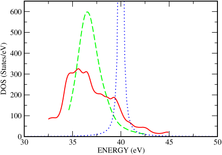
Figure 1: (Color online) Atomic spectrum of eigenvalues of Pu without spin-orbit coupling, with N=5 electrons for single U (dotted line), density-density approximation (dashed line) and spin-flip terms (full line) included respectively.

III.2 Results

In Figs. 1 and 2, the density of states (DOS) is the sum of all Lorentzians from each eigenvalue. We note that this DOS should not be confused with the spectral density presented in next part: it is just a visual way of presenting the distribution of eigenvalues. For illustration, we present the case of plutonium where the Slater integrals parameters are given in Table I. Figure 1 presents the atomic spectrum of eigenvalues of Pu without spin-orbit coupling, for a given occupancy of $N=5$ electrons. The different approximations with increasing order of complexity are displayed: single $U$, density-density approximation and spin-flip terms included respectively. Figure 2 displays the same situation when spin-orbit coupling has been taken into account for occupancies of $N=5$ and $N=6$ electrons.

The most accurate description is given when the spin-flip terms are not neglected. In this case, the spectrum is much more structured than the result for the density-density approximation. The spin-flip terms in the Hamiltonian couple different states that are degenerate in the density-density approximation, and split them. This causes the additional structure in the spectrum. The density-density approximation spectrum therefore has less structure, but has its gross features centered in the same region as the spectrum which include the spin-flips. For the single $U$ limit result, for a given occupancy $N$ and neglecting of spin-orbit coupling, there is a single eigenvalue $U{N(N-1)}/{2}$ whose degeneracy equals the dimension of subspace. This is the origin, when smeared with a Lorentzian, of the single peak, which is actually too high in energy and well separated from the more realistic spectrum in the density-density approximation or the one including spin-flip terms (roughly 5 eV above the center of gravity of the other ones). Clearly, the single $U$ limit overestimates the interaction energy. This is mainly caused by the complete neglect of any exchange term, which would reduce the average interaction. This approximation, which has been widely used, can be a problem for an atom embedded in a solid, since the metal-insulator transition is a delicate balance between localization due to the interaction $U$ and delocalization, represented by a bandwidth W. Thus the single $U$ limit could artificially push the system towards an insulating state, or at least, increases the localized characters of the $f$-electrons. To remedy this situation, without increasing the level of complexity of the solution, would be to replace the single $U$ limit by a single $U-J$, since we have seen above that there is always an exchange term in the density-density approximation for the $jm_{j}$ basis. In that case, taking the overall average exchange $\overline{J}=0.323eV$ of Eq. (25), one would obtain a single peak located at 36.77 eV, which is in better agreement with more elaborated results, and especially very close to the central maximum of the density-density result.

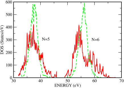
Figure 2: (Color online) Atomic spectrum of eigenvalues of Pu with spin-orbit coupling, with N=5 and N=6 electrons for density-density approximation (dashed line) and spin-flip terms included (full line) respectively.

IV Atomic Temperature Green’s function

As mentioned in the introduction, one cannot neglect a correct description of the atomic aspects of strongly correlated electrons systems. In this part we concentrate on the atomic (i.e., local) Green’s function of an atom, which will be later embedded in a solid. The results presented in this section can be seen as a first step, with further hybridization to the rest of the medium to be be added later as, for example, is done in the DMFT approach. We start from the definition of (imaginary time) temperature Green function :

$$\mathcal{G}_{k}(\tau)=-\langle T_{\tau}c_{k}(\tau)c_{k}^{\dagger}(0)\rangle\;,$$ (29)

where $c_{k}^{\dagger}$ is a creation operator in a state $k$, which is, in the present case, one of the 14 atomic orbitals of the $jm_{j}$ basis for $\ell=3$. Based on the antiperiodic property

$$\mathcal{G}_{k}(\tau+\beta)=-\mathcal{G}_{k}(\tau)\;,$$ (30)

where ${1}/{\beta}$ is the temperature, one can write the Fourier expansion of $\mathcal{G}_{k}(\tau)$ as

$$\mathcal{G}_{k}(\tau)=\frac{1}{\beta}\sum_{i\omega_{n}}e^{-i\omega_{n}\tau}\mathcal{G_{k}}(i\omega_{n})\;,$$ (31)

with the Fourier transform

$$\mathcal{G}_{k}(i\omega_{n})=\int_{0}^{\beta}e^{i\omega_{n}\tau}\mathcal{G}_{k}(\tau)d\tau\;.$$ (32)

The Matsubara frequencies $\omega_{n}$ are given by:

$$\omega_{n}=(2n+1)\pi/\beta\;.$$ (33)

If the eigenstates $|a\rangle$ and their eigenvalue $E_{a}$ are known from a diagonalization of the Hamiltonian, then Eq. (32) has the following Lehmann representation:

$$\mathcal{G}_{k}(i\omega_{n})=\frac{1}{Z_{G}}\sum_{a,b}|\langle a|c_{k}|b\rangle|^{2}\frac{e^{-\beta E^{\prime}_{a}}+e^{-\beta E^{\prime}_{b}}}{i\omega_{n}+E^{\prime}_{a}-E^{\prime}_{b}}\;.$$ (34)

Here $Z_{G}$ is the grand partition function:

$$Z_{G}=Tre^{-\beta(H-\mu N)}\;,$$ (35)

$E^{\prime}_{a}=E_{a}-\mu N_{a}$, and $\mu$, the chemical potential, is chosen to fix the average number of particles with:

$$\sum_{k}\frac{1}{\beta}\sum_{i\omega_{n}}e^{+i\omega_{n}0^{+}}\mathcal{G}_{k}(i\omega_{n})=\sum_{k}N_{k}\;.$$ (36)

Eq. (34) can be used to define the spectral density; this can be compared to photoemission experiments, and is given by

$$\rho_{k}(\omega)=\frac{1}{Z_{G}}\sum_{a,b}|\langle a|c_{k}|b\rangle|^{2}(e^{-\beta E^{\prime}_{a}}+e^{-\beta E^{\prime}_{b}})\delta(\omega+E^{\prime}_{a}-E^{\prime}_{b})\;.$$ (37)

Because the sum involves discrete eigenstates for the atomic case, we add to $\omega$ a small imaginary part so that the spectral density becomes a sum of Lorentzians when the results are presented. It should also be noted that for solids the atomic Green’s function tends to become a very good approximation at sufficiently high temperature (see, for example, the discussion of Fig. 2 in Ref. AMcMahan, ).

IV.1 Comparison of the single $U$ model with the density-density approximation

Since all states of a given occupancy $N$ are degenerate with eigenenergy $U{N(N-1)}/{2}$ when spin-orbit is neglected, the single $U$ model has an analytical expression for the Green function, which can be written:

$$\mathcal{G}_{k}(i\omega_{n}) =\frac{1}{Z_{G}}\sum_{N}\frac{13!}{N!(13-N)!}$$

$$\times\frac{e^{-\beta N[\frac{N-1}{2}U-\mu]}+e^{-\beta(N+1)[\frac{N}{2}U-\mu]}}{i\omega_{n}+\mu-NU}\;.$$ (38)

This result, which can be presented in a form previously obtained by McMahan et al., AMcMahan shows evenly spaced values separated by $U$ in the poles of the Green function.

When spin-orbit is switched on ($\chi\neq 0$), it is less convenient to give an simple analytical formula, since the degeneracy of the states is partially lifted. We present the spectral density for this case in Fig. 3. One can still see the effect of approximately evenly spaced values of the order of $U$ for the poles, but additional structure also appears. Note that the effect of temperature, here chosen to be 15800 K, allows additional excited states to appear in the spectra. A lower temperature would have completely quenched much of this additional structure. In addition, this temperature has been used in some recent DMFT Pu calculations to check the Quantum Monte Carlo (QMC) DMFT codes against atomic-like Hubbard-I approximations Zhu07 , since the atomic limit is a good approximation at this temperature. The average $f$-occupancy is chosen to be about 5.6 in accordance with the result of Ref Zhu07 . The comparison with the density-density approximation spectral density (dashed line) in Fig. 3 clearly shows that the single $U$ approximation is an oversimplified model for the correlation effects, and misses many of the features of even the density-density results, and misplaces some of the peaks.

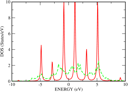
Figure 3: (Color online) Spectral density of atomic Pu at T=15800K, for single U limit (full line) and density-density approximation (dashed line) respectively, including spin-orbit coupling in both cases.

IV.2 Comparison of the density-density approximation with exact results

In Fig. 4 we show the exact results for the spectral density (within the basis we have chosen). These include the spin-flip terms and involve exact diagonalization of the local atomic Hamiltonian. In this figure we also include the decomposition of the spectra into its 5/2 and 7/2 contributions, with their respective weights of 6 and 8. As expected, the spin-orbit splitting has displaced the gross features of the 5/2 density downward with respect to those of the 7/2 features. These spectral densities have much more structure in them than the density-density result.

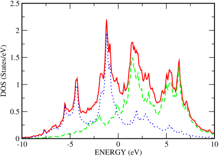
Figure 4: (Color online) Exact results, which include spin-flip terms in Hamiltonian, for the total (full line), and 5/2 (dotted line) and 7/2 (dashed line) projected spectral densities of atomic Pu at T=15800K, including spin-flip terms in Hamiltonian

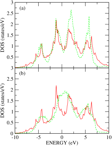
Figure 5: (Color online) Comparison of the spectral density of atomic Pu, including spin-flip terms in Hamiltonian (full line), with the density-density approximation result (dashed line). The upper panel (a) provides results for the density-density approximation for j-j coupling ($n_{j}n_{j^{\prime}}$) whereas the bottom panel (b) is for the case of $ls$ coupling ($n_{ls}n_{l^{\prime}s^{\prime}}$). Note that for the latter case the full matrix must be diagonalized since the spin-orbit coupling term is not diagonal in the $ls$ basis. The spin-flip case is reproduced in both panels for comparison.

In Fig. 5 we compare the spectral density for the density-density approximation with the exact results for both $j$-$j$ and $ls$ coupling. Both show a similar overall gross structure of the spectrum, which is located in approximately the same energy range. However, the $j$-$j$ coupling clearly does a much superior job in reproducing the actual peak structure in the spectrum. In addition, the excellent agreement between the $j$-$j$ density-density approximation and exact spectral densities suggests that in many situations the $j$-$j$ density-density approximation may be an adequate approximation to more refined treatments of the Coulomb effects for Pu. It is worth mentioning that, when all terms are retained as here, i.e., spin-orbit and full electrostatic interaction, the results do not depend on the basis chosen for the representation; the local Hamiltonian that would have been solved from the $LS$ basis would have had the same final spectral density. Thus the similarity we stress between the full result and the density-density approximation is not an artifact of the choice of representation, namely the $jm_{j}$ basis.

V Summary and conclusion

We have presented a study of the atomic electronic structure of the $f$-electron elements in the presence of spin-orbit coupling, and applied this to plutonium. We have emphasized the role of electronic interactions in a $jm_{j}$ basis. For this purpose, we have derived a general analytical expression for the matrix elements of the interaction in this basis; some of these that can be used in a density-density approximation have been tabulated, since they could be useful for possible calculations in solids. We have used these to study the effect of Coulomb interactions on the eigenvalue and spectral functions. Diagonalizations of this Hamiltonian for different occupancies and computations of spectral density, have been performed in various approximations, including single $U$, single $U-J$, density-density ,and, finally, the full interaction matrix retaining all spin-flip terms. We have found that the density-density approximation, in the $jm_{j}$ basis, which neglects off-diagonal terms (i.e., spin-flip terms) in the interaction matrix, gives excellent agreement with the full interaction.

The high accuracy of the $j$-$j$ density-density approximation should make it very useful in electronic-structure calculations for solids. For example, it is a very tractable method for the Hirsch-Fye algorithm of the QMC solver in DMFT, and should makes the application of the Gutzwiller method much easier.

VI Acknowledgments

This work was carried out under the auspices of the National Nuclear Security Administration of the U.S. Department of Energy at Los Alamos National Laboratory under Contract No. DE-AC52-06NA25396. Financial supports from LANL Theoretical Division (CNLS and T-11 group) as well as DGA (Delegation Generale pour l’Armement Contract No. 07.60.028.00.470.75.01) are gratefully acknowledged. J.-P. J also acknowledges the LANL group for his warm hospitality during his stay in Los Alamos, USA.

*

Appendix A Expression of the general matrix element in the $jm_{j}$ basis

We demonstrate now formula (11). The general expression element of the Coulomb interaction in $jm_{j}$ basis is $V_{1234}=\langle j_{1}M_{1}j_{2}M_{2}|V|j_{3}M_{3}j_{4}M_{4}\rangle$. In this appendix to avoid too heavy notations, we will use the notation $|jM\rangle$ for an element of the $jm_{j}$ basis and $|\ell m\sigma\rangle$ to designate the state $|\ell\,m_{\ell}\,s\,m_{s}\rangle$ of the $\ell m_{\ell}$ basis. $j_{1}$ to $j_{4}$ could be one of either $\ell+\frac{1}{2}$ or $\ell-\frac{1}{2}$ total momentum quantum number ($\ell$ being well defined here). By inserting four times the Clebsch-Gordan (CG) expansion:

$$|jM\rangle=\sum_{m\sigma}|\ell m\sigma\rangle\langle\ell m\sigma|jM\rangle$$ (39)

in the definition of $V_{1234}$, where $\langle\ell m\sigma|jM\rangle$ is a shorthand for the (chosen real) CG coefficient $\langle\ell m\frac{1}{2}\sigma|(\ell\frac{1}{2})jM\rangle$, one obtains:

$$V_{1234} = \sum_{m_{1}\sigma_{1}m_{2}\sigma_{2}m_{3}\sigma_{3}m_{4}\sigma_{4}}\langle\ell m_{1}\sigma_{1}|j_{1}M_{1}\rangle\langle\ell m_{2}\sigma_{2}|j_{2}M_{2}\rangle$$

$$\times\langle\ell m_{3}\sigma_{3}|j_{3}M_{3}\rangle\langle\ell m_{4}\sigma_{4}|j_{4}M_{4}\rangle$$

$$\times\langle\ell m_{1}\sigma_{1}\,\ell m_{2}\sigma_{2}|V|\ell m_{3}\sigma_{3}\,\ell m_{4}\sigma_{4}\rangle\;.$$

(40)

The matrix element of interaction in the $\ell m_{\ell}$ basis appearing in this last formula can be expressed as:

$$\langle\ell m_{1}\sigma_{1} \ell m_{2}\sigma_{2}|V|\ell m_{3}\sigma_{3}\ell m_{4}\sigma_{4}\rangle=\delta_{\sigma_{1}\sigma_{3}}\delta_{\sigma_{2}\sigma_{4}}$$

$$\times\int drd\Omega dr^{\prime}d\Omega^{\prime}Y_{\ell m_{1}}^{*}(\Omega)Y_{\ell m_{2}}^{*}(\Omega^{\prime})$$

$$\times|R_{n\ell}(r)|^{2}\frac{1}{|r-r^{\prime}|}|R_{n\ell}(r^{\prime})|^{2}Y_{\ell m_{3}}(\Omega)Y_{\ell m_{4}}(\Omega^{\prime})\;.$$

¿From Eq. (8), the above integral can be conveniently cast into a sum of a product of one radial integral (identified as the Slater integral (13)) and two angular integrals:

$$\sum_{k=0}^{\infty}\sum_{q=-k}^{k} \frac{4\pi}{2k+1}\int drdr^{\prime}|R_{n\ell}(r)|^{2}\frac{r_{<}^{k}}{r_{>}^{k+1}}|R_{n\ell}(r^{\prime})|^{2}$$

$$\times\int d\Omega Y_{\ell m_{1}}^{*}(\Omega)Y_{kq}^{*}(\Omega)Y_{\ell m_{3}}(\Omega)$$

$$\times\int d\Omega^{\prime}Y_{\ell m_{2}}^{*}(\Omega^{\prime})Y_{kq}(\Omega^{\prime})Y_{\ell m_{4}}(\Omega^{\prime})\;.$$ (42)

With conjugation relation $Y_{\ell m}^{*}(\Omega)=(-)^{m}Y_{\ell-m}(\Omega)$, each one of the two angular integrals can calculated from a well-known identity giving the integral of the product of three spherical harmonics:

$$\int d\Omega Y_{\ell_{1}m_{1}} (\Omega)Y_{\ell_{2}m_{2}}(\Omega)Y_{\ell_{3}m_{3}}(\Omega)=(-)^{m_{3}}$$

$$\times\sqrt{\frac{(2\ell_{1}+1)(2\ell_{2}+1)}{4\pi(2\ell_{3}+1)}}$$

$$\times\langle\ell_{1}0\ell_{2}0|\ell_{3}0\rangle\langle\ell_{1}m_{1}\ell_{2}m_{2}|\ell_{3}\,{-}m_{3}\rangle\;.$$ (43)

Application of this last identity with the selection rule for CG coefficients $\langle\ell_{1}m_{1}\ell_{2}m_{2}|\ell_{3}m_{3}\rangle$ which vanish unless $m_{3}=m_{1}+m_{2}$, enables to rewrite (LABEL:A3):

$$\langle\ell m_{1} \sigma_{1}\,\ell m_{2}\sigma_{2}|V|\ell m_{3}\sigma_{3}\,\ell m_{4}\sigma_{4}\rangle=(-)^{m_{1}-m_{2}}$$

$$\times\delta_{\sigma_{1}\sigma_{3}}\delta_{\sigma_{2}\sigma_{4}}\delta_{m_{1}+m_{2},m_{3}+m_{4}}\sum_{k=0}^{2\ell}F^{(k)}\frac{(2\ell+1)^{2}}{(2k+1)^{2}}$$

$$\times\langle\ell\,0\,\ell\,0|k\,0\rangle^{2}\langle\ell\,{-}m_{1}\,\ell\,m_{3}|k\,m_{3}{-}m_{1}\rangle$$

$$\times\langle\ell\,{-}m_{2}\,\ell\,m_{4}|k\,m_{4}{-}m_{2}\rangle\;.$$ (44)

The fact that CG $\langle\ell\;0\;\ell\;0|k\;0\rangle$ vanishes unless $2\ell+k$ is even and $k$ preserves the well-known triangle condition, namely $0\leq k\leq 2\ell$, enables to restrain summation to even values of $k$ from 0 to $2\ell$, i.e. limited to $k=6$ for $f$ states, requiring only Slater integrals $F^{(0)}$ to $F^{(6)}$, given in Table I for Plutonium. Replacement of result (44) into expression (40), associated with selection rule for CG coefficients $\langle\ell\;m\;\sigma|j\;M\rangle$ which vanish unless $M=m+\sigma$, and final use of identity for $\pm\frac{1}{2}$ spins, $(-)^{\sigma_{1}-\sigma_{2}}=(2\sigma_{1})(2\sigma_{2})$, one derives directly expression:

$$V_{1234} =\delta_{M_{1}+M_{2},M_{3}+M_{4}}(-)^{(M_{3}-M_{2})}$$

$$\times\sum_{k=0}^{2\ell}F^{(k)}\frac{(2\ell+1)^{2}}{(2k+1)^{2}}\langle\ell\,0\,\ell\,0|k\,0\rangle^{2}$$

$$\times\sum_{\sigma_{1}\sigma_{2}}(2\sigma_{1})(2\sigma_{2})\langle\ell\,M_{1}{-}\sigma_{1}\,\sigma_{1}|j_{1}\,M_{1}\rangle$$

$$\times\langle\ell\,M_{2}{-}\sigma_{2}\,\sigma_{2}|j_{2}\,M_{2}\rangle\langle\ell\,M_{3}{-}\sigma_{1}\,\sigma_{1}|j_{3}\,M_{3}\rangle$$

$$\times\langle\ell\,M_{4}{-}\sigma_{2}\,\sigma_{2}|j_{4}\,M_{4}\rangle$$

$$\times\langle\ell\,{-}(M_{1}{-}\sigma_{1})\,\ell,M_{3}{-}\sigma_{1}|k\,M_{3}{-}M_{1}\rangle$$

$$\times\langle\ell\,{-}(M_{2}{-}\sigma_{2})\,\ell\,M_{4}{-}\sigma_{2}|k\,M_{4}{-}M_{2}\rangle\;,$$ (45)

from which one obtains expression (11) when we make an identification of definition (12) for auxiliary function $B_{k}^{\ell}(jm;j^{\prime}m^{\prime})$.

Application of formula (11) to direct and exchange cases lead us to arrive at Eqs. (LABEL:aso) and (17), respectively. From these expressions and the CG related symmetries properties of function $B_{k}^{\ell}(jm;j^{\prime}m^{\prime})$ given in (12), one can give the symmetry relations that $a$ and $b$’s obey, reducing the number entries of Tables II and III. The matrix elements not given in those Tables can be consequently obtained using the following symmetries:

$$a_{k}^{\ell}(j,|m|;j^{\prime},|m^{\prime}|) = a_{k}^{\ell}(jm;j^{\prime}m^{\prime})\;,$$ (46)

and

$$b_{k}^{\ell}(jm;j^{\prime}m^{\prime}) = b_{k}^{\ell}(j\,{-}m;j^{\prime}\,{-}m^{\prime})\;,$$

$$b_{k}^{\ell}(j\,{-}m;j^{\prime},m^{\prime}) = b_{k}^{\ell}(j,m;j^{\prime}\,{-}m^{\prime})\;.$$ (47)

Table 2: Values of $a_{k}^{\ell}(jm;j^{\prime}m^{\prime})$ for the direct interaction matrix element $\langle jmj^{\prime}m^{\prime}|V|jmj^{\prime}m^{\prime}\rangle=\sum_{k}a_{k}^{\ell}(jm;j^{\prime}m^{\prime})F^{(k)}$ for $\ell=3$ in the $jm_{j}$ basis.

$j$	$|m_{j}|$	$j^{\prime}$	$|m_{j}^{\prime}|$	$F^{(2)}$	$F^{(4)}$	$F^{(6)}$
7/2	7/2	7/2	7/2	49/441	49/5929	25/184041
	7/2		5/2	7	-91	-125
	7/2		3/2	-21	-21	225
	7/2		1/2	-35	63	-125
	5/2		5/2	1	169	625
	5/2		3/2	-3	39	-1125
	5/2		1/2	-5	-117	625
	3/2		3/2	9	9	2025
	3/2		1/2	15	-27	-1125
	1/2		1/2	25	81	625
7/2	7/2	5/2	5/2	70/735	7/1617	0
	7/2		3/2	-14	-21	0
	7/2		1/2	-56	14	0
	5/2		5/2	10	-13	0
	5/2		3/2	-2	39	0
	5/2		1/2	-8	-26	0
	3/2		5/2	-30	-3	0
	3/2		3/2	6	9	0
	3/2		1/2	24	-6	0
	1/2		5/2	-50	9	0
	1/2		3/2	10	-27	0
	1/2		1/2	40	54	0
5/2	5/2	5/2	5/2	100/ 1225	1/441	0
	5/2		3/2	-20	-3	0
	5/2		1/2	-80	2	0
	3/2		3/2	4	9	0
	3/2		1/2	16	-6	0
	1/2		1/2	64	4	0

Table 3: Values of $b_{k}^{\ell}(jm;j^{\prime}m^{\prime})$ for the exchange interaction matrix element $\langle jmj^{\prime}m^{\prime}|V|j^{\prime}m^{\prime}jm\rangle=\sum_{k}b_{k}^{\ell}(jm;j^{\prime}m^{\prime})F^{(k)}$ for $\ell=3$ in the $jm_{j}$ basis.

$j$	$m_{j}$	$j^{\prime}$	$m_{j}^{\prime}$	$F^{(2)}$	$F^{(4)}$	$F^{(6)}$
7/2	$\pm 7/2$	7/2	$\pm 7/2$	49/441	49/5929	25/184041
	$\pm 7/2$		$\pm 5/2$	42	140	150
	$\pm 7/2$		$\pm 3/2$	14	210	500
	$\pm 7/2$		$\pm 1/2$	0	196	1200
	$\pm 7/2$		$\mp 1/2$	0	98	2250
	$\pm 7/2$		$\mp 3/2$	0	0	3300
	$\pm 7/2$		$\mp 5/2$	0	0	3300
	$\pm 7/2$		$\mp 7/2$	0	0	0
	$\pm 5/2$		$\pm 5/2$	1	169	625
	$\pm 5/2$		$\pm 3/2$	32	60	1400
	$\pm 5/2$		$\pm 1/2$	30	2	2100
	$\pm 5/2$		$\mp 1/2$	0	112	2100
	$\pm 5/2$		$\mp 3/2$	0	210	1050
	$\pm 5/2$		$\mp 5/2$	0	0	0
	$\pm 3/2$		$\pm 3/2$	9	9	2025
	$\pm 3/2$		$\pm 1/2$	60	108	1750
	$\pm 3/2$		$\mp 1/2$	40	96	700
	$\pm 3/2$		$\mp 3/2$	0	0	0
	$\pm 1/2$		$\pm 1/2$	25	81	625
	$\pm 1/2$		$\mp 1/2$	0	0	0
7/2	$\pm 7/2$	5/2	$\pm 5/2$	175/11025	210/53361	25/184041
	$\pm 7/2$		$\pm 3/2$	140	756	200
	$\pm 7/2$		$\pm 1/2$	0	1323	900
	$\pm 7/2$		$\mp 1/2$	0	1176	3000
	$\pm 7/2$		$\mp 3/2$	0	0	8250
	$\pm 7/2$		$\mp 5/2$	0	0	19800
	$\pm 5/2$		$\pm 5/2$	150	600	150
	$\pm 5/2$		$\pm 3/2$	5	1014	875
	$\pm 5/2$		$\pm 1/2$	160	486	2800
	$\pm 5/2$		$\mp 1/2$	0	21	6300
	$\pm 5/2$		$\mp 3/2$	0	1344	10500
	$\pm 5/2$		$\mp 5/2$	0	0	11550
	$\pm 3/2$		$\pm 5/2$	75	1000	525
	$\pm 3/2$		$\pm 3/2$	90	640	2250
	$\pm 3/2$		$\pm 1/2$	30	1	5250
	$\pm 3/2$		$\mp 1/2$	120	578	8400
	$\pm 3/2$		$\mp 3/2$	0	686	9450
	$\pm 5/2$		$\mp 5/2$	0	560	6300
	$\pm 1/2$		$\pm 5/2$	20	1200	1400
	$\pm 1/2$		$\pm 3/2$	121	120	4375
	$\pm 1/2$		$\pm 1/2$	12	300	7500
	$\pm 1/2$		$\mp 1/2$	98	735	8750
	$\pm 1/2$		$\mp 3/2$	64	60	7000
	$\pm 1/2$		$\mp 5/2$	0	1050	3150
5/2	$\pm 5/2$	5/2	$\pm 5/2$	100/1225	1/441	0
	$\pm 5/2$		$\pm 3/2$	120	4	0
	$\pm 5/2$		$\pm 1/2$	60	9	0
	$\pm 5/2$		$\mp 1/2$	0	14	0
	$\pm 5/2$		$\mp 3/2$	0	14	0
	$\pm 5/2$		$\mp 5/2$	0	0	0
	$\pm 3/2$		$\pm 3/2$	4	9	0
	$\pm 3/2$		$\pm 1/2$	48	10	0
	$\pm 3/2$		$\mp 1/2$	108	5	0
	$\pm 3/2$		$\mp 3/2$	0	0	0
	$\pm 1/2$		$\pm 1/2$	64	4	0
	$\pm 1/2$		$\mp 1/2$	0	0	0

References

- (1) P. Hohenberg et W. Kohn, Phys. Rev. 136, 864 (1964).
- (2) W. Kohn et L. J. Sham, Phys. Rev. 140, 1133(1965).
- (3) V. I. Anisimov, J. Zaanen, et O. K. Andersen, Phys. Rev. B 44, 943 (1991).
- (4) J. Bouchet, S. Siberchicot, A. Pasturel and F. Jollet, J. Phys.: Condens. Matter 12, 1723 (2000).
- (5) A. Georges, G. Kotliar, W. Krauth, and J. Rozenberg, Rev. Mod. Phys. 68, 13 (1996).
- (6) V. I. Anisimov, A. I. Poteryaev, M. A. Korotin, A. O. Anokhin, and G. Kotliar, J. Phys.: Condens. Matter 9, 7359 (1997).
- (7) S.Y. Savrasov and G. Kotliar, Phys. Rev. Lett. 84, 3670 (2000).
- (8) M.C. Gutzwiller, Phys. Rev. Lett. 10, 159 (1963).
- (9) A. I. Liechtenstein, V. I. Anismov, J. Zaanen, Phys. Rev. B 52, R5467(1995).
- (10) J. Bünemann, W. Weber and F. Gebhard, Phys. Rev. B 57, 6896 (1998).
- (11) G. Kotliar and A.R. Ruckenstein, Phys. Rev. Lett. 57, 1362 (1986).
- (12) F. Lechermann, A. Georges, G. Kotliar and O. Parcollet, cond-mat/0704.1434v1 (2007).
- (13) J.-P. Julien and J. Bouchet, Prog. Theor. Chem. Phys. B 15, 509 (2006).
- (14) D. R. Inglis, Phys. Rev. 38, 862(1931).
- (15) E. U. Condon and G. H. Shortley, The Theory of Atomic Spectra, Cambridge University Press, third edition (1963).
- (16) V.I. Anisimov, O. Gunnarsson, Phys. Rev. B 43, 7570(1991).
- (17) M.T. Czyżyk, and G.A. Sawatzky, Phys. Rev. B 49, 14211(1994). V.I. Anisimov, I.V. Solovyev, M. A. Korotin, M.T. Czyżyk, and G.A. Sawatzky, Phys. Rev. B 48, 16929(1993).
- (18) J. E. Hirsch and R. M. Fye, Phys. Rev. Lett. 56, 2521 (1986).
- (19) A.K. McMahan, K. Held, and R.T. Scalettar, Phys. Rev. B 67, 075108(2003).
- (20) A. Shick, J. Kolorenc, L. Havela, V. Drchal and T. Gouder, cond-mat/0610794 (2006).
- (21) A. Hjelm, J. Trygg, O. Eriksson, B. Johansson and J. Wills, Phys. Rev. B 50, 4332 (1994).
- (22) J.-X. Zhu et al., arXiv:0705.1354 (2007),to appear in Phys. Rev. B.
*