Luminosity Dependent X-ray AGN Clustering ?

Abstract

We have analysed the angular clustering of X-ray selected active galactic nuclei (AGN) in different flux-limited sub-samples of the Chandra Deep Field North (CDF-N) and South (CDF-S) surveys. We find a strong dependence of the clustering strength on the sub-sample flux-limit, a fact which explains most of the disparate clustering results of different XMM and Chandra surveys. Using Limber’s equation, we find that the inverted CDF-N and CDF-S spatial clustering lengths are consistent with direct spatial clustering measures found in the literature, while at higher flux-limits the clustering length increases considerably; for example, at $f_{x,{\rm limit}}\sim 10^{-15}$ erg s^-1 cm^-2 we obtain $r_{0}\simeq 17\pm 5$ and $18\pm 3\;h^{-1}$ Mpc, for the CDF-N and CDF-S, respectively. We show that the observed flux-limit clustering trend hints towards an X-ray luminosity dependent clustering of X-ray selected, $z\sim 1$, AGNs.

1 Introduction

X-ray selected AGNs provide a relatively unbiased census of the AGN phenomenon, since obscured AGNs, largely missed in optical surveys, are included in such surveys. Furthermore, they can be detected out to high redshifts and thus trace the distant density fluctuations providing important constraints on supermassive black hole formation, the relation between AGN activity and Dark Matter (DM) halo hosts, the cosmic evolution of the AGN phenomenon (eg. Mo & White 1996, Sheth et al. 2001), and on cosmological parameters and the dark-energy equation of state (eg. Basilakos & Plionis 2005; 2006, Plionis & Basilakos 2007).

Until quite recently our knowledge of X-ray AGN clustering came exclusively from analyses of ROSAT data ($\leq 3$keV) (eg. Boyle & Mo 1993; Vikhlinin & Forman 1995; Carrera et al. 1998; Akylas, Georgantopoulos, Plionis, 2000; Mullis et al. 2004). These analyses provided conflicting results on the nature of high-$z$ AGN clustering. Vikhlinin & Forman (1995), using the angular correlation approach and inverting to infer the spatial correlation length, found a strong amplitude of $\bar{z}\sim 1$ sources ($r_{0}\simeq 9\;h^{-1}$ Mpc), which translates into $r_{0}\simeq 12\;h^{-1}$ Mpc for a $\Lambda$CDM cosmology and a luminosity driven density evolution (LDDE) luminosity function (eg. Hasinger et al. 2005). Carrera et al. (1998), however, using spectroscopic data, could not confirm such a large correlation amplitude.

With the advent of the XMM and Chandra X-ray observatories, many groups have attempted to settle this issue. Recent determinations of the high-$z$ X-ray selected AGN clustering, in the soft and hard bands, have provided again a multitude of conflicting results, intensifying the debate (eg. Yang et al. 2003; Manners et al. 2003; Basilakos et al. 2004; Gilli et al. 2005; Basilakos et al 2005; Yang et al. 2006; Puccetti et al. 2006; Miyaji et al. 2007; Gandhi et al. 2006; Carrera et al. 2007).

In this letter we investigate these clustering differences by re-analysing the CDF-N and CDF-S surveys, using the Bauer et al. (2004) classification to select only AGNs in the 0.5-2 and 2-8 keV bands. To use all the available sources, and not only those having spectroscopic redshifts, we work in angular space and then invert the angular correlation function using Limber’s equation. Hereafter, we will be using $h\equiv H_{\circ}/100$ km $s^{-1}$ Mpc^-1.

2 The X-ray source catalogues

The 2Ms CDF-N and 1Ms CDF-S Chandra data represent the deepest observations currently available at X-ray wavelengths (Alexander et al. 2003, Giaconni et al. 2001). The CDF-N and CDF-S cover an area of 448 and 391 arcmin², respectively. We use the source catalogues of Alexander et al. (2003) for both CDF-N and CDF-S. The flux limits that we use for the CDF-N are $3\times 10^{-17}$ and $2\times 10^{-16}$ $\rm erg~{}cm^{-2}~{}s^{-1}$ in the soft and hard band, while for the CDF-S the respective values are $6\times 10^{-17}$ and $5\times 10^{-16}$ erg cm^-2 s^-1. Note that sensitivity maps were produced following the prescription of Lehmer et al. (2005) and in order to produce random catalogues in a consistent manner to the source selection, we discard sources which lie below our newly determined sensitivity map threshold, at their given position. Our final CDF-N catalogues contain 383 and 263 sources in the soft (0.5-2 keV) and hard band (2-8 keV), respectively, out of which 304 and 255 are AGNs, according to the “pessimistic” Bauer et al. (2004) classification. The corresponding CDF-S catalogues contain 257 and 168 sources in the same bands, out of which 227 and 165 are AGNs. A number of sources (roughly half) have spectroscopic redshift determinations (mostly taken from Barger et al. 2003; Szokoly et al. 2004; Vanzella et al. 2005; Vanzella et al. 2006; Le Févre et al. 2004; Mignoli et al. 2005).

3 Correlation function analysis

3.1 The angular correlation

The clustering properties of the X-ray AGNs are estimated using the two-point angular correlation function, $w(\theta)$, estimated using $w(\theta)=f(N_{DD}/N_{DR})-1$, where $N_{DD}$ and $N_{DR}$ is the number of data-data and data-random pairs, respectively, within separations $\theta$ and $\theta+d\theta$. The normalization factor is given by $f=2N_{R}/(N_{D}-1)$, where $N_{D}$ and $N_{R}$ are the total number of data and random points respectively. The Poisson uncertainty in $w(\theta)$ is estimated as $\sigma_{w}=\sqrt{(1+w(\theta))/N_{DR}}$ (Peebles 1973).

The random catalogues are produced to account for the different positional sensitivity and edge effects of the surveys. To this end we generated 1000 Monte Carlo random realizations of the source distribution, within the CDF-N and CDF-S survey areas, by taking into account the local variations in sensitivity. We also reproduce the desired $\log N-\log S$ distribution, either the Kim et al. (2007) or the one recovered directly from the CDF data (however our results remain mostly unchanged using either of the two). Random positioned sources with fluxes lower than that corresponding to the particular position of the sensitivity map are removed from our final random catalogue.

We apply the correlation analysis evaluating $w(\theta)$ in the range $[5^{{}^{\prime\prime}},900^{{}^{\prime\prime}}]$ in 10 logarithmic intervals with $\delta\log\theta=0.226$. We find statistically significant signals for all bands and for both CDF-N and CDF-S. As an example we provide in Table 1 the integrated signal to noise ratios, given for two different flux-limits and two different angular ranges. The significance appears to be low only for the CDF-S hard-band, but for the lowest flux-limit.

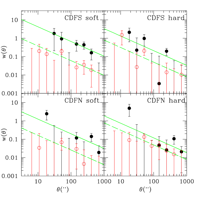
Figure 1: The CDF-S and CDF-N angular correlation function. The open points correspond to the overall sample, while the filled points to the highest flux-limit used ($f_{x}=3\times 10^{-15}$ ${\rm erg/s/cm^{2}}$ for the soft and $f_{x}=5\times 10^{-15}$ ${\rm erg/s/cm^{2}}$ for the hard bands, respectively). The straight lines correspond to the best power-law fit to the clustering data. Errorbars correspond to $1\sigma$ Poisson uncertainties.

The angular correlation function for two different flux-limits are shown in Figure 1, with the lines corresponding to the best-fit power law model: $w(\theta)=(\theta_{0}/\theta)^{\gamma-1}$, using $\gamma=1.8$ and the standard $\chi^{2}$ minimization procedure. Note that for the CDF-N, we get at some $\theta$’s very low or negative $w(\theta)$ values. These, however, are taken into account in deriving the integrated signal, presented in Table 1.

Applying our analysis for different flux-limited sub-samples, we find that the clustering strength increases with increasing flux-limit, in agreement with the CDF-S results of Giacconi et al (2001). In Figure 2 we plot the angular clustering scale, $\theta_{0}$, derived from the power-law fit of $w(\theta)$, as a function of different sample flux-limits. The trend is true for both energy bands and for both CDF-N and CDF-S, although for the latter is apparently stronger.

We also find that at their lowest respective flux-limits the clustering of CDF-S sources is stronger than that of CDF-N (more so for the soft-band), in agreement with the spatial clustering analysis of Gilli et al. (2005). This difference has been attributed to cosmic variance, in the sense that there are a few large superclusters present in the CDF-S (Gilli et al. 2003). However, selecting CDF-N and CDF-S sources at the same flux-limit reduces this difference, which remains strong only for the highest flux-limited sub-samples (see Fig.2).

It is worth mentioning that our results could in principle suffer from the so-called amplification bias, which can enhance artificially the clustering signal due to the detector’s PSF smoothing of source pairs with intrinsically small angular separations (see Vikhlinin & Forman 1995; Basilakos et al. 2005). However, we doubt whether this bias can significantly affect our results because at the median redshift of the sources ($z\sim 1$) the Chandra PSF angular size of $\sim 1^{{}^{\prime\prime}}$ corresponds to a rest-frame spatial scale of only $\sim 5$ $h^{-1}$ kpc (even at large off-axis angles, where the PSF size increases to $\sim 4^{{}^{\prime\prime}}$, the corresponding spatial scale is only $\sim 20$ $h^{-1}$ kpc). In any case, and ignoring for the moment the additional effect of the variable PSF size, the above imply that only the $w(\theta)$ of the lowest flux-limited samples could in principle be affected, but in the direction of reducing (and not inducing) the observed $\theta_{0}-f_{x,{\rm limit}}$ trend (since the uncorrected $\theta_{0}$ values are, if anything, artificially larger than the true underlying one).

However, the variability of the PSF size through-out the Chandra field can have an additional effect, and possibly enhance or even produce the observed $\theta_{0}-f_{x,{\rm limit}}$ trend. To test for this we have repeated our analysis, restricting the data to a circular area of radius 6${}^{{}^{\prime}}$ around the center of the Chandra fields, where we expect to have a relatively small variation of the PSF size. This choice of radius was dictated as a compromise between excluding as much external area as possible but keeping enough sources ($\sim$$<$ 50% of original) to perform the clustering analysis. The results show that indeed the $\theta_{0}-f_{x,{\rm limit}}$ trend is present and qualitatively the same as when using all the sources, implying that the previously mentioned biases do not create the observed trend.

3.2 Comparison with other $w(\theta)$ results

We investigate here whether the large span of published X-ray AGN clustering results can be explained by the derived $\theta_{0}-f_{x,{\rm limit}}$ trend. To this end we attempt to take into account the different survey area-curves, by estimating a characteristic flux for each survey, $f_{x}(\frac{1}{2}AC)$, corresponding to half its area-curve (easy to estimate from the different survey published area-curves).

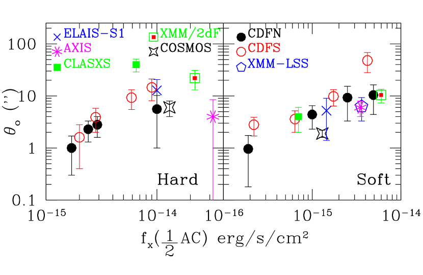
Figure 3: The angular correlation scale, $\theta_{0}$, as a function of different survey characteristic flux, defined as that corresponding to half the respective survey area-curves. Most results appear to be consistent with the clustering flux-limit dependence, found from the CDF-N and CDF-S. Note that in the left panel we plot the 4.5-10 keV results of Miyaji et al. (2007). Errorbars correspond to $1\sigma$ Poisson uncertainties.

In Figure 3 we plot the corresponding values of $\theta_{0}$ (for fixed $\gamma=1.8$) as a function of $f_{x}(\frac{1}{2}AC)$ (for both hard and soft bands) for the Chandra Large AREA Synoptic X-ray survey (CLASXS) (Yang et al. 2003), the XMM/2dF (Basilakos et al. 2004; 2005), XMM-COSMOS (Miyaji et al. 2007), XMM-ELAIS-S1 (Puccetti et al. 2006), XMM-LSS (Gandhi et al. 2006) and AXIS (Carrera et al. 2007) surveys. With the exception of the Yang et al. (2003) and the Carrera et al. (2007) hard-band results, the rest are consistent with the general flux-dependent trend. Note also that Gandhi et al. (2006) do not find any significant clustering of their hard-band sources. Of course, cosmic variance is also at work (as evidenced also by the clustering differences between the CDF-N and CDF-S; see Fig. 2 and Gilli et al. 2005) which should be responsible for the observed scatter around the main trend (see also Stewart et al. 2007).

We would like to stress that the CDF surveys have a large flux dynamical range which is necessary in order to investigate the $f_{x,{\rm limit}}-\theta_{o}$ correlation. This is probably why this effect has not been clearly detected in other surveys, although recently, a weak such effect was found also in the CLASXS survey (Yang et al. 2006).

3.3 The spatial correlation length using $w(\theta)$

We can use Limber’s equation to invert the angular clustering and derive the corresponding spatial clustering length, $r_{0}$ (eg. Peebles 1993). To do so it is necessary to model the spatial correlation function as a power law and to assume a clustering evolution model, which we take to be that of constant clustering in comoving coordinates (eg. de Zotti et al. 1990; Kundić 1997). For the inversion to be possible it is necessary to know the X-ray source redshift distribution, which can be determined by integrating the corresponding X-ray source luminosity function above the minimum luminosity that corresponds to the particular flux-limit used. To this end we use the Hasinger et al. (2005) and La Franca et al. (2005) LDDE luminosity functions for the soft and hard bands, respectively.

We perform the above inversion in the framework of the concordance $\Lambda$CDM cosmological model ($\Omega_{\rm m}=1-\Omega_{\Lambda}=0.3$) and the comoving clustering paradigm. The resulting values of the spatial clustering lengths, $r_{0}$, show the same dependence on flux-limits, as in Fig.2.

We can compare our results with direct determinations of the spatial-correlation function from Gilli et al. (2005), who used a smaller ($\sim 50\%$) spectroscopic sample from the CDF-N and CDF-S. They found a significant difference between the CDF-S and CDF-N clustering, with $r_{0}=10.3\pm 1.7\;h^{-1}$ Mpc and $r_{0}=5.5\pm 0.6\;h^{-1}$ Mpc, respectively (note also that the corresponding slopes were quite shallow, roughly $\gamma\simeq 1.4-1.5$). Since, Gilli et al. used sources from the full (0.5-8 keV) band, we compare their results with our soft-band results which, dominate the total-band sources. This comparison is possible, because as we have verified using a Kolmogorov-Smirnov test, the flux distributions of the sub-samples that have spectroscopic data are statistically equivalent with those of the whole samples. Our inverted clustering lengths, for the lowest flux-limit used, are: $r_{0}=10.3\pm 2\;h^{-1}$ Mpc and $r_{0}=6.4\pm 2.5\;h^{-1}$ Mpc (fixing $\gamma=1.8$) for the CDF-S and CDF-N respectively, in good agreement with the Gilli et al. (2005) direct 3D determination.

Our values can be also compared with the re-calculation of the CDF-N spatial clustering by Yang et al. (2006), who find $r_{0}\simeq 4.1\pm 1.1\;h^{-1}$ Mpc.

We return now to the strong trend between $\theta_{0}$ (or the corresponding $r_{0}$) and the sample flux-limit (see Fig.2 and 3), which could be due to two possible effects (or the combination of both). Either the different flux-limits correspond to different intrinsic luminosities, ie., a luminosity-clustering dependence (see also hints in the CLASXS and CDF-N based Yang et al. 2006 results; while for optical data see Porciani & Norberg 2006) or a redshift-dependent effect (ie., different flux-limits correspond to different redshifts traced). Using the sources which have spectroscopic redshift determinations we have derived their intrinsic luminosities, in each respective band, from their count rates using a spectral index $\Gamma=1.9$ and the concordance $\Lambda$CDM cosmology. We have also applied an absorption correction by assuming a power-law X-ray spectrum with an intrinsic $\Gamma=1.9$, obscured by an optimum column density to reproduce the observed hardness ratio. We then derive, for each flux-limit used, the median redshift and median luminosity of the corresponding sub-sample. We find relatively small variations and no monotonic change of the median redshift with subsample flux-limit. For example, the median spectroscopic redshift for the soft and hard bands, at the lowest flux-limit used, is ${\bar{z}}\sim 0.8$ and $\sim 0.95$, respectively, while its mean variation between the different flux-limits used is $\langle\delta z/z\rangle\simeq-0.11$ and -0.03 for the CDF-N and $\langle\delta z/z\rangle\simeq-0.27$ and 0.05 for the CDF-S soft and hard-bands, respectively. The large redshift variation of the soft-band CDF-S data should be attributed to the presence of a few superclusters at $z\sim 0.7$; see Gilli et al. 2003).

In Figure 4 we present the correlation between the subsample median X-ray luminosity and the corresponding subsample clustering length, as provided by Limber’s inversion. Although the CDF luminosity dynamical range is limited, it is evident that the median X-ray luminosity systematically increases with increasing sample flux-limit and it is correlated to $r_{0}$ (as expected from Fig.2). It should be noted that the correlation length of the highest-flux limited CDF-S soft-band subsample is by far the largest ever found ($\sim 30h^{-1}$ Mpc), but one has to keep in mind that the CDF-S appears not to be a typical field, as discussed earlier (see Gilli et al. 2003). The CDF-N high-flux results appear to converge to a value of $r_{0}\sim 18h^{-1}$ Mpc, similar to that of some other surveys (eg. Basilakos et al. 2004; 2005 and Puccetti et al. 2007).

We therefore conclude that not only are there indications for a luminosity dependent clustering of X-ray selected high-$z$ AGNs, but also that they are significantly more clustered than their lower-$z$ counterparts, which have $r_{0}\sim 7-8\;h^{-1}$ Mpc (eg. Akylas et al. 2000; Mullis et al. 2004). This is a clear indication of a strong bias evolution (eg. Basilakos, Plionis & Ragone-Figueroa 2007).

4 Conclusions

We have analysed the angular clustering of the CDF-N and CDF-S X-ray AGNs and find:

(1) A dependence of the angular clustering strength on the sample flux-limit. Most XMM and Chandra clustering analyses provide results that are consistent with the observed trend; a fact which appears to lift the confusion that arose from the apparent differences in their respective clustering lengths.

(2) Within the concordance cosmological model, the comoving clustering evolution model and the LDDE luminosity function, our angular clustering results are in good agreement with direct estimations of the CDF-N and CDF-S spatial clustering, which are based however on roughly half the total number of sources, for which spectroscopic data were available.

(3) The apparent correlation between clustering strength and sample flux-limit transforms into a correlation between clustering strength and intrinsic X-ray luminosity, since no significant redshift-dependent trend was found.

Table 1: The integrated angular clustering signal.

Sample	$f_{x,{\rm limit}}$a		$f_{x,{\rm limit}}$b
	$<400^{{}^{\prime\prime}}$	$<900^{{}^{\prime\prime}}$	$<400^{{}^{\prime\prime}}$	$<900^{{}^{\prime\prime}}$
CDF-N soft	$2.1\sigma$	$0.0\sigma$	$2.1\sigma$	$1.5\sigma$
CDF-N hard	$3.3\sigma$	$2.6\sigma$	$6.7\sigma$	$5.5\sigma$
CDF-S soft	$4.2\sigma$	$2.6\sigma$	$3.4\sigma$	$3.7\sigma$
CDF-S hard	$0.3\sigma$	$1.3\sigma$	$4.1\sigma$	$2.7\sigma$
a the lowest flux-limit.
b $5\times 10^{-16}$ erg s-1cm-2 (soft band) and $10^{-15}$ erg s-1cm-2 (hard band).

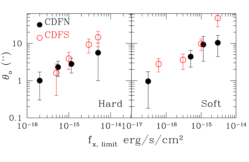
Figure 2: The angular clustering scale as a function of the flux-limit of the different samples. The dependence of clustering strength to the flux-limit is evident. The left and right panels correspond to the hard and soft bands respectively. Filled symbols correspond to the CDF-N while open ones to the CDF-S.

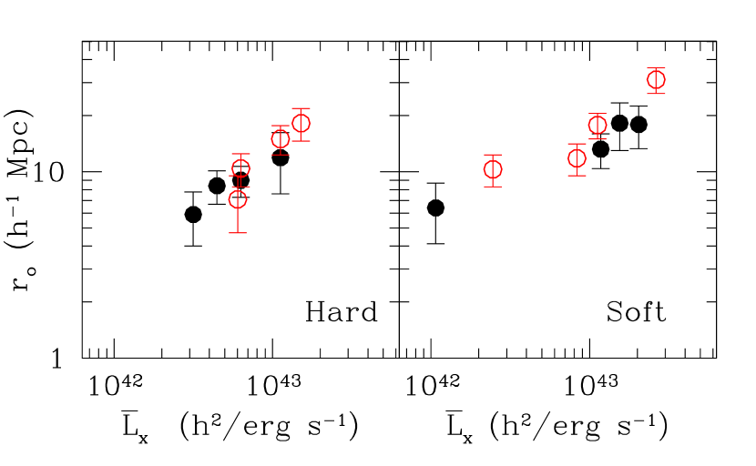
Figure 4: The correlation between the clustering length, $r_{0}$, and the median intrinsic X-ray luminosity of each subsample. The left and right panels correspond to the hard and soft bands respectively. Filled symbols correspond to the CDF-N while open ones to the CDF-S.

References

- (1) Akylas, A., Georgantopoulos, I., Plionis, M., 2000, MNRAS, 318, 1036
- (2) Alexander, D.M., et al., 2003, AJ, 126, 539
- (3) Basilakos, S. & Plionis, M., 2005, MNRAS, 360, L35
- (4) Basilakos, S. & Plionis, M., 2006, ApJ, 650, L1
- (5) Basilakos, S., Georgakakis, A., Plionis, M., Georgantopoulos, I., 2004, ApJL, 607, L79
- (6) Basilakos, S., Plionis, M., Georgantopoulos, I., Georgakakis, A., 2005, MNRAS, 356, 183
- (7) Basilakos, S., Plionis, M. & Ragone-Figueroa, 2007, ApJ, submitted
- (8) Barger, A.J., et al., 2003, AJ, 126, 632
- (9) Bauer, F.E., Alexander, D.M., Brandt, W.N., Schneider, D.P., Treister, E., Hornschemeier, A.E., Garmire, G.P., 2004, AJ, 128, 2048
- (10) Boyle B.J., Mo H.J., 1993, MNRAS, 260, 925
- (11) Carrera, F.J., Barcons, X., Fabian, A. C., Hasinger, G., Mason, K.O., McMahon, R.G., Mittaz, J.P.D., Page, M.J., 1998, MNRAS, 299, 229
- (12) Carrera, F.J., et al. 2007, A&A, 469, 27
- (13) de Zotti, G., Persic, M., Franceschini, A., Danese, L., Palumbo, G.G.C., Boldt, E.A., Marshall, F.E., 1990, ApJ, 351, 22
- (14) Gandhi, P., et al., 2006, A&A, 457, 393
- (15) Gilli, R., et al. 2003, ApJ, 592, 721
- (16) Gilli, R., et al. 2005, A&A, 430, 811
- (17) Giacconi, R., et al. 2001, ApJ, 551, 624
- (18) Hasinger, G., Miyaji, T., Schmidt, M., 2005, A&A, 441, 417
- (19) Kim, M., Wilkes, B.J., Kim, D-W., Green, P.J., Barkhouse, W.A., Lee, M.G., Silverman, J.D., Tananbaum, H.D., 2007, ApJ, 659, 29
- (20) Kundić, T., 1997, ApJ, 482, 631
- (21) La Franca, F. et al., 2005, ApJ, 635, 864
- (22) Le Févre, O., et al., 2004, A&A, 428, 1043
- (23) Lehmer, B.D., et al., 2005, ApJS, 161, 21
- (24) Manners, J.C., et al., 2003, MNRAS, 343, 293
- (25) Mignoli, M. et al., 1005, A&A, 437, 883
- (26) Miyaji, T., et al., 2007, ApJS, 172, 396
- (27) Mullis C.R., Henry, J. P., Gioia I. M., Böhringer H., Briel, U. G., Voges, W., Huchra, J. P., 2004, ApJ, 617, 192
- (28) Mo, H.J, & White, S.D.M 1996, MNRAS, 282, 347
- (29) Peebles P.J.E., 1993, “Principles of Physical Cosmology”, Princeton Univ. Press, Princeton, NJ
- (30) Peebles, P.J.E., 1973, ApJ, 185, 413
- (31) Plionis, M. & Basilakos, S., 2007, proceedings of the 6th International Workshop on the Identification of Dark Matter, held in Rhodes, Greece, astro-ph/0701696
- (32) Porciani, C. & Norberg, P., 2006, MNRAS, 371, 1824
- (33) Puccetti, S., et al., 2006, A&A, 457, 501
- (34) Sheth, R.K., Mo, H.J., Tormen, G., 2001, MNRAS, 323, 1
- (35) Stewart, G.C., 2007, in “X-ray Surveys: Evolution of Accretion, Star-Formation and the Large-Scale Structure”, Rodos island, Greece
- (36) http://www.astro.noa.gr/xray07/rodos-talks/
- (37) Szokoly, G.P., et al., 2004, ApJS, 155, 271
- (38) Vanzella, E., et al., 2005, A&A, 434, 53
- (39) Vanzella, E., et al., 2006, A&A, 454, 423
- (40) Vikhlinin, A. & Forman, W., 1995, ApJ, 455, 109
- (41) Yang, Y., Mushotzky, R.F., Barger, A.J., Cowie, L.L., Sanders, D.B., Steffen, A.T., 2003, ApJ, 585, L85
- (42) Yang, Y., Mushotzky, R.F., Barger, A.J., Cowie, L.L., 2006, ApJ, 645, 68