Estimates for the quenching time of a parabolic equation modeling electrostatic MEMS

Abstract

The singular parabolic problem $u_{t}=\Delta u-\frac{\lambda f(x)}{(1+u)^{2}}$ on a bounded domain $\Omega$ of ${\mathbb{R}}^{N}$ with Dirichlet boundary conditions, models the dynamic deflection of an elastic membrane in a simple electrostatic Micro-Electromechanical System (MEMS) device. In this paper, we analyze and estimate the quenching time of the elastic membrane in terms of the applied voltage —represented here by $\lambda$. As a byproduct, we prove that for sufficiently large $\lambda$, finite-time quenching must occur near the maximum point of the varying dielectric permittivity profile $f(x)$.

Key words: electrostatic MEMS; quenching time; quenching set.

1 Introduction

Micro-Electromechanical Systems (MEMS) are often used to combine electronics with micro-size mechanical devices in the design of various types of microscopic machinery. An overview of the physical phenomena of the mathematical models associated with the rapidly developing field of MEMS technology is given in [12]. The key component of many modern MEMS is the simple idealized electrostatic device shown in Figure 1. The upper part of this device consists of a thin and deformable elastic membrane that is held fixed along its boundary and which lies above a rigid grounded plate. This elastic membrane is modeled as a dielectric with a small but finite thickness. The upper surface of the membrane is coated with a negligibly thin metallic conducting film. When a voltage $V$ is applied to the conducting film, the thin dielectric membrane deflects towards the bottom plate, and when $V$ is increased beyond a certain critical value $V^{*}$ –known as pull-in voltage– the steady-state of the elastic membrane is lost, and proceeds to quenching, $i.e.$ snap through, at a finite time creating the so-called pull-in instability.

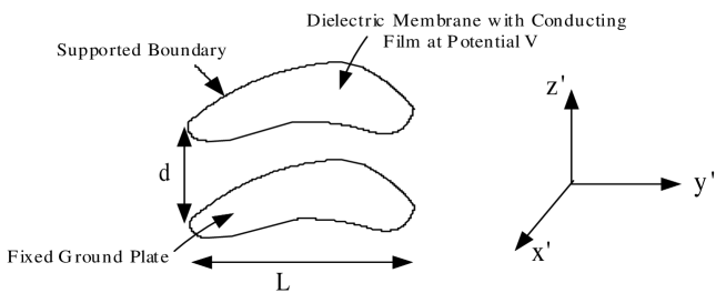
Figure 1: The simple electrostatic MEMS device.

A mathematical model of the physical phenomena, leading to a partial differential equation for the dimensionless dynamic deflection of the membrane, was derived and analyzed in [7]. In the damping-dominated limit, and using a narrow-gap asymptotic analysis, the dimensionless dynamic deflection $u=u(x,t)$ of the membrane on a bounded domain $\Omega$ in $\mathbb{R}^{2}$, is found to satisfy the following parabolic problem

$$\begin{array}[]{lll}u_{t}-\Delta u&=\displaystyle\frac{\lambda f(x)}{(1-u)^{2}}&{\rm for}\ x\in\Omega\,,\\[8.53581pt] \hfill u(x,t)&=0&{\rm for}\ x\in\partial\Omega\,,\\ \hfill u(x,0)&=0&{\rm for}\ x\in\Omega.\end{array}$$

The initial condition in $(P)_{\lambda}$ assumes that the membrane is initially undeflected and the voltage is suddenly applied to the upper surface of the membrane at time $t=0$. The parameter $\lambda>0$ in $(P)_{\lambda}$ characterizes the relative strength of the electrostatic and mechanical forces in the system, and is given in terms of the applied voltage $V$ by $\lambda=\frac{\varepsilon_{0}V^{2}L^{2}}{2T_{e}d^{3}}$, where $d$ is the undeflected gap size, $L$ is the length scale of the membrane, $T_{e}$ is the tension of the membrane, and $\varepsilon_{0}$ is the permittivity of free space in the gap between the membrane and the bottom plate. We shall use from now on the parameter $\lambda$ and $\lambda^{*}$ to represent the applied voltage $V$ and pull-in voltage $V^{*}$, respectively. Referred to as the permittivity profile, $f(x)$ in $(P)_{\lambda}$ is defined by the ratio $f(x)=\frac{\varepsilon_{0}}{\varepsilon_{2}(x)}$, where $\varepsilon_{2}(x)$ is the dielectric permittivity of the thin membrane.

Consider first the steady-state solutions of $(P)_{\lambda}$

$$\begin{array}[]{lll}\hfill-\Delta w&=&\displaystyle\frac{\lambda f(x)}{(1-w)^{2}}\,\ \ x\in\Omega,\\ \hfill w(x)&=&0\quad\quad\quad\quad x\in\partial\Omega\end{array}$$

with $0<w<1$ on $\Omega\subset\mathbb{R}^{N}$, and $f(x)$ was assumed to satisfy

$$\begin{array}[]{lll}\hbox{$f\in C^{\alpha}(\bar{\Omega})$ for some $\alpha\in(0,1]$, $0\leq f\leq 1$ and }\\ \hbox{$f>0$ on a subset of $\Omega$ with positive measure.}\end{array}$$ (1.1)

One can then easily show (e.g., Theorem 1.1 in [4]) that there exists a finite pull-in voltage $\lambda^{*}:=\lambda^{*}(\Omega,f)>0$ such that:

• $\bullet$  If $0\leq\lambda<\lambda^{*}$, there exists at least one solution for $(S)_{\lambda}$.

• $\bullet$  If $\lambda>\lambda^{*}$, there is no solution for $(S)_{\lambda}$.

Upper and lower bounds on the pull-in voltage $\lambda^{*}$ were also given in Theorem 1.1 of [4]. Fine properties of steady states –such as regularity, stability, uniqueness, multiplicity, energy estimates and comparison results– were shown in [3] and [4] to depend on the dimension of the ambient space and on the permittivity profile.

For the dynamic problem $(P)_{\lambda}$, we first define the following notion.

Definition 1.1.  (1)  A solution $u(x,t)$ of $(P)_{\lambda}$ is said to be quenching at a –possibly infinite– time $T=T(\lambda,f,\Omega)$, if the maximal value of $u$ reaches $1$ at time $T$.

(2)  A point $x_{0}\in\bar{\Omega}$ is said to be a quenching point for a solution $u(x,t)$ of $(P)_{\lambda}$, if for some $T\in(0,+\infty]$, we have $\lim\limits_{t_{n}\to T}u(x_{0},t_{n})=1$.

In [5] we dealt with issues of global convergence as well as quenching in finite or infinite time of the solutions of $(P)_{\lambda}$. One of the main results was the following relationship between the voltage $\lambda$ and the nature of the dynamic solution $u$ of $(P)_{\lambda}$.

Theorem A (Theorem 1.1 in [5]). Assuming that $f$ satisfies $(1.1)$ on a bounded domain $\Omega$, then the followings hold:

1. If $\lambda\leq\lambda^{*}$, then there exists a unique solution $u(x,t)$ for $(P)_{\lambda}$ which globally converges pointwise as $t\to+\infty$ to its unique minimal steady-state.

2. If $\lambda>\lambda^{*}$ and $\inf_{\Omega}f>0$, then the unique solution $u(x,t)$ of $(P)_{\lambda}$ must be quenching at a finite time.

A refined description of finite-time quenching behavior for $u$ was given in [6], where some quenching estimates, quenching rates, as well as some information on the properties of quenching set –such as compactness, location and shape, were obtained.

The first purpose of this paper is to prove –in Theorem 2.1– that quenching in finite-time occurs as soon as $\lambda>\lambda^{*}$, which means that Theorem A. 2. above holds without the restriction $\inf_{\Omega}f>0$. On the other hand, we continue our search for optimal estimates on quenching times at voltages $\lambda>\lambda^{*}$, since the latter translate into useful information on the operation speed of MEMS devices. Indeed, we established in Theorem 1.3 of [5], that if $\inf_{x\in\Omega}f(x)>0$, then the following upper estimate for the quenching time holds for any $\lambda>\lambda^{*}$:

$$T_{\lambda}(\Omega,f)\leq\frac{8(\lambda+\lambda^{*})^{2}}{3\inf_{x\in\Omega}f(x)(\lambda-\lambda^{*})^{2}(\lambda+3\lambda^{*})}\Big{[}1+\Big{(}\frac{\lambda+3\lambda^{*}}{2\lambda+2\lambda^{*}}\Big{)}^{1/2}\Big{]}.$$ (1.2)

In this paper, we shall improve this estimate –at least in dimensions less than 8– by proving that

$$T_{\lambda}(\Omega,f)\sim C\big{(}\lambda-\lambda^{*}\big{)}^{-\frac{1}{2}}\quad\quad\mbox{as}\quad\lambda\searrow\lambda^{*},$$

while

$$T\sim\frac{1}{3\lambda\sup_{x\in\bar{\Omega}}f(x)}\quad\mbox{as}\quad\lambda\nearrow\infty.$$

To be more precise, we first recall the following notions and results from [4]. For any solution $w$ of $(S)_{\lambda}$, we consider the linearized operator at $w$ defined by $L_{w,\lambda}=-\Delta-\frac{2\lambda f(x)}{(1-w)^{3}},$ and its corresponding eigenvalues $\{\mu_{k,\lambda}(w);k=1,2,...\}$. Say that a solution $w_{\lambda}$ of $(S)_{\lambda}$ is minimal, if $w_{\lambda}(x)\leq w(x)$ in $\Omega$ whenever $w$ is any solution of $(S)_{\lambda}$. We recall the following

Theorem B (Theorem 1.2 in [4]). Assume $f$ satisfies $(\ref{IV:permittivity})$ on a bounded domain $\Omega\subset\mathbb{R}^{N}$. Then,

• 1.  For any $0\leq\lambda<\lambda^{*}$, there exists a unique minimal solution $w_{\lambda}$ of $(S)_{\lambda}$ such that $\mu_{1,\lambda}(w_{\lambda})>0$. Moreover for each $x\in\Omega$, the function $\lambda\to w_{\lambda}(x)$ is strictly increasing and differentiable on $(0,\lambda^{*})$.

• 2.  If $1\leq N\leq 7$, then $w^{*}=\displaystyle\lim_{\lambda\uparrow\lambda^{*}}w_{\lambda}$ exists in $C^{1,\beta}(\bar{\Omega})$ which is then a solution for $(S)_{\lambda^{*}}$ such that $\mu_{1,\lambda^{*}}(w^{*})=0.$ In particular, $w^{*}$ –often referred to as the extremal solution of problem $(S)_{\lambda}$– is unique.

• 3.  On the other hand, if $N\geq 8$, $f(x)=|x|^{\alpha}$ with $0\leq\alpha\leq\alpha^{**}(N):=\frac{4-6N+3\sqrt{6}(N-2)}{4}$ and $\Omega$ is the unit ball, then the extremal solution is necessarily $w^{*}(x)=1-|x|^{\frac{2+\alpha}{3}}$ and is therefore singular.

We remark that in general, the function $w^{*}$ exists in any dimension, does solve $(S)_{\lambda^{*}}$ in a suitable weak sense and is the unique solution in an appropriate class. The above theorem says that it is however a classical solution in dimensions $1\leq N\leq 7$, that is

$$-\Delta w^{*}=\frac{\lambda^{*}f(x)}{(1-w^{*})^{2}}\quad\mbox{in}\ \Omega\,,\quad w^{*}>0\quad\mbox{in}\ \Omega\,,\quad w^{*}=0\quad\mbox{on}\ \partial\Omega\,,$$ (1.3)

and there exists an eigenfunction $\phi^{*}$ of $L_{{w^{*},\lambda^{*}}}$ satisfying

$$\Delta\phi^{*}+\frac{2\lambda^{*}\phi^{*}f(x)}{(1-w^{*})^{3}}=0\quad\mbox{in}\ \Omega\,,\quad\phi^{*}>0\quad\mbox{in}\ \Omega\,,\quad\phi^{*}=0\quad\mbox{on}\ \partial\Omega\,.$$ (1.4)

We denote by $\phi^{*}$ (resp., $\psi^{*}$) the corresponding unique $L^{2}$-normalized (resp., $L^{1}$-normalized) positive eigenfunction of $L_{{w^{*},\lambda^{*}}}$.

We shall then prove in section 2 the following upper and lower estimates on the quenching time $T=T(\lambda,f,\Omega)$ of a solution $u$ for $(P)_{\lambda}$ at voltage $\lambda>\lambda^{*}$: Under the condition that the unique extremal solution $w^{*}$ of $(S)_{\lambda}$ is regular, then

• For $\lambda$ sufficiently close to $\lambda^{*}$, we have the lower bound estimate

  $$T(\lambda,f,\Omega)\geq\Big{(}\frac{\sup_{x\in\Omega}\phi^{*}(x)}{12\lambda^{*}\sup_{x\in\Omega}\frac{f(x)}{(1-w^{*}(x))^{4}}\int_{\Omega}\frac{\phi^{*}}{(1-w^{*})^{2}}dx}\Big{)}^{\frac{1}{2}}\big{(}\lambda-\lambda^{*}\big{)}^{-\frac{1}{2}}.$$ (1.5)

• If $\int_{\Omega}\frac{\psi^{*}(x)}{f(x)}dx<\infty$, then for any $\lambda>\lambda^{*}$, we have the upper bound estimate

  $$T(\lambda,f,\Omega)\leq\frac{\sqrt{3}\pi}{4}\Big{(}\frac{\int_{\Omega}\frac{\psi^{*}(x)}{f(x)}dx}{\lambda^{*}\int_{\Omega}\psi^{*}(x)f(x)dx}\Big{)}^{\frac{1}{2}}\big{(}\lambda-\lambda^{*}\big{)}^{-\frac{1}{2}}\,.$$ (1.6)

Note that the above situation typically happens when $f\equiv|x|^{\beta}$ and $N\leq 7$, or for any $N>8$ provided $\beta$ is large. It would be interesting to establish similar estimates in the case where $w^{*}$ is singular. In the general case, we only have the following estimate established in section 3.

• There exist a constant $C=C(f,\Omega)>0$ and a sufficiently large $\lambda_{0}=\lambda_{0}(f,\Omega)>\lambda^{*}$ such that for any $\lambda>\lambda_{0}$, we have the estimates

  $$\frac{1}{3\lambda\sup_{x\in\bar{\Omega}}f(x)}\leq T(\lambda,f,\Omega)\leq\frac{1}{3\lambda\sup_{x\in\bar{\Omega}}f(x)}+\frac{C}{\lambda^{\frac{2+2\alpha}{2+\alpha}}}\,,$$ (1.7)

  where $\alpha\in(0,1]$ is as in $(\ref{IV:permittivity})$.

As a byproduct of the estimate (1.7), we shall analyze and compute in section 3 that in several situations, and at least for sufficiently large $\lambda$, quenching in finite-time must occur near the maximum point of the varying dielectric permittivity profile $f$. More precisely, if the quenching set $K$ of a solution $u$ for $(P)_{\lambda}$ is compact in $\Omega$, and if we are in one of the following two situations:

• 1)  $N=1$; or

• 2)  $N\geq 2$, $\Omega$ is a ball $B_{R}(0)$, $K=\{0\}$ and $f(r)$ is radially symmetric,

then for any $a\in K$, there exists $C>0$ such that for $\lambda$ large enough, we have

$$\big{(}\sup_{x\in\bar{\Omega}}f\big{)}^{\frac{1}{3}}-\big{(}f(a)\big{)}^{\frac{1}{3}}\leq\frac{C}{\lambda^{\frac{\alpha}{2+\alpha}}}\,,$$ (1.8)

We note that the compactness of the quenching set has been established in [6] (Proposition 2.1) in the case where the domain $\Omega$ is convex and $f$ satisfies both $(\ref{IV:permittivity})$ and the additional condition

$$\begin{array}[]{lll}\hbox{$\frac{\partial f}{\partial\nu}\leq 0\ $ on $\ \Omega^{c}_{\delta}:=\{x\in\Omega:\,dist(x,\partial\Omega)\leq\delta\}$ for some $\delta>0$.}\end{array}$$ (1.9)

Here $\nu$ is the outward unit norm vector to $\partial\Omega$. The above result can be seen as a refinement of Theorem 1.1 of [6] where it is proved that under the compactness assumption on the quenching set, the latter set cannot contain any zero of the profile $f$ (see also Lemma 3.2 below).

2 Quenching time for $\lambda>\lambda^{*}$

In this section, we establish the estimates on the quenching time of $(P)_{\lambda}$. First we borrow ideas from [1] to prove that we have quenching in finite time as soon as $\lambda>\lambda^{*}$, without the assumption used in [5] that $f$ is bounded away from zero.

Theorem 2.1.

If $\lambda>\lambda^{*}(\Omega,f)$, then the unique solution $u(x,t)$ of $(P)_{\lambda}$ must quench in finite time.

Proof. The uniqueness of solutions for $(P)_{\lambda}$ in $\Omega\times(0,\tau)$, where $\tau>0$ is the maximal existence time, was already noted in Proposition 2.1 of [5]. Let now $\lambda>\lambda^{*}$, and assume that $u=u(x,t)$ of $(P)_{\lambda}$ exists in $\Omega\times(0,\infty)$.

Given any $0<\varepsilon<\lambda-\lambda^{*}$, we first claim that $(P)_{\lambda-\varepsilon}$ has a global solution $u_{\varepsilon}$ that is uniformly bounded in $\Omega\times(0,\infty)$ by some constant $C_{\varepsilon}<1$. Indeed, set

$$g(u)=\frac{1}{(1-u)^{2}}\,,\quad h(u)=\int^{u}_{0}\frac{ds}{g(s)}\,,\quad 0\leq u\leq 1\,,$$ (2.1)

$$\widetilde{g}(u)=\frac{\lambda-\varepsilon}{\lambda(1-u)^{2}}\,,\quad\widetilde{h}(u)=\int^{u}_{0}\frac{ds}{\widetilde{g}(s)}\,,\quad 0\leq u\leq 1\,,$$ (2.2)

and let $\Phi_{\varepsilon}(u):=\widetilde{h}^{-1}\big{(}h(u)\big{)}$. Direct calculations show that

$$\Phi_{\varepsilon}(u)=1-\big{[}\frac{\varepsilon}{\lambda}+\frac{\lambda-\varepsilon}{\lambda}(1-u)^{3}\big{]}^{\frac{1}{3}}\leq C_{\varepsilon}<1\quad\mbox{for}\quad 0\leq u\leq 1\,,$$

where $C_{\varepsilon}=1-\big{(}\frac{\varepsilon}{\lambda}\big{)}^{\frac{1}{3}}$. Moreover, it is easy to check that $\Phi_{\varepsilon}(0)=0$, that $0\leq\Phi_{\varepsilon}(s)<s$ for $s\geq 0$, and that $\Phi_{\varepsilon}(s)$ is increasing and concave with

$$\Phi_{\varepsilon}^{\prime}(s)=\frac{\widetilde{g}(\Phi_{\varepsilon}(s))}{g(s)}>0\,.$$

Setting $v_{\varepsilon}=\Phi_{\varepsilon}(u)$, we have

$$\begin{array}[]{lll}&-\Delta v_{\varepsilon}=-\Phi_{\varepsilon}^{\prime\prime}(u)|\nabla u|^{2}-\Phi_{\varepsilon}^{\prime}(u)\Delta u&\\[5.69054pt] &\geq\Phi_{\varepsilon}^{\prime}(u)\big{(}\displaystyle\frac{\lambda f(x)}{(1-u)^{2}}-u_{t}\big{)}=\lambda f(x)\Phi_{\varepsilon}^{\prime}(u)g(u)-(v_{\varepsilon})_{t}&\\[5.69054pt] &=\lambda f(x)\widetilde{g}(\Phi_{\varepsilon}(u))-(v_{\varepsilon})_{t}=\displaystyle\frac{(\lambda-\varepsilon)f(x)}{(1-v_{\varepsilon})^{2}}-(v_{\varepsilon})_{t}\,,&\end{array}$$

and hence, $v_{\varepsilon}=\Phi_{\varepsilon}(u)\leq C_{\varepsilon}$ is therefore a supersolution of $(P)_{\lambda-\varepsilon}$. Since now zero is a subsolution of $(P)_{\lambda-\varepsilon}$, we deduce that there exists a unique global solution $u_{\varepsilon}$ for $(P)_{\lambda-\varepsilon}$ satisfying $0\leq u_{\varepsilon}\leq v_{\varepsilon}\leq C_{\varepsilon}<1$ uniformly in $\Omega\times(0,\infty)$, which gives our first claim.

Note that $(P)_{\lambda-\varepsilon}$ admits a Liapunov functional

$$V(u_{\varepsilon})=\frac{1}{2}\int_{\Omega}|\nabla u_{\varepsilon}|^{2}dx-(\lambda-\varepsilon)\int_{\Omega}\frac{f(x)}{1-u_{\varepsilon}}dx,\quad\dot{V}(u_{\varepsilon})=-\int_{\Omega}(u_{\varepsilon})^{2}_{t}dx.$$ (2.3)

Since now $\frac{1}{1-u_{\varepsilon}}$ is uniformly bounded in $\Omega\times(0,\infty)$, we obtain that for $\beta<1$,

$$\|u_{t}\|_{C^{0,\beta}},\ \|u_{tt}\|_{C^{0,\beta}}<C\quad\mbox{uniformly bounded in}\ \Omega\times(0,\infty)\,.$$ (2.4)

Moreover, (2.3) gives that $\int^{\infty}_{0}\int_{\Omega}(u_{\varepsilon})^{2}_{t}dx<\infty$, which means that $\int_{\Omega}(u_{\varepsilon})^{2}_{t}dx$ is a uniformly continuous function on $[0,\infty)$, and therefore

$$\int_{\Omega}(u_{\varepsilon})^{2}_{t}dx\to 0\quad\mbox{as}\quad t\to\infty\,.$$

Further, we deduce from (2.4) that $(u_{\varepsilon})_{t}\to 0$ as $t\to\infty$, which shows that there exists a function $0\leq w_{\varepsilon}(x)<C_{\varepsilon}<1$ on $\Omega$ such that $u_{\varepsilon}(x,t)\to w_{\varepsilon}(x)$ as $t\to\infty$, where $w_{\varepsilon}$ satisfies

$$-\Delta w_{\varepsilon}=\frac{(\lambda-\varepsilon)f(x)}{(1-w_{\varepsilon})^{2}}\quad\mbox{in}\ \Omega,\quad w_{\varepsilon}=0\quad\mbox{on}\ \partial\Omega\,.$$

Therefore, there exists a classical solution $w_{\varepsilon}$ of $(S)_{\lambda-\varepsilon}$ with $\lambda-\varepsilon>\lambda^{*}$, which contradicts the definition of $\lambda^{*}$, and completes the proof of Theorem 2.1. $\blacksquare$

2.1 Analytic estimates of quenching time

We now focus on estimating the quenching time $T$ when $\lambda>\lambda^{*}$, and in the case where the unique extremal solution $w^{*}$ of $(S)_{\lambda}$ is regular. This implies that $w^{*}$ satisfies

$$-\Delta w^{*}=\frac{\lambda^{*}f(x)}{(1-w^{*})^{2}}\quad\mbox{in}\ \Omega\,,\quad w^{*}>0\quad\mbox{in}\ \Omega\,,\quad w^{*}=0\quad\mbox{on}\ \partial\Omega\,,$$ (2.5)

and there exists an eigenfunction $\phi^{*}$ satisfying

$$\Delta\phi^{*}+\frac{2\lambda^{*}\phi^{*}f(x)}{(1-w^{*})^{3}}=0\quad\mbox{in}\ \Omega\,,\quad\phi^{*}>0\quad\mbox{in}\ \Omega\,,\quad\phi^{*}=0\quad\mbox{on}\ \partial\Omega\,.$$ (2.6)

We shall adapt and improve some of the arguments in [10]. Our first estimate is a lower bound for $T$ as stated in $(1.5)$.

Theorem 2.2.

Suppose that the unique extremal solution $w^{*}$ of $(S)_{\lambda}$ is regular. Then for $\lambda$ sufficiently close to $\lambda^{*}$, the finite quenching time $T(\lambda,f,\Omega)$ of the unique solution $u$ for $(P)_{\lambda}$ satisfies

$$T(\lambda,f,\Omega)\geq\Big{(}\frac{\sup_{x\in\Omega}\phi^{*}}{12\lambda^{*}\sup_{x\in\Omega}\frac{f(x)}{(1-w^{*})^{4}}\int_{\Omega}\frac{\phi^{*}}{(1-w^{*})^{2}}dx}\Big{)}^{\frac{1}{2}}\big{(}\lambda-\lambda^{*}\big{)}^{-\frac{1}{2}}\,,$$ (2.7)

where $\phi^{*}>0$ is the $L^{2}(\Omega)$-normalized eigenfunction satisfying (2.6).

Proof. Let $u^{*}$ be the unique solution of $(P)_{\lambda^{*}}$. First, we seek a bound on the rate at which $u^{*}$ approaches the corresponding steady-state $w^{*}$. For that, we set $u^{*}(x,t)=w^{*}(x)-\hat{u}(x,t)$. Then $\hat{u}(x,0)=w^{*}(x)$ in $\Omega$ and $\hat{u}=w^{*}$ on $\partial\Omega$. Moreover, we have

$$\begin{array}[]{lll}\displaystyle\frac{\partial\hat{u}}{\partial t}&=&\Delta\hat{u}-\Delta w^{*}-\displaystyle\frac{\lambda^{*}f(x)}{(1-w^{*}+\hat{u})^{2}}\\[8.53581pt] &=&\Delta\hat{u}+\lambda^{*}f(x)\Big{[}\displaystyle\frac{1}{(1-w^{*})^{2}}-\displaystyle\frac{1}{(1-w^{*}+\hat{u})^{2}}\Big{]}\\[11.38109pt] &\geq&\Delta\hat{u}+\displaystyle\frac{2\lambda^{*}\hat{u}f(x)}{(1-w^{*})^{3}}-\displaystyle\frac{3\lambda^{*}\hat{u}^{2}f(x)}{(1-w^{*})^{4}}\\[11.38109pt] &\geq&\Delta\hat{u}+\displaystyle\frac{2\lambda^{*}\hat{u}f(x)}{(1-w^{*})^{3}}-K_{1}\hat{u}^{2}\,,\end{array}$$ (2.8)

where $K_{1}=3\lambda^{*}\sup_{x\in\Omega}\frac{f(x)}{(1-w^{*})^{4}}$. Define

$$\psi=\frac{K_{2}\phi^{*}}{t+t_{0}}\,,\ \quad K_{2}=\frac{\sup_{x\in\Omega}\phi^{*}}{K_{1}},$$ (2.9)

where $t_{0}$ is chosen in such a way that

$$\psi(x,0)=\frac{K_{2}\phi^{*}}{t_{0}}\leq w^{*}(x)=\hat{u}(x,0)\quad\mbox{in}\quad\Omega.$$

Note that (2.9) gives

$$\Delta\psi+\displaystyle\frac{2\lambda^{*}\psi f(x)}{(1-w^{*})^{3}}-K_{1}\psi^{2}=-\frac{K_{1}K_{2}^{2}}{(t+t_{0})^{2}}(\phi^{*})^{2}\geq-\frac{K_{2}\phi^{*}}{(t+t_{0})^{2}}=\frac{\partial\psi}{\partial t},$$

and hence $0\leq\psi\leq\hat{u}=w^{*}-u^{*}$ in $\Omega\times(0,\infty)$.

We now set $u=u^{*}+u_{1}$, then $u_{1}$ satisfies

$$\begin{array}[]{lll}\displaystyle\frac{\partial u_{1}}{\partial t}&=&\Delta u_{1}+\displaystyle\frac{(\lambda-\lambda^{*})f(x)}{(1-u)^{2}}+\lambda^{*}f(x)\Big{[}\displaystyle\frac{1}{(1-u)^{2}}-\displaystyle\frac{1}{(1-u^{*})^{2}}\Big{]}\\[8.53581pt] &\leq&\Delta u_{1}+\displaystyle\frac{(\lambda-\lambda^{*})f(x)}{(1-w^{*})^{2}}+\displaystyle\frac{2\lambda^{*}u_{1}f(x)}{(1-w^{*})^{3}}\,,\end{array}$$ (2.10)

as long as $u=u^{*}+u_{1}\leq w^{*}$. We also define

$$I_{1}=\int_{\Omega}\frac{\phi^{*}}{(1-w^{*})^{2}}dx\,,\quad F(x)=\frac{f(x)}{\max\{1,\sup_{x\in\Omega}f(x)\}}\leq f(x),$$

and consider $\Phi^{*}(x)\geq 0$ to be a nonnegative solution of the problem

$$\begin{array}[]{lll}\hfill\Delta\Phi^{*}+\displaystyle\frac{2\lambda^{*}f(x)}{(1-w^{*})^{3}}\Phi^{*}+\displaystyle\frac{f(x)}{(1-w^{*})^{2}}-I_{1}\phi^{*}(x)F(x)&=&0\,\ \ x\in\Omega,\\ \hfill\Phi^{*}(x)&=&0\quad x\in\partial\Omega\,.\end{array}$$ (2.11)

Consider also the function

$$\psi_{1}=(\lambda-\lambda^{*})(I_{1}\phi^{*}t+\Phi^{*})\quad\mbox{in}\quad\Omega\times(0,\tau),$$ (2.12)

where $\tau>0$ is arbitrary. Then $\psi_{1}(x,0)=(\lambda-\lambda^{*})\Phi^{*}\geq 0=u_{1}(x,0)$ in $\Omega$, and $\psi_{1}(x,t)=0=u_{1}(x,0)$ on $\partial\Omega$. Moreover, since $F(x)\leq 1$ in $\Omega$, we obtain from $(\ref{L:7})$ and $(\ref{L:8})$ that

$$\begin{array}[]{lll}&(\psi_{1}-u_{1})_{t}-\Delta(\psi_{1}-u_{1})&\\[5.69054pt] =&(\lambda-\lambda^{*})I_{1}\phi^{*}-(\lambda-\lambda^{*})I_{1}t\Delta\phi^{*}-(\lambda-\lambda^{*})\Delta\Phi^{*}-(u_{1})_{t}+\Delta u_{1}&\\[5.69054pt] \geq&(\lambda-\lambda^{*})I_{1}\phi^{*}(x)-(\lambda-\lambda^{*})I_{1}\phi^{*}(x)F(x)+\displaystyle\frac{2\lambda^{*}f(x)}{(1-w^{*})^{3}}(\psi_{1}-u_{1})&\\[5.69054pt] \geq&\displaystyle\frac{2\lambda^{*}f(x)}{(1-w^{*})^{3}}(\psi_{1}-u_{1})&\end{array}$$

in $\Omega\times(0,\tau)$, as long as $u=u^{*}+u_{1}\leq w^{*}$. Therefore, the maximum principle implies that $\psi_{1}\geq u_{1}$ as long as $u=u^{*}+u_{1}\leq w^{*}$.

We now obtain that

$$u=u^{*}+u_{1}\leq w^{*}-\psi+\psi_{1}=w^{*}-\frac{K_{2}\phi^{*}}{t+t_{0}}+(\lambda-\lambda^{*})(I_{1}\phi^{*}t+\Phi^{*}).$$ (2.13)

But the right-hand side of $(\ref{L:11})$ is no larger than $w^{*}$, provided that

$$\frac{K_{2}\phi^{*}}{t+t_{0}}\geq(\lambda-\lambda^{*})(I_{1}\phi^{*}t+\Phi^{*})\quad\mbox{in}\quad\Omega\,,$$

which is equivalent to

$$K_{2}\geq(\lambda-\lambda^{*})(t+t_{0})(I_{1}t+A)\,,\quad\mbox{where}\quad A=\sup_{x\in\Omega}\frac{\Phi^{*}(x)}{\phi^{*}(x)}.$$

It requires

$$(\lambda-\lambda^{*})I_{1}t^{2}+(\lambda-\lambda^{*})(I_{1}t_{0}+A)t-K_{2}+A(\lambda-\lambda^{*})t_{0}\leq 0,$$

which is

$$t\leq\displaystyle\frac{-(\lambda-\lambda^{*})(I_{1}t_{0}+A)+\sqrt{\Delta}}{2I_{1}(\lambda-\lambda^{*})},$$ (2.14)

where

$$\Delta:=(\lambda-\lambda^{*})^{2}(I_{1}t_{0}+A)^{2}+4I_{1}(\lambda-\lambda^{*})\big{(}K_{2}-At_{0}(\lambda-\lambda^{*})\big{)}.$$

For $\lambda$ sufficiently close to $\lambda^{*}$, $(\ref{L:12})$ can be satisfied if

$$t\leq\frac{1}{2}\sqrt{\frac{K_{2}}{I_{1}}}(\lambda-\lambda^{*})^{-\frac{1}{2}}:=T_{L}.$$

Note that $T_{L}$ is given by

$$T_{L}=\Big{(}\frac{\sup_{x\in\Omega}\phi^{*}(x)}{12\lambda^{{}^{*}}\sup_{x\in\Omega}\frac{f(x)}{(1-w^{*})^{4}}\int_{\Omega}\frac{\phi^{*}}{(1-w^{*})^{2}}dx}\Big{)}^{\frac{1}{2}}\big{(}\lambda-\lambda^{*}\big{)}^{-\frac{1}{2}}.$$

Therefore, we conclude from (2.13) that $u\leq w^{*}$ in $\Omega\times(0,T_{L}]$. This implies that the finite quenching time $T$ of $u$ satisfies $T\geq T_{L}$, and the proof is complete. $\blacksquare$

We now establish the upper bound on $T$ as stated in $(1.6)$.

Theorem 2.3.

Suppose that the unique extremal solution $w^{*}$ of $(S)_{\lambda}$ is regular, and that $\int_{\Omega}\frac{\psi^{*}(x)}{f(x)}dx<\infty$, where $\psi^{*}>0$ is the $L^{1}(\Omega)$-normalized eigenfunction satisfying (2.6). Then for any $\lambda>\lambda^{*}$, the finite quenching time $T=T(\lambda,f,\Omega)$ of the unique solution $u$ for $(P)_{\lambda}$ satisfies

$$T(\lambda,f,\Omega)\leq\frac{\sqrt{3}\pi}{4}\Big{(}\frac{\int_{\Omega}\frac{\psi^{*}(x)}{f(x)}dx}{\lambda^{*}\int_{\Omega}\psi^{*}(x)f(x)dx}\Big{)}^{\frac{1}{2}}\big{(}\lambda-\lambda^{*}\big{)}^{-\frac{1}{2}}\,.$$ (2.15)

Proof. Setting $u=w^{*}+v$, then we have

$$\begin{array}[]{lll}\displaystyle\frac{\partial v}{\partial t}&=&\Delta w^{*}+\Delta v+\displaystyle\frac{(\lambda-\lambda^{*})f(x)}{(1-u)^{2}}+\displaystyle\frac{\lambda^{*}f(x)}{[1-(w^{*}+v)]^{2}}\\[11.38109pt] &=&\Delta v+\displaystyle\frac{2\lambda^{*}vf(x)}{(1-w^{*})^{3}}+\displaystyle\frac{(\lambda-\lambda^{*})f(x)}{(1-u)^{2}}\\[8.53581pt] &&+\lambda^{*}f(x)\displaystyle\Big{[}\frac{1}{[1-(w^{*}+v)]^{2}}-\frac{1}{(1-w^{*})^{2}}-\frac{2v}{(1-w^{*})^{3}}\Big{]}\,.\end{array}$$ (2.16)

Multiplying $(\ref{time:2.6})$ by $\psi^{*}$ and integrating over $\Omega$, we obtain

$$\displaystyle\frac{d}{dt}\int_{\Omega}\psi^{*}vdx = (\lambda-\lambda^{*})\displaystyle\int_{\Omega}\frac{\psi^{*}f(x)}{(1-u)^{2}}dx$$

$$+\lambda^{*}\displaystyle\int_{\Omega}\psi^{*}f(x)\Big{[}\frac{1}{[1-(w^{*}+v)]^{2}}-\displaystyle\frac{1}{(1-w^{*})^{2}}-\displaystyle\frac{2v}{(1-w^{*})^{3}}\Big{]}dx,$$

where (2.6) is applied. We next define

$$E(t)=\int_{\Omega}\psi^{*}vdx\,,\quad E(0)=-\int_{\Omega}\psi^{*}w^{*}dx=-E_{0}\in(-1,0);$$

$$I_{1}=\int_{\Omega}\psi^{*}(x)f(x)dx\leq\int_{\Omega}\frac{\psi^{*}(x)f(x)}{(1-u)^{2}}dx\,,\quad I_{2}=\displaystyle\frac{3\lambda^{*}}{\int_{\Omega}\frac{\psi^{*}(x)}{f(x)}dx}.$$

Using the inequalities

$$\begin{array}[]{lll}\displaystyle\frac{1}{[1-(w^{*}+v)]^{2}}-\displaystyle\frac{1}{(1-w^{*})^{2}}-\displaystyle\frac{2v}{(1-w^{*})^{3}}&\geq&\left\{\begin{array}[]{lll}\frac{3v^{2}}{(1-w^{*})^{4}},\quad\mbox{if}\quad v\geq 0;\\[2.84526pt] \frac{3v^{2}}{(1-u)^{4}},\ \,\quad\mbox{if}\quad v\leq 0;\\ \end{array}\right.\end{array}$$

the Hölder inequality yields that

$$\begin{array}[]{lll}&\lambda^{*}\displaystyle\int_{\Omega}\psi^{*}f(x)\Big{[}\frac{1}{[1-(w^{*}+v)]^{2}}-\frac{1}{(1-w^{*})^{2}}-\frac{2v}{(1-w^{*})^{3}}\Big{]}dx&\\[11.38109pt] &\geq 3\lambda^{*}\displaystyle\int_{\Omega}v^{2}\psi^{*}(x)f(x)dx\geq\displaystyle\frac{3\lambda^{*}}{\int_{\Omega}\frac{\psi^{*}(x)}{f(x)}dx}\Big{(}\int_{\Omega}\psi^{*}vdx\Big{)}^{2}=I_{2}E^{2}(t)\,.&\end{array}$$

It follows from the above that

$$\frac{dE}{dt}\geq(\lambda-\lambda^{*})I_{1}+I_{2}E^{2}\,,\quad E(0)=-E_{0}\in(-1,0).$$ (2.17)

We now compare $E(t)$ with the solution $F(t)$ of

$$\frac{dF}{dt}=(\lambda-\lambda^{*})I_{1}+I_{2}F^{2}\,,\quad F(0)=-E_{0}\in(-1,0).$$ (2.18)

Standard comparison principle yields that $E(t)\geq F(t)$ on their domains of existence. Therefore,

$$\sup_{\Omega}v\geq E(t)\geq F(t)\,.$$ (2.19)

It is easy to see from (2.18) that the quenching time $\bar{T}_{1}$ for $F(t)$ is given by

$$\begin{array}[]{lll}\bar{T}_{1}&\equiv&\Big{(}\displaystyle\frac{\pi}{4}+\arctan\sqrt{\frac{I_{2}}{(\lambda-\lambda^{*})I_{1}}}\Big{)}\Big{(}(\lambda-\lambda^{*})I_{1}I_{2}\Big{)}^{-\frac{1}{2}}\\[11.38109pt] &\leq&\displaystyle\frac{\sqrt{3}\pi}{4}\Big{(}\displaystyle\frac{\int_{\Omega}\frac{\psi^{*}(x)}{f(x)}dx}{\lambda^{*}\int_{\Omega}\psi^{*}(x)f(x)dx}\Big{)}^{\frac{1}{2}}\big{(}\lambda-\lambda^{*}\big{)}^{-\frac{1}{2}}\,.\end{array}$$

Therefore, for any $\lambda>\lambda^{*}$ the unique solution $u$ of $(P)_{\lambda}$ must quench at a finite time $T=T(\lambda,f,\Omega)\leq\bar{T}_{1}$, and we are done. $\blacksquare$

3 Quenching behavior for sufficiently large $\lambda$

In this section we discuss the quenching behavior of solutions of $(P)_{\lambda}$ for $\lambda$ large enough. We begin with the following refined estimates for the quenching time as stated in $(1.7)$.

Lemma 3.1.

Assume $f$ satisfies $(\ref{IV:permittivity})$ on a bounded domain $\Omega$, and suppose $u$ is a quenching solution of $(P)_{\lambda}$ at finite time $T$. Then, there exist a constant $C=C(f,\Omega)>0$ and a sufficiently large $\lambda_{0}=\lambda_{0}(f,\Omega)>0$ such that for any $\lambda>\lambda_{0}$, we have

$$\frac{1}{3\lambda\sup_{x\in\bar{\Omega}}f(x)}\leq T\leq\frac{1}{3\lambda\sup_{x\in\bar{\Omega}}f}+\frac{C}{\lambda^{\frac{2+2\alpha}{2+\alpha}}}\,,$$ (3.1)

where $\alpha\in(0,1]$ is as in $(\ref{IV:permittivity})$.

Proof. In order to obtain the lower bound of finite time $T$, we consider the initial value problem:

$$\begin{array}[]{lll}\displaystyle\frac{d\eta(t)}{dt}&=&\displaystyle\frac{\lambda M}{(1-\eta(t))^{2}}\,,\\[5.69054pt] \hfill\eta(0)&=&0\,,\end{array}$$ (3.2)

where $M=\sup_{x\in\bar{\Omega}}f(x)$. From $(\ref{3:14})$ one has $\frac{1}{\lambda M}\int_{0}^{\eta(t)}(1-s)^{2}ds=t\,.$ If $T_{*}$ is the time where $\lim_{t\to T_{*}}\eta(t)=1$, then we have $T_{*}=\frac{1}{\lambda M}\int_{0}^{1}(1-s)^{2}ds=\frac{1}{3\lambda M}.$ Obviously, $\eta(t)$ is now a super-solution of $u(x,t)$ near quenching, and thus we have

$$T\geq T_{*}=\frac{1}{3\lambda M}=\frac{1}{3\lambda\sup_{x\in\bar{\Omega}}f(x)}\,,$$

which is true for any $\lambda>0$.

We next prove the upper bound in (3.1). Let $\bar{a}\in\bar{\Omega}$ be such that $f(\bar{a})=\sup_{x\in\bar{\Omega}}f(x)$, and suppose $K=K(f,\Omega)$ is the Hölder constant of $f$. Since $f\in C^{\alpha}(\bar{\Omega})$ for some $\alpha\in(0,1]$, then for any sufficiently small $\varepsilon>0$, there exists $\delta=\big{(}\frac{\varepsilon}{2K}\big{)}^{1/\alpha}$ such that

$$f(x)\geq f(\bar{a})-\frac{\varepsilon}{2}\,,\quad\forall x\in Q:=B(\bar{a},\delta)\cap\Omega\,,$$

where $B(\bar{a},\delta)$ is a ball centered at $\bar{a}$ with radius $\delta$. Let $v$ be the solution of

$$\begin{array}[]{lll}\hfill v_{t}-\Delta v&=&\displaystyle\frac{\lambda\big{(}f(\bar{a})-\frac{\varepsilon}{2}\big{)}}{(1-v)^{2}}\quad\mbox{in}\ Q\times(0,T_{v})\,,\\[5.69054pt] \hfill v(x,0)=0\quad\mbox{in}&Q\,,&\quad v(x,t)=0\quad\mbox{on}\ \partial Q\times(0,T_{v})\,,\end{array}$$ (3.3)

where $T_{v}$ is the maximal existence time of $(\ref{IV:time:3})$. Comparison arguments shows that $u\geq v$ in $Q\times(0,T_{m})$, where $T_{m}=\min\{T,T_{v}\}$. Therefore, we have $T\leq T_{v}$.

Our goal now is to estimate $T_{v}$ for sufficiently large values of $\lambda$. Let $\mu_{1}(\delta)$ be the first eigenvalue of $-\Delta$ in $B(\bar{a},\delta)$, and let $\phi$ be the corresponding positive eigenfunction normalized such that $\int_{Q}\phi dx=1$. Multiplying $(\ref{IV:time:3})$ by $\phi$ and integrating over $Q$, we obtain

$$\begin{array}[]{lll}\displaystyle\frac{d}{dt}\int_{Q}\phi v\,dx&=&\displaystyle\int_{Q}\phi\Delta v\,dx+\displaystyle\lambda\big{(}f(\bar{a})-\frac{\varepsilon}{2}\big{)}\int_{Q}\frac{\phi}{(1-v)^{2}}\,dx\\[8.53581pt] &=&-\mu_{1}(\delta)\displaystyle\int_{Q}\phi v\,dx+\displaystyle\lambda\big{(}f(\bar{a})-\frac{\varepsilon}{2}\big{)}\int_{Q}\frac{\phi}{(1-v)^{2}}\,dx\,.\end{array}$$ (3.4)

Next, we define an energy-like quantity by $E(t)=\int_{Q}\phi_{{}_{\Omega}}v\,dx$ so that $E(0)=0$ and

$$E(t)=\int_{Q}\phi_{{}_{\Omega}}v\,dx\leq\sup_{Q}{v}\int_{Q}\phi\,dx=\sup_{Q}v\,.$$ (3.5)

Then, using Jensen’s inequality on the right-hand side of (3.4), we obtain

$$\frac{dE}{dt}+\mu_{1}(\delta)E\geq\frac{\lambda\big{(}f(\bar{a})-\frac{\varepsilon}{2}\big{)}}{(1-E)^{2}}\,,\qquad E(0)=0\,.$$

Recall that there exists a constant $D=D(N)>0$, depending only on $N$, such that $\mu_{1}(\delta)=D\delta^{-2}$. We now choose $\varepsilon=\varepsilon(\lambda,f,\Omega)>0$ such that

$$\mu_{1}(\delta)=D\delta^{-2}=D\big{(}\frac{\varepsilon}{2K}\big{)}^{-\frac{2}{\alpha}}=\frac{\lambda}{2}\varepsilon\,,\quad i.e.,\quad\varepsilon=\frac{2D^{\frac{\alpha}{2+\alpha}}K^{\frac{2}{2+\alpha}}}{\lambda^{\frac{\alpha}{2+\alpha}}}.$$ (3.6)

Then there exists a sufficiently large $\lambda_{0}=\lambda_{0}(f,\Omega)>\lambda^{*}$ such that for any $\lambda>\lambda_{0}$, we have $f(\bar{a})-\varepsilon>0$ and

$$\begin{array}[]{lll}\displaystyle\frac{dE}{dt}&\geq&\displaystyle\frac{\lambda\big{(}f(\bar{a})-\varepsilon\big{)}}{(1-E)^{2}}+\displaystyle\frac{\lambda\varepsilon}{2(1-E)^{2}}-\mu_{1}(\delta)E\\[5.69054pt] &\geq&\displaystyle\frac{\lambda\big{(}f(\bar{a})-\varepsilon\big{)}}{(1-E)^{2}}+\displaystyle\frac{\lambda\varepsilon}{2}-\mu_{1}(\delta)=\displaystyle\frac{\lambda\big{(}f(\bar{a})-\varepsilon\big{)}}{(1-E)^{2}}\,.\end{array}$$

This implies a finite quenching time $T_{E}$ of $E$ satisfying

$$T_{E}\leq\frac{1}{3\lambda\big{(}f(\bar{a})-\varepsilon\big{)}}\leq\frac{1}{3\lambda f(\bar{a})}+\frac{C}{\lambda^{\frac{2+2\alpha}{2+\alpha}}}\,,$$

where $C=C(f,\Omega)$ is independent of $\lambda$ in view of (3.6). Therefore, we conclude from $(\ref{IV:time:7})$ that

$$T\leq T_{v}\leq T_{E}\leq\frac{1}{3\lambda f(\bar{a})}+\frac{C}{\lambda^{\frac{2+2\alpha}{2+\alpha}}}\,,$$

and the lemma is proved. $\blacksquare$

We now recall the following result proved in Theorem 1.1 of [6].

Lemma 3.2.

Assume $f$ satisfies $(\ref{IV:permittivity})$ for some $\alpha\in(0,1]$ on a bounded domain $\Omega\subset\mathbb{R}^{N}$, and let $u$ be a quenching solution of $(P)_{\lambda}$ at finite time $T$. Assuming the quenching set of $u$ is compact in $\Omega$, then

1. No point $a\in\bar{\Omega}$ satisfying $f(a)=0$ can be a quenching point of $u$;

2. There exists a constant $M>0$ such that

   $$M(T-t)^{\frac{1}{3}}\leq 1-u(x,t)\quad\mbox{in}\quad\Omega\times(0,T).$$ (3.7)

The following result can now be seen as a converse of Lemma 3.2: for sufficiently large $\lambda$, finite-time quenching must occur near the maximum point of the varying dielectric permittivity profile $f$.

Theorem 3.3.

Assume $f$ satisfies $(\ref{IV:permittivity})$ for some $\alpha\in(0,1]$ on a bounded domain $\Omega\subset\mathbb{R}^{N}$, and suppose that $u$ is a quenching solution of $(P)_{\lambda}$ at finite time $T$, in such a way that the quenching set $K$ of $u$ is compact in $\Omega$. Then, for any $a\in K$, there exists $C>0$ such that for $\lambda$ large enough, we have

$$\big{(}\sup_{x\in\bar{\Omega}}f\big{)}^{\frac{1}{3}}-\big{(}f(a)\big{)}^{\frac{1}{3}}\leq\frac{C}{\lambda^{\frac{\alpha}{2+\alpha}}}\,,$$ (3.8)

provided we are in one the following two situations:

• 1)  $N=1$; or

• 2)  $N\geq 2$ and $a=0$, $\Omega$ is a ball $B_{R}(0)$ and $f(r)$ is radially symmetric.

Proof. The idea of the proof –inspired by [2]– is to combine the estimates on quenching time given by Lemma 3.1, with the local energy estimates near any quenching point established in [6]. Given a quenching point $a$ of $u$ and its corresponding quenching time $T$, we define

$$y=\frac{x-a}{\sqrt{T-t}}\,,\quad s=-\log(1-\frac{t}{T})\,,\quad 1-u(x,t)=(T-t)^{\frac{1}{3}}w(y,s),$$

then $w$ satisfies

$$\rho w_{s}=\nabla\cdot(\rho\nabla w)+\frac{1}{3}\rho w-\frac{\lambda\rho f(a+yT^{\frac{1}{2}}e^{-\frac{s}{2}})}{w^{2}}\quad\mbox{in}\quad\Omega(s)\times(0,\infty)\,,$$

where $\rho(y)=e^{-|y|^{2}/4}$ and $\Omega(s)=\{y:a+yT^{\frac{1}{2}}e^{-\frac{s}{2}}\in\Omega\}$. The compactness assumption on the quenching set implies that there exists a sufficiently large $s_{0}>0$ such that $B_{s}(a)\subset\Omega(s)$ for any $s\geq s_{0}$.

Consider now the “frozen” energy functional

$$E(w)=\frac{1}{2}\int_{B_{s}}\rho|\nabla w|^{2}dy-\frac{1}{6}\int_{B_{s}}\rho w^{2}dy-\int_{B_{s}}\frac{\lambda\rho f(a)}{w}dy\,,$$

which is defined in the compact set $B_{s}$ of $\Omega_{a}(s)$ for $s\geq s_{0}$. Note from Lemma 3.2 that $f(a)>0$. Using the same argument of Lemma 2.10 in [6], one can obtain

$$\begin{array}[]{lll}\displaystyle\int_{B_{s}}\rho|w_{s}|^{2}dy&\leq&-\displaystyle\frac{dE}{ds}+\displaystyle\int_{\partial B_{s}}\rho w_{s}\frac{\partial w}{\partial\nu}dS+\displaystyle\frac{1}{2s}\int_{\partial B_{s}}\rho|\nabla w|^{2}(y\cdot\nu)dS\\[11.38109pt] &&+\displaystyle\int_{B_{s}}\frac{\lambda\rho w_{s}[f(a)-f(a+yT^{\frac{1}{2}}e^{-\frac{s}{2}})]}{w^{2}}dy\\[11.38109pt] &:=&-\displaystyle\frac{dE}{ds}+I_{1}+I_{2}+I_{3}\,,\end{array}$$ (3.9)

where

$$I_{1}\leq C_{1}s^{N}e^{-\frac{s^{2}}{4}+\frac{s}{3}}\,,\quad I_{2}\leq C_{3}s^{N-1}e^{-\frac{s^{2}}{4}}.$$

To estimate $I_{3}$, we use Lemma 3.2 to infer that $w$ has a lower bound, and since $f\in C^{\alpha}(\bar{\Omega})$, we apply Hölder’s inequality to deduce that

$$I_{3}\leq CT^{\frac{\alpha}{2}}e^{-\frac{\alpha}{2}s}\int_{B_{s}}\rho|y|^{\alpha}w_{s}dy\leq CT^{\frac{\alpha}{2}}e^{-\frac{\alpha}{2}s}\Big{(}\int_{B_{s}}\rho|w_{s}|^{2}dy\Big{)}^{\frac{1}{2}}.$$

Therefore, (3.9) gives for $s\gg 1$,

$$\frac{dE}{ds}\leq-\displaystyle\int_{B_{s}}\rho|w_{s}|^{2}dy+CT^{\frac{\alpha}{2}}e^{-\frac{\alpha}{2}s}\Big{(}\int_{B_{s}}\rho|w_{s}|^{2}dy\Big{)}^{\frac{1}{2}}+Cs^{N}e^{-\frac{s^{2}}{4}+\frac{s}{3}}.$$ (3.10)

Maximizing now the right hand side of (3.10) with respect to $\displaystyle\int_{B_{s}}\rho|w_{s}|^{2}dy$, it yields that for $s\gg 1$

$$\frac{dE}{ds}\leq CT^{\alpha}e^{-\alpha s}+Cs^{N}e^{-\frac{s^{2}}{4}+\frac{s}{3}}\leq CT^{\alpha}e^{-\alpha s}.$$

This leads to

$$E(w)\leq E\big{(}w(y,0)\big{)}+\frac{CT^{\alpha}}{\alpha}=E(T^{-\frac{1}{3}})+\frac{CT^{\alpha}}{\alpha}\,.$$

Under the compactness assumption on the quenching set, a proof similar to Theorem 1.3 in [6] (see also [8, 9]) gives that

$$\lim_{s\to\infty}w(y,s)=\big{(}3\lambda f(a)\big{)}^{\frac{1}{3}}:=k(a)$$

uniformly on $|y|\leq C$ for any bounded constant $C$, and $E(w(\cdot,s))\to E(k(a))$ as $s\to\infty$, provided one of the following conditions holds:

• 1)  $N=1$; or

• 2)  $N\geq 2$ and $a=0$, $\Omega=B_{R}(0)$ is a bounded ball and $f(r)=f(|x|)$ is radially symmetric.

Therefore, under the assumption of Theorem 3.3, we have the following upper bound

$$E(k(a))\leq E(T^{-\frac{1}{3}})+\frac{CT^{\alpha}}{\alpha}\,.$$ (3.11)

Observe that if $b$ is a constant then the energy $E$ can be rewritten as $E(b)=\Gamma F(b)$, where $\Gamma=\int\rho(y)dy$ and $F$ is the function

$$F(z)=-\frac{1}{6}z^{2}-\frac{\lambda f(a)}{z}\,,\quad z>0\,.$$

Since $F$ attains a unique maximum at $k(a)$ and $F^{\prime\prime}(k(a))=-1$, there exist $\gamma$ and $\beta$ such that if $|z-k(a)|\leq\gamma$ then $F^{\prime\prime}(z)\leq-\frac{1}{2}$, and if $|F(z)-F(k(a))|\leq\beta$ then $|z-k(a)|\leq\gamma$. So we obtain from $(\ref{IV:time:9})$ that

$$F(k(a))\leq F(T^{-\frac{1}{3}})+\frac{CT^{\alpha}}{\alpha}\,.$$

Choose $\lambda_{1}$ such that $\frac{CT^{\alpha}}{\alpha}=\beta$. Then for $\lambda>\max\{\lambda_{0},\lambda_{1}\}$, where $\lambda_{0}$ is as in Lemma 3.1, we have

$$\beta\geq\frac{CT^{\alpha}}{\alpha}\geq F(k(a))-F(T^{-\frac{1}{3}})\,.$$

Hence from the properties of $F$, we have $k(a)-T^{-\frac{1}{3}}\leq\gamma$, which implies $F^{\prime\prime}(k(a))\leq-\frac{1}{2}$. It now deduces from (3.11) that

$$\frac{C}{\alpha\lambda^{\alpha}}\geq\frac{CT^{\alpha}}{\alpha}\geq F(k(a))-F(T^{-\frac{1}{3}})\geq\frac{1}{4}[T^{-\frac{1}{3}}-k(a)]^{2},$$

where Lemma 3.1 is applied in the first inequality. This further gives that

$$T^{-\frac{1}{3}}-\big{(}3\lambda f(a)\big{)}^{\frac{1}{3}}\leq\frac{C}{\lambda^{\frac{\alpha}{2}}}\,.$$ (3.12)

On the other hand, since Lemma 3.1 gives

$$T\leq\frac{1}{3\lambda\sup_{x\in\bar{\Omega}}f}+\frac{C}{\lambda^{\frac{2+2\alpha}{2+\alpha}}}\leq\frac{1}{3\lambda\sup_{x\in\bar{\Omega}}f}\Big{(}1+\frac{C}{\lambda^{\frac{\alpha}{2+\alpha}}}\Big{)}\,,$$

we have

$$T^{-\frac{1}{3}}\geq\big{(}3\lambda\sup_{x\in\bar{\Omega}}f(x)\big{)}^{\frac{1}{3}}\Big{(}1-\frac{C}{\lambda^{\frac{\alpha}{2+\alpha}}}\Big{)}\,.$$

Therefore, we finally conclude that

$$\big{(}\sup_{x\in\bar{\Omega}}f(x)\big{)}^{\frac{1}{3}}-\big{(}f(a)\big{)}^{\frac{1}{3}}\leq\frac{C}{\lambda^{\frac{1}{3}+\frac{\alpha}{2}}}+\frac{C}{\lambda^{\frac{\alpha}{2+\alpha}}}\leq\frac{C}{\lambda^{\frac{\alpha}{2+\alpha}}}.$$

This completes the proof of Theorem 3.3. $\blacksquare$

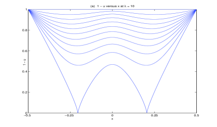
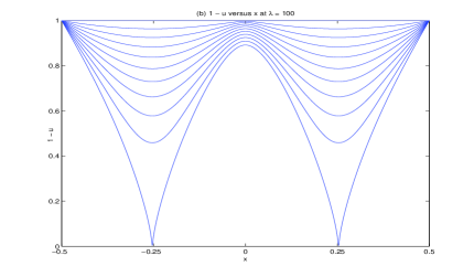
Figure 2: Left figure $(a)$: plots of $1-u$ versus $x$ at different times, where $\lambda=10$. Right figure $(b)$: plots of $1-u$ versus $x$ at different times, where $\lambda=100$.

Before ending this section, we now present a few numerical simulations on Lemma 3.1 and Theorem 3.3. Here we apply the implicit Crank-Nicholson scheme (see §3.2 of [7] for details), with the meshpoints $N=6000$, to $(P)_{\lambda}$ in the symmetric slab domain $-1/2\leq x\leq 1/2$. We choose the varying dielectric permittivity profile $f(x)$ satisfying

$$f[\alpha](x)=\left\{\begin{array}[]{ll}1-16(x+1/4)^{2}\,,&\mbox{if}\ \ \ x<-1/4\,;\\ |\sin(2\pi x)|\,,&\mbox{if}\ \ \ |x|\leq 1/4\,;\\ 1-16(x-1/4)^{2}\,,&\mbox{if}\ \ \ \,x>1/4\,.\end{array}\right.$$ (3.13)

Note that $x=\pm 0.25$ are two maximum points of $f(x)$, and all assumptions of Lemma 3.1 and Theorem 3.3 are satisfied in view of $(1.9)$.

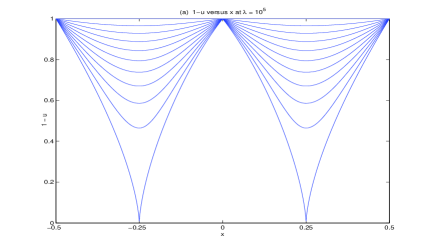
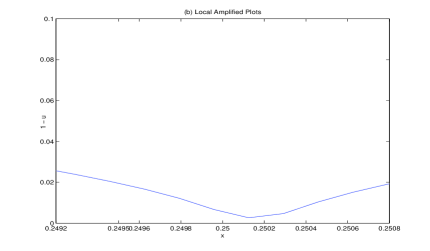
Figure 3: Left figure $(a)$: plots of $1-u$ versus $x$ at different times. Right figure $(b)$: local amplified plots of $(a)$.

Simulation 1. Quenching behavior for small $\lambda>\lambda^{*}$:
In Fig. 2$(a)$: $1-u$ versus $x$ is plotted at different times for $(P)_{\lambda}$ at $\lambda=10$, where the quenching time is $T=0.05174132$. The quenching is observed at $x=\pm 0.204$, a bit far away from the maximum points of profile $f(x)$. In Fig. 2$(b)$: $1-u$ versus $x$ is plotted at different times for $(P)_{\lambda}$ at $\lambda=100$, where the quenching time is $T=0.003523908$. In this case, the quenching is observed at $x=\pm 0.2535$, very close to the maximum points of profile $f(x)$. This simulation shows the necessary of the assumption that Lemma 3.1 and Theorem 3.3 hold only for sufficiently large $\lambda$.

Simulation 2: Quenching behavior for sufficiently large $\lambda$:
In Fig. 3$(a)$, $1-u$ versus $x$ is plotted at different times for $(P)_{\lambda}$ at $\lambda=10^{5}$, where the quenching time is $T=0.000003332783$. In this case, two quenching points are observed at $x=\pm 0.250165$, more close to the maximum points of profile $f(x)$. In Fig. 3$(b)$ we show the local amplified plots of $(a)$ near the maximum point $x=0.25$ of $f(x)$. By further increasing the value of $\lambda$, we observe that quenching points become further close to the maximum points of $f(x)$.

References

[1] H. Brezis, T. Cazenave, Y. Martel, A. Ramiandrisoa, Blow up for
revisited, Adv. Diff. Eqns. (1996), 73–90.
[2] C. Cortazar, M. Elgueta and J. Rossi, The blow-up problem for a semilinear
parabolic equation with a potential, math.AP/0607055.
[3] P. Esposito, N. Ghoussoub and Y. Guo, Compactness along the
branch of semi-stable and unstable solutions for an elliptic problem
with a singular nonlinearity, Comm. Pure Appl. Math. 60
(2007), 1731–1768.
[4]N. Ghoussoub and Y. Guo, On the partial differential equations of electrostatic MEMS
devices: stationary case, SIAM, J. Math. Anal. 38 (2007),
1423–1449.
[5]N. Ghoussoub and Y. Guo, On the partial differential equations of electrostatic MEMS
devices II: dynamic case, NoDEA Nonlinear Diff. Eqns. Appl., in
press 2007.
[6] Y. Guo, On the partial differential equations of electrostatic MEMS
devices III: refined touchdown behavior, J. Diff. Eqns., in press
2007.
[7] Y. Guo, Z. Pan and M. J. Ward, Touchdown and pull-in voltage behavior of a MEMS device with
varying dielectric properties, SIAM, J. Appl. Math. 66
(2005), 309–338.
[8] Y. Giga and R. V. Kohn, Asymptotically self-similar blow-up of semilnear heat
equations, Comm. Pure and Appl. Math. 38 (1985), 297–319.
[9] Y. Giga and R. V. Kohn, Characterizing blow-up using similarity
variables, Indiana Univ. Math. J. 36 (1987), 1–40.
[10] A. A. Lacey, Mathematical analysis of thermal runaway for spatially inhomogeneous reactions,
SIAM J. Appl. Math. 43 (1983), 1350–1366.
[11] J. A. Pelesko, Mathematical modeling of
electrostatic MEMS with tailored dielectric properties, SIAM J.
Appl. Math. 62 (2002), 888–908.
[12] J. A. Pelesko and D. H. Bernstein, Modeling MEMS and NEMS, Chapman Hall and CRC Press, (2002).