Event-Driven Simulation of the Dynamics of Hard Ellipsoids

Abstract

We introduce a novel algorithm to perform event-driven simulations of hard rigid bodies of arbitrary shape, that relies on the evaluation of the geometric distance. In the case of a monodisperse system of uniaxial hard ellipsoids, we perform molecular dynamics simulations varying the aspect-ratio $X_{0}$ and the packing fraction $\phi$. We evaluate the translational $D_{trans}$ and the rotational $D_{rot}$ diffusion coefficient and the associated isodiffusivity lines in the $\phi-X_{0}$ plane. We observe a decoupling of the translational and rotational dynamics which generates an almost perpendicular crossing of the $D_{trans}$ and $D_{rot}$ isodiffusivity lines. While the self intermediate scattering function exhibits stretched relaxation, i.e. glassy dynamics, only for large $\phi$ and $X_{0}\approx 1$, the second order orientational correlator $C_{2}(t)$ shows stretching only for large and small $X_{0}$ values. We discuss these findings in the context of a possible pre-nematic order driven glass transition.

1 Introduction

Particles interacting with only excluded volume interaction may exhibit a rich phase diagram, despite the absence of any attraction. Simple non-spherical hard-core particles can form either crystalline or liquid crystalline ordered phases allenReview, as first shown analytically by Onsager Onsager for rod-like particles. Although detailed phase diagrams of several hard-body (HB) shapes can be found in literature Parsons; Lee2; allenHEPhaseDiag; MargoEvans less detailed information are available about dynamics properties of hard-core bodies and their kinetically arrested states.

The slowing down of the dynamics of the hard-sphere system on increasing the packing fraction $\phi$ is well described by mode coupling theory (MCT) GoetzeMCT, but on going from spheres to non-spherical particles, non-trivial phenomena arise, due to the interplay between translational and rotational degrees of freedom. The slowing down of the dynamics can indeed appear either in both translational and rotational properties or in just one of the two. Hard ellipsoids (HE) of revolution allenReview; singh01 are one of the most prominent systems composed by hard body anisotropic particles.

The equilibrium phase diagram, evaluated numerically two decades ago FrenkelPhaseDiagMolPhys, shows an isotropic fluid phase (I) and several ordered phases (plastic solid, solid, nematic N). The coexistence lines show a swallow-like dependence with a minimum at the spherical limit $X_{0}=1$ and a maximum at $X_{0}\approx 0.5$ and $X_{0}\approx 2$ (cf. Figure 1). Application to HE LetzSchilLatz of the molecular MCT (MMCT) A1ng; A2ng predicts also a swallow-like glass transition line. In addition, the theory suggests that for $X_{0}\lessapprox 0.5$ and $X_{0}\gtrapprox 2$, the glass transition is driven by a precursor of nematic order, resulting in an orientational glass where the translational density fluctuations are quasi-ergodic, except for very small wave vectors $q$. Within MCT, dynamic slowing down associated to a glass transition is driven by the amplitude of the static correlations. Since the approach of the nematic transition line is accompanied by an increase of the nematic order correlation function at $q=0$, the non-linear feedback mechanism of MCT results in a glass transition, already before macroscopic nematic order occurs LetzSchilLatz. In the arrested state, rotational motions become hindered.

We perform event-driven (ED) molecular dynamics simulations, using a new algorithm DeMicheleHEJCP; DeMichelePRL2007, that differently from previous ones AllenFrenkelDyn; DonevTorqStill1, relies on the evaluation of the distance between objects of arbitrary shape and that will be illustrated shortly.

The outline of the manuscript is as follows. In the next section we illustrate shortly the new algorithm, that we proposed for simulating objects of arbitrary shape. Then in Sec. 3 we illustrate the model used and we give all the details of the simulations we performed. In Sec. 4 we show the results concerning the dynamics of the system investigated. The final section contains our conclusions.

2 Algorithm details

2.1 An event-driven algorithm for hard rigid bodies

In an ED simulation the system is propagated until the next event occurs, where an event can be a collision between particles, a cell crossing (if linked lists are used), etc. All these events must be ordered with respect to time in a calendar and insertion, deletion and retrieving of events must be performed as efficiently as possible.

One elegant approach has been introduced twenty years ago by Rapaport RapaBook, who proposed to arrange all events into an ordered binary tree (that is the calendar of events), so that insertion, deletion and retrieving of events can be done with an efficiency $O(\log N)$, $O(1)$ and $O(\log N)$ respectively, where $N$ is the number of events in the calendar. We adopt this solution to handle the events in our simulation; all the details of this method can be found in RapaBook. Our ED algorithm can be schematized, as follows:

1. Initialize the events calendar (predict collisions, cells crossings, etc.).

2. Retrieve next event $\cal E$ and set the simulation time to the time of this event.

3. If the final time has been reached, terminate.

4. If $\cal E$ is a collision between particles $A$ and $B$ then:

   1. change angular and center-of-mass velocities of $A$ and $B$ (see DonevTorqStill2).

   2. remove from the calendar all the events (collisions, cell-crossings) in which $A$ and $B$ are involved.

   3. predict and schedule all possible collisions for $A$ and $B$.

   4. predict and schedule the two cell crossings events for $A$ and $B$.

5. If $\cal E$ is a cell crossing of a certain rigid body $A$:

   1. update linked lists accordingly.

   2. remove from calendar all events (collisions, cell-crossings) in which $A$ is involved.

   3. predict and schedule all possible collisions for $A$ using the updated linked lists.

6. go to step 2.

All the details about linked lists can be found again in Ref. RapaBook, where an ED algorithm for hard spheres is illustrated. We note also that in the case of HE, according to DonevTorqStill2, if the elongation of HE is big (i.e. one axes is much greater or much smaller than the others), the linked list method becomes inefficient at moderate and high densities. In fact, given one ellipsoid $A$, using the linked lists, collision times of $A$ with all ellipsoids in the same cell of $A$ and with all the $26$ adjacent cells have to be predicted. In the case of rotationally symmetric ellipsoids, the number of time-of-collision predictions grows as $X_{0}^{2}$, if $X_{0}>1$ and as $X_{0}$, if $X_{0}<1$ DonevTorqStill2. To overcome this problem, we developed also a new nearest neighbours list (NNL) method. At the begin of the simulation we build an oriented bounding parallelepiped (OBP) around each ellipsoid and we only predict collisions between ellipsoids having overlapping OBP. In other words given an ellipsoid $A$, all the ellipsoids having overlapping OBP are the NNL of $A$. In addition the time-of-collisioni $t_{i}$ of each ellipsoid with its corresponding OBP is evaluated and the NNL of each HE is rebuilt at the time $t=\min_{i}\{t_{i}\}$. The most time-consuming step in the case of hard rigid bodies is the prediction of collisions between HE, hence in the following a short description of the algorithm, that we developed, is given.

2.2 Distance between two rigid bodies

Our algorithm for predicting the collision time of two rigid bodies relies on the evaluation of the distance between them. The surfaces of two rigid bodies, $A$ and $B$, are implicitly defined by the following equations:

$$f({\bf x})=0$$ (1a)

$$g({\bf x})=0$$ (1b)

In passing we note that in the case of uniaxial hard ellipsoids, we have $f({\bf x},t)={}^{t}({\bf x}-{\bf r}_{A}(t))X_{A}(t)({\bf x}-{\bf r}_{A}(t))-1$ and a similar expression holds for $g({\bf x})$, where ${\bf r}_{A}$ is the position of the center-of-mass of $A$ and $X_{A}(t)$ is a matrix, that depends on the orientation of the $A$ (see DonevTorqStill2). It is assumed that, if a point ${\bf x}$ is inside the rigid body $A$ ($B$), then $f({\bf x})<0$ ($g({\bf x})<0$), while if it is outside $f({\bf x})>0$ ($g({\bf x})>0$). Then the distance $d$ between these two objects can be defined as follows:

$$d=\min_{\genfrac{}{}{0.0pt}{}{f({\bf x}_{A})=0}{g({\bf x}_{B})=0}}\|{\bf x}_{A}-{\bf x}_{B}\|$$ (2)

Equivalently, the distance between these two objects can be defined as the solution of the following set of equations:

$$f_{{\bf x}_{A}}=-\alpha^{2}g_{{\bf x}_{B}}$$ (3a)

$$f({\bf x}_{A})=0$$ (3b)

$$g({\bf x}_{B})=0$$ (3c)

$${\bf x}_{A}+\beta f_{{\bf x}_{A}}={\bf x}_{B}$$ (3d)

where ${\bf x}_{A}=(x_{A},y_{A},z_{A})$, ${\bf x}_{B}=(x_{B},y_{B},z_{B})$, $f_{{\bf x}_{A}}=\frac{\partial f}{\partial{\bf x}_{A}}$ and $g_{{\bf x}_{B}}=\frac{\partial f}{\partial{\bf x}_{B}}$. Eqs. (3b) and (3c) ensure that ${\bf x}_{A}$ and ${\bf x}_{B}$ are points on $A$ and $B$, eq.(3a) provides that the normals to the surfaces are anti-parallel, and eq.(3d) ensures that the displacement of ${\bf x}_{A}$ from ${\bf x}_{B}$ is collinear to the normals of the surfaces. Equations (3) define extremal points of $d$; therefore, for two general HB these equations can have multiple solutions, while only the smallest one is the actual distance. To solve such equations iteratively is therefore necessary to start from a good initial guess of $\left({\bf x}_{A},{\bf x}_{B},\alpha,\beta\right)$ to avoid finding spurious solutions.

In addition note that if two HB overlap slightly (i.e. the overlap volume is small) there is a solution with $\beta<0$ that is a measure of the inter-penetration of the two rigid bodies; we will refer to such a solution as the “negative distance” solution.

2.2.1 Newton-Raphson method for the distance

The set of equations (3) can be conveniently solved by a Newton-Raphson (NR) method, as long as first and second derivatives of $f({\bf x}_{A})$ and $g({\bf x}_{B})$ are well defined. This method, provided that a good initial guess has been supplied, very quickly reaches the solution because of its quadratic convergence NumRecipes. If we define:

$${\bf F}({\bf y})=\begin{pmatrix}f_{{\bf x}_{A}}+\alpha^{2}g_{{\bf x}_{B}}\cr f({\bf x}_{A})\cr g({\bf x}_{B})\cr{\bf x}_{A}+\beta f_{{\bf x}_{A}}-{\bf x}_{B}\end{pmatrix}$$ (4)

Eqs. (3) become:

$$\ {\bf F}({\bf y})=0$$ (5)

where ${\bf y}=({\bf x}_{A},{\bf x}_{B},\alpha,\beta)$.

Given an initial point ${\bf y}_{0}$ we build a sequence of points converging to the solution as follows:

$${\bf y}_{i+1}={\bf y}_{i}+{\bf J}^{-1}{\bf F}({\bf y}_{i})$$ (6)

where ${\bf J}$ is the Jacobian of ${\bf F}$,i.e. ${\bf J}=\frac{\partial\bf F}{\partial\bf y}$.

The matrix inversion, required to evaluate ${\bf J}^{-1}$, can be done making use of a standard $LU$ decomposition NumRecipes. This decomposition is of order $N^{3}/3$, where is $N$ the number of equations ($8$ in the present case). Finally we note that the set of $8$ equations (3) can be also reduced to $5$ equations, eliminating ${\bf x}_{A}$ or ${\bf x}_{B}$, using Eq. (3d) .

2.3 Prediction of the time-of-collision

The collision (or contact) time of two rigid bodies $A$ and $B$ is, the smallest time $t_{c}$, such that $d(t_{c})=0$, where $d(t)$ is the distance as a function of time between $A$ and $B$. For finding $t_{c}$ we perform the following steps:

1. Bracket the contact time using centroids (this technique will not be discussed here, see DonevTorqStill1; DonevTorqStill2 for the details)

2. Overestimating the rate of variation of the distance with respect to time ($\dot{d}(t)$), refine the bracketing of the collision time obtained in $1$.

3. Find the collision time to the best accuracy using a Newton-Raphson on a suitable set of equations for the contact point and the contact time.

2.3.1 Bracketing of the contact time overestimating $\dot{d}(t)$.

It can be proved that an overestimate of the rate of variation of the distance is the following:

$$\dot{d}(t)\leq\|{\bf v}_{A}-{\bf v}_{B}\|+\|{\bf w}_{A}\|L_{A}+\|{\bf w}_{B}\|L_{B}$$ (7)

where the dot indicates the derivation with respect to time, ${\bf r}_{A}$ and ${\bf r}_{B}$ are the centers of mass of the two rigid bodies, ${\bf v}_{A}$ and ${\bf v}_{B}$ are the velocities of the centers of mass, and the lengths $L_{A}$, $L_{B}$ are such that

$$L_{A}\geq\max_{{f({\bf r}^{\prime})\leq 0}}\{\|{\bf r}^{\prime}-{\bf r}_{A}\|\}$$ (8a)

$$L_{B}\geq\max_{{g({\bf r}^{\prime})\leq 0}}\{\|{\bf r}^{\prime}-{\bf r}_{B}\|\}$$ (8b)

Using this overestimate of $\dot{d}(t)$, that will be called $\dot{d}_{max}$ from now on, an efficient strategy, to refine the bracketing of the contact time, is the following:

1. If $t_{1}$ and $t_{2}$ bracket the solution, set $t=t_{1}$.

2. Evaluate the distance $d(t)$ at time $t$.

3. Choose a time increment $\Delta t$ as follows:

   $$\Delta t=\begin{cases}\frac{d(t)}{\dot{d}_{max}},&\hbox{if}\>d(t)>\epsilon_{d}\hbox{;}\cr\frac{\epsilon_{d}}{\dot{d}_{max}},&\hbox{otherwise.}\cr\end{cases}$$ (9)

   where $\epsilon_{d}\ll\min\{L_{A},L_{B}\}$

4. Evaluate the distance at time $t+\Delta t$.

5. If $d(t+\Delta t)<0$ and $d(t)>0$, then $t_{1}=t$ and $t_{2}=t+\Delta t$, find the collision time/point via NR (see Sec. 2.3.2) and terminate (collision will occur after $t_{1}$).

6. if both $0<d(t+\Delta t)<\epsilon_{d}$ and $0<d(t)<\epsilon_{d}$, there could be a “grazing“ collision between $t$ and $t+\Delta t$ DonevTorqStill2 (distance is first decreasing and then increasing). To look for a possible collision, evaluate the distance $d(t+\Delta t/2)$ and perform a quadratic interpolation of the $3$ points ( $(t,d(t))$, $(t+\Delta t/2,d(t+\Delta t/2)$, $(t+\Delta t,d(t+\Delta t)$ ). If the resulting parabola has zeros, set $t_{1}$ to the smallest zero (first collision will occur near the smallest zero), and find the collision time/point via NR and terminate (see Sec. 2.3.2).

7. Increment time by $t\rightarrow t+\Delta t$.

8. if $t>t_{2}$ terminate (no collision has been found).

9. Go to step 2.

Finally we note that if the quadratic interpolation fails, the collision will be missed, anyway if $\epsilon_{d}$ is enough small all “grazing“ collisions will be properly handled, i.e. all collisions will be correctly predicted.

2.3.2 Set of equations to find the contact time and the contact point

The contact time, to the best possible accuracy, can be found solving the following equations:

$$f_{{\bf x}}({\bf x},t)=-\alpha^{2}g_{{\bf x}}({\bf x},t)$$ (10a)

$$f({\bf x},t)=0$$ (10b)

$$g({\bf x},t)=0$$ (10c)

where now $f$ and $g$ depend also on time because the two objects move, and the independent variables are the contact time and the contact point. Again, a good way to solve such a system is using the NR method, very similarly to what we did for evaluating the geometric distance. NR for Eqs. (10) is again very unstable unless a very good initial guess is provided, but the bracketing evaluated using $\dot{d}_{max}$ is sufficiently accurate, provided that $\epsilon_{d}$ is enough small (typically $\epsilon_{d}\lessapprox 1E-4$ is a good choice to give a good initial guess for this NR and to avoid “grazing“ collisions).

Finally we want to stress that this algorithm will be exploited fully, when hard bodies of arbitrary shape will be simulated, and that with minor changes it can also be used to simulate hard bodies decorated with attractive spots, as it has been done in the past for the specific case of hard-spheres DeMicheleH2O; DeMicheleSiO2. Work along these directions is on the way, and in particular a system of super-ellipsoids has been already successfully simulated using the present algorithm.

3 Methods

We perform an extended study of the dynamics of monodisperse HE in a wide window of $\phi$ and $X_{0}$ values, extending the range of $X_{0}$ previously studied AllenFrenkelDyn. We specifically focus on establishing the trends leading to dynamic slowing down in both translations and rotations, by evaluating the loci of constant translational and rotational diffusion. These lines, in the limit of vanishing diffusivities, approach the glass-transition lines. We also study translational and rotational correlation functions, to search for the onset of slowing down and stretching in the decay of the correlation. We simulate a system of $N=512$ ellipsoids at various volumes $V=L^{3}$ in a cubic box of edge $L$ with periodic boundary conditions. We chose the geometric mean of the axis $l=\sqrt[3]{ab^{2}}$ as unit of distance, the mass $m$ of the particle as unit of mass ($m=1$) and $k_{B}T=1$ (where $k_{B}$ is the Boltzmann constant and $T$ is the temperature) and hence the corresponding unit of time is $\sqrt{ml^{2}/k_{B}T}$. The inertia tensor is chosen as $I_{x}=I_{y}=2mr^{2}/5$, where $r=\min\{a,b\}$. The value of the $I_{z}$ component is irrelevant allenfrenkelBook, since the angular velocity along the symmetry (z-) axis of the HE is conserved. We simulate a grid of more than 500 state points at different $X_{0}$ and $\phi$.To create the starting configuration at a desired $\phi$, we generate a random distribution of ellipsoids at very low $\phi$ and then we progressively decrease $L$ up to the desired $\phi$. We then equilibrate the configuration by propagating the trajectory for times such that both angular and translational correlation functions have decayed to zero. Finally, we perform a production run at least $30$ times longer than the time needed to equilibrate. For the points close to the I-N transition we check the nematic order by evaluating the largest eigenvalue $S$ of the order tensor ${\bf Q}$ SpheroCylRec, whose components are:

$$Q_{\alpha\beta}=\frac{3}{2}\frac{1}{N}\sum_{i}\langle({\bf u}_{i})_{\alpha}({\bf u}_{i})_{\beta}\rangle-\frac{1}{3}\delta_{\alpha,\beta}$$ (11)

where $\alpha\beta\in\{x,y,z\}$, and the unit vector $({\bf u}_{i}(t))_{\alpha}$ is the component $\alpha$ of the orientation (i.e. the symmetry axis) of ellipsoid $i$ at time $t$. The largest eigenvalue $S$ is non-zero if the system is nematic and $0$ if it is isotropic. In the following, we choose the value $S=0.3$ as criteria to separate isotropic from nematic states.

4 Results and discussion

4.1 Isodiffusivity lines

From the grid of simulated state points we build a corresponding grid of translational ($D_{trans}$) and diffusional ($D_{rot}$) coefficients, defined as:

$$D_{trans}=\lim_{t\rightarrow+\infty}\frac{1}{N}\sum_{i}\frac{\langle\|{\bf x}_{i}(t)-{\bf x}_{i}(0)\|^{2}\rangle}{6t}$$ (12)

$$D_{rot}=\lim_{t\rightarrow+\infty}\frac{1}{N}\sum_{i}\frac{\langle\|\Delta\Phi_{i}\|^{2}\rangle}{4t}$$ (13)

where $\Delta\Phi_{i}=\int_{0}^{t}{\bf\omega}_{i}dt$, ${\bf x}_{i}$ is the position of the center of mass and ${\bf\omega}_{i}$ is the angular velocity of ellipsoid $i$. By proper interpolation, we evaluate the isodiffusivity lines, shown in Fig. 1. Results show a striking decoupling of the translational and rotational dynamics. While the translational isodiffusivity lines mimic the swallow-like shape of the coexistence between the isotropic liquid and the crystalline phases (as well as the MMCT prediction for the glass transition LetzSchilLatz), rotational isodiffusivity lines reproduce qualitatively the shape of the I-N coexistence. As a consequence of the the swallow-like shape, at large fixed $\phi$, $D_{trans}$ increases by increasing the particle’s anisotropy, reaching its maximum at $X_{0}\approx 0.5$ and $X_{0}\approx 2$. Further increase of the anisotropy results in a decrease of $D_{trans}$. For all $X_{0}$, an increase of $\phi$ at constant $X_{0}$ leads to a significant suppression of $D_{trans}$, demonstrating that $D_{trans}$ is controlled by packing. The iso-rotational lines are instead mostly controlled by $X_{0}$, showing a progressive slowing down of the rotational dynamics independently from the translational behavior. This suggests that on moving along a path of constant $D_{trans}$, it is possible to progressively decrease the rotational dynamics, up to the point where rotational diffusion arrest and all rotational motions become hindered. Unfortunately, in the case of monodisperse HE, a nematic transition intervenes well before this point is reached. It is thus stimulating to think about the possibility of designing a system of hard particles in which the nematic transition is inhibited by a proper choice of the disorder in the particle’s shape/elongations. We note that the slowing down of the rotational dynamics is consistent with MMCT predictions of a nematic glass for large $X_{0}$ HE LetzSchilLatz, in which orientational degrees of freedom start to freeze approaching the isotropic-nematic transition line, while translational degrees of freedom mostly remain ergodic.

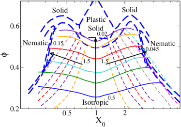
Figure 1: [Color online] Isodiffusivity lines. Solid lines are isodiffusivity lines from translational diffusion coefficients $D_{trans}$ and dashed lines are isodiffusivities lines from rotational diffusion coefficients $D_{rot}$. Arrows indicate decreasing diffusivities. Left and right arrows refer to rotational diffusion coefficients. Diffusivities along left arrow are: $1.5$, $0.75$, $0.45$, $0.3$, $0.15$. Diffusivities along right arrow are: $1.5$, $0.75$, $0.45$, $0.3$, $0.15$, $0.075$, $0.045$. Central arrow refers to translational diffusion coefficients, whose values are: $0.5$, $0.3$, $0.2$, $0.1$, $0.04$, $0.02$. Thick Long-dashed curves are coexistence curves of all first order phase transitions in the phase diagram of HE evaluated by Frenkel and Mulder (FM) FrenkelPhaseDiagMolPhys Solid lines are coexistence curves for the I-N transition of oblate and prolate ellipsoids, obtained analytically by Tijpto-Margo and Evans MargoEvans (TME).

4.2 Orientational correlation function

To support the possibility that the slowing down of the dynamics on approaching the nematic phase originates from a close-by glass transition, we evaluate the self part of the intermediate scattering function $F_{self}(q,t)=\frac{1}{N}\langle\sum_{j}e^{i{\bf q}\cdot({\bf x}_{j}(t)-{\bf x}_{j}(0))}\rangle$ and the second order orientational correlation function $C_{2}(t)$ defined as AllenFrenkelDyn $C_{2}(t)=\langle P_{2}(\cos\theta(t))\rangle$, where $P_{2}(x)=(3x^{2}-1)/2$ and $\theta(t)$ is the angle between the symmetry axis at time $t$ and at time $0$. The $C_{2}(t)$ rotational isochrones are found to be very similar to rotational isodiffusivity lines.

These two correlation functions never show a clear two-step relaxation decay in the entire studied region, even where the isotropic phase is metastable, since the system can not be significantly over-compressed. As for the well known hard-sphere case, the amount of over-compressing achievable in a monodisperse system is rather limited. This notwithstanding, a comparison of the rotational and translational correlation functions reveals that the onset of dynamic slowing down and glassy dynamics can be detected by the appearance of stretching.

We note that $F_{self}$ shows an exponential behaviour close to the I-N transition ($X_{0}=3.2$,$\ 0.3448$) on the prolate and oblate side, in agreement with the fact that translational isodiffusivities lines do not exhibit any peculiar behaviour close to the I-N line DeMichelePRL2007. Only when $X_{0}\approx 1$, $F_{self}$ develops a small stretching, consistent with the minimum of the swallow-like curve observed in the fluid-crystal line HardSpheresExp; HardSpheresSim, in the jamming locus as well as in the predicted behavior of the glass line for HE LetzSchilLatz and for small elongation dumbbells DumbellChongGoetze; DumbellChongFra. Opposite behavior is seen for the case of the orientational correlators. $C_{2}$ shows stretching at large anisotropy, i.e. at small and large $X_{0}$ values, but decays within the microscopic time for almost spherical particles. In this quasi-spherical limit, the decay is well represented by the decay of a free rotator FreeRotator; DeMichelePRL2007. Previous studies of the rotational dynamics of HE AllenFrenkelDyn did not report stretching in $C_{2}$, probably due to the smaller values of $X_{0}$ previously investigated and to the present increased statistic which allows us to follow the full decay of the correlation functions.

In summary $C_{2}$ becomes stretched approaching the I-N transition while $F_{self}$ remains exponential on approaching the transition. To quantify the amount of stretching in $C_{2}$, we fit it to the function $A\exp[-(t/\tau_{C_{2}})^{\beta_{C_{2}}}]$ (stretched exponential) for several state points and we show in Fig. 2 the $X_{0}$ dependence of $\tau_{C_{2}}$ and $\beta_{C_{2}}$ for three different values of $\phi$. In all cases, slowing down of the characteristic time and stretching increases progressively on approaching the I-N transition.

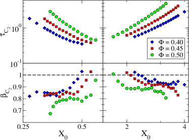
Figure 2: [Color online] $\beta_{C_{2}}$ and $\tau_{C_{2}}$ are obtained from fits of $C_{2}$ to a stretched exponential for $\phi=0.40,0.45$ and $0.50$. Top: $\tau_{C_{2}}$ as a function of $X_{0}$. Bottom: $\beta_{C_{2}}$ as a function of $X_{0}$. The time window used for the fits is chosen in such a way to exclude the microscopic short times ballistic relaxation. For $0.588<X_{0}<1.7$ the orientational relaxation is exponential.

5 Conclusions

In summary we have applied a novel algorithm for simulating hard bodies to investigate the dynamics properties of a system of monodisperse HE and we have shown that clear precursors of dynamic slowing down and stretching can be observed in the region of the phase diagram where a (meta)stable isotropic phase can be studied. Despite the monodisperse character of the present system prevents the possibility of observing a clear glassy dynamics, our data suggest that a slowing down in the orientational degrees of freedom — driven by the elongation of the particles — is in action. The main effect of this shape-dependent slowing down is a decoupling of the translational and rotational dynamics which generates an almost perpendicular crossing of the $D_{trans}$ and $D_{rot}$ isodiffusivity lines. This behavior is in accordance with MMCT predictions, suggesting two glass transition mechanisms, related respectively to cage effect (active for $0.5\lessapprox X_{0}\lessapprox 2$) and to pre-nematic order ($X_{0}\lessapprox 0.5$, $X_{0}\gtrapprox 2$) LetzSchilLatz.