A geometric theory of swimming: Purcell’s swimmer and its symmetrized cousin

Abstract

We develop a qualitative geometric approach to swimming at low Reynolds number which avoids solving differential equations and uses instead landscape figures of two notions of curvatures: The swimming curvature and the curvature derived from dissipation. This approach gives complete information for swimmers that swim on a line without rotations and gives the main qualitative features for general swimmers that can also rotate. We illustrate this approach for a symmetric version of Purcell’s swimmer which we solve by elementary analytical means within slender body theory. We then apply the theory to derive the basic qualitative properties of Purcell’s swimmer.

1 Introduction

Micro-swimmers are of general interest lately, motivated by both engineering and biological problems [9, 6, 16, 3, 7, 4, 8, 1, 11, 17]. They can be remarkably subtle as was illustrated by E. M. Purcell in his famous talk on “Life at low Reynolds numbers” [13] where he introduced a deceptively simple swimmer shown in Fig. 1. Purcell asked “What will determine the direction this swimmer will swim?” This simple looking question took 15 years to answer: Koehler, Becker and Stone [3] found that the direction of swimming depends, among other things, on the stroke’s amplitude: Increasing the amplitudes of certain small strokes that propagate the swimmer to the right result in propagation to the left. This shows that even simple qualitative aspects of low Reynolds number swimming can be quite un-intuitive.

Purcell’s swimmer made of three slender rods can be readily analyzed numerically by solving three coupled, non-linear, first order, differential equations [16]. However, at present there appears to be no general method that can be used to gain direct qualitative insight into the properties of the solutions of these equations.

Our first aim here is to to describe a geometric approach which allows one to describe the qualitative features of the solution of the swimming differential equations without actually solving them. Our tools are geometric. The first tool is the notion of curvature borrowed from non-Abelian gauge theory [18]. This curvature can be represented graphically by landscape diagrams such as Figs. 3,5,8 which capture the qualitative properties of general swimming strokes. We have taken care not to assume any pre-existing knowledge about gauge theory on part of the reader. Rather, we have attempted to use swimming as a natural setting where one can build and develop a picture of the notions of non-Abelian gauge fields. Purcell’s original question, “What will determine the direction this swimmer will swim?” can often be answered by simply looking at such landscape pictures.

Our second tool is a notion of metric and curvature associated with the dissipation. The “dissipation curvature” can be described as a landscape diagram and it gives information on the geometry of “shape space”. This gives us useful geometric tools that give qualitative information on the solutions of rather complicated differential equations.

We begin by illustrating these geometric methods for the symmetric version of Purcell’s swimmer, shown in Fig. 2. Symmetry protects the swimmer against rotations so it can only swim on a straight line. This makes it simple to analyze by elementary analytical means. In particular, it is possible to predict, using the landscape portraits of the swimming curvature Fig. 3, which way it will swim. In this (Abelian) case the swimming curvature gives full quantitative information on the swimmer. We then turn to the non-Abelian case of the usual Purcell’s swimmer which can also rotate. There are now several notions of swimming curvatures: The rotation curvature and the two translation curvature. The translation curvatures are non-Abelian. This means that they give precise information of small strokes but this information can not be integrated to learn about large strokes. This can be viewed as a failure of Stokes integration theorem. Nevertheless, as we shall explain, they do give lots of qualitative information about large strokes as well.

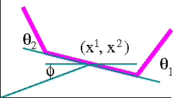
Figure 1: Purcell’s swimmer. The swimmer controls the angles $|\theta_{1,2}|<\pi$. The location of the swimmer in the plane is determined by two position coordinates $x^{1,2}$ and one orientation $x^{0}=\phi$. The lengths of each arm is $\ell$ and the length of the body $\ell_{0}$.

2 The symmetric Purcell’s swimmer

Purcell’s swimmer, which was invented as “The simplest animal that can swim that way” [13], is not simple to analyze. A variant of it that is simple to analyze is shown in the Fig  2.

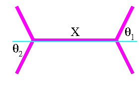
Figure 2: The symmetrized Purcell’s swimmer can not rotate and can only move along the horizontal body-axis. The length of each arm is $\ell$ and the length of the body $\ell_{0}$. The position of the swimmer is denoted by $X$.

The swimmer has four arms, each of length $\ell>0$ and one body arm of length $\ell_{0}$, (possibly of zero length). The swimmer can control the angles $\theta_{j}$ and the arms are not allowed to touch. Both angles increase in the counterclockwise direction, $0<\theta_{j}<\pi$.

Being symmetric, this swimmer can not rotate and can swim only in the “body” direction. It falls into the class of “simple swimmers” which includes the “three linked spheres” of Najafi and Glolestanian [9] and the Pushmepullyou [1], whose hydrodynamics is elementary because they can not turn.

Let us first address Purcell’s question “What will determine the direction this swimmer will swim?” for the stroke shown in Fig. 3. In the stroke, the swimmer moves the two arms backwards together and then bring them forward one by one. The first half of the cycle pushes the swimmer forward and the second half pulls it back. Which half of the cycle wins?

To answer that, one needs to remember that swimming at low Reynolds numbers relies more on effective anchors than on good propellers. Since one needs twice the force to drag a rod transversally than to drag it along its axis [10], an open arm $\theta_{j}\approx\pi/2$ acts like an anchor. This has the consequence that rowing with both arms, in the same direction and in phase, is less effective than bringing them back out of phase. The stroke actually swims backwards. This reasoning also shows that the swimmer is Sisyphian: it performs a lot of forward and backward motion for little net gain.

The swimming equation

The swimming equation at low Reynolds number is the requirement that the total force (and torque) on the swimmer is zero. The total force (and torque) is the sum of the forces (and torques) on the four arms and body. For the symmetric swimmer, the torque and force in the transversal direction vanish by symmetry. The swimming equation is the condition that the force in the body-direction vanishes. This force depends linearly on the known rate of change of the controls, $\dot{\theta}$ and the unknown the velocity $\dot{X}$ of the “body-rod”. It gives a linear equation for the velocity.

For slender arms and body, the forces are given by Cox [5] slender body theory: The element of force, $d\mathbf{F}(s)$, acting on a segment of length $ds$ located at the point $s$ on the slender body is given by

$$d\mathbf{F}(s)=k\big{(}\mathbf{t}\big{(}\mathbf{t}\cdot\mathbf{v}\big{)}-2\mathbf{v}\big{)}\,ds,\quad k=\frac{2\pi\mu}{\ln\kappa}$$ (2.1)

where $\mathbf{t}(s)$ is a unit tangent vector to the slender-body at $s$ and $\mathbf{v}(s)$ its velocity there. $\mu$ is the viscosity and $\kappa$ the slenderness (the ratio of length to diameter).

The force on the a-th arm depends linearly on the velocities of the controls $\dot{\theta}_{j}$ and swimming velocity $\dot{X}$. For example, the force component in the x-direction on the a-th arm takes the form

$${F}_{a}^{x}=f_{aj}^{x}\,\dot{\theta}_{j}+f_{a}^{xx}\,\dot{X}$$ (2.2)

where $f_{aj}^{x}$ are functions of the controls, given by elementary integrals

$$f_{a}^{xx}=k(\cos^{2}\theta_{a}-2)\int_{0}^{\ell}ds\,,\quad f_{aj}^{x}=2k\sin\theta_{j}\,\int_{0}^{\ell}s\,ds$$ (2.3)

Similar equations hold for the left arm and the body. The requirement that the total force on the swimmer vanishes gives a linear relation between the variation of the controls and the displacement $\kern-1.00006pt{\raise 3.44444pt\hbox{ -}}\kern-6.00006pt{d}x$

$$\kern-1.00006pt{\raise 3.44444pt\hbox{ -}}\kern-6.00006pt{d}x=\frac{\kern-1.00006pt{\raise 3.44444pt\hbox{ -}}\kern-6.00006pt{d}X}{\ell}=-a(\xi,\eta)\,(d\xi_{1}+d\xi_{2}),\quad\xi_{j}=\cos\theta_{j},$$ (2.4)

where

$$a(\xi,\eta)=\frac{1}{4+\eta-\xi_{1}^{2}-\xi_{2}^{2}},\quad\eta=\frac{\ell_{0}}{2\ell}$$ (2.5)

As one expects, the body is just a “dead weight” and a trim swimmer with $\eta=0$ is best.

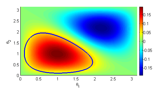
Figure 3: The swimming curvature (measured in the dissipation metric) on the surface of controls for the symmetric Purcell swimmer. The closed curve shows the optimal stroke. A bona fide optimizer exists since the swimming curvature vanishes on the boundary $\theta_{j}=\pi,0$ .

The curvature

The notation $\kern-1.00006pt{\raise 3.44444pt\hbox{ -}}\kern-6.00006pt{d}x$ stresses that the differential displacement does not integrate to a function of the controls, $x(\xi)$. This is the essence of swimming: $x$ fails to return to its original value with $\xi$. For this reason, swimming is best captured not by the differential one-form $\kern-1.00006pt{\raise 3.44444pt\hbox{ -}}\kern-6.00006pt{d}x$ but by the differential two-form $\mathcal{F}=d\kern-1.00006pt{\raise 3.44444pt\hbox{ -}}\kern-6.00006pt{d}x$

$$\mathcal{F}=d\kern-1.00006pt{\raise 3.44444pt\hbox{ -}}\kern-6.00006pt{d}x=2a^{2}(\xi,\eta)(\xi_{2}-\xi_{1})\,d\xi_{1}\wedge d\xi_{2}$$ (2.6)

and $a(\xi)$ is the rational function given in Eq. (2.5). $\mathcal{F}$ is commonly known as the curvature [18] and its surface integral for a region enclosed by a curve $\gamma$ gives, by Stokes, the distance covered in one stroke. It gives complete information on both the direction of swimming and distance.

The total curvature associated with the full square of shape space, $|\xi_{j}|\leq 1$ is 0 by symmetry. The total positive curvature associated with the triangular half of the square, $\xi_{1}\leq\xi_{2}$ is 0.274. This means that swimmer can swim, at most, about a quarter of its arms length in a single stroke.

$\mathcal{F}$ is a differential two form and as such is assigned a numerical value only when in comes with a region of integration. By itself, it has no numerical value. To say that the curvature is large at a given point in shape, or control, space requires fixing some a-priori measure. For example one can pick the flat measure for $\xi$ in which case $a^{2}(\xi,\eta)(\xi_{1}-\xi_{2})$ gives numerical values for the curvature. However, one can pick instead the flat measure for $\theta$ one gets a different function. A natural measure on shape space is determined by the dissipation. We turn to it now.

The metric in shape space

The power of swimming at low Reynolds numbers is quadratic in the driving: $g_{jk}\,\dot{\theta}_{j}\dot{\theta}_{k}$ where $g_{jk}(\theta)$ is a function on shape space and we use the summation convention where repeated indices are summed over. This suggests the natural metric in shape space is, in either coordinate systems,

$$g_{jk}(\theta)\,d\theta_{j}d\theta_{k}=g_{jk}(\xi)\,d\xi_{j}d\xi_{k}$$ (2.7)

In particular, the associated area form is

$$\sqrt{\det g(\theta)}\,d\theta_{1}\wedge d\theta_{2}=\sqrt{\det g(\xi)}\,d\xi_{1}\wedge d\xi_{2}$$ (2.8)

The curvature can now be assigned a natural numerical value

$$2a^{2}(\xi,\eta)\frac{\xi_{1}-\xi_{2}}{\sqrt{\det g(\xi)}}=2a^{2}(\xi,\eta)\frac{\xi_{1}-\xi_{2}}{\sqrt{\det g(\theta)}}\sin\theta_{1}\sin\theta_{2}$$ (2.9)

Each arm of the symmetric Purcell swimmer dissipate energy at the rate

$$-\int_{0}^{\ell}d\mathbf{F}(s)\cdot\mathbf{v}ds = -k\int_{0}^{\ell}\big{(}(\mathbf{t}\cdot\mathbf{v})^{2}-2\mathbf{v}\cdot\mathbf{v}\big{)}\,ds$$

$$= -k\int_{0}^{\ell}\big{(}\dot{X}^{2}-2s^{2}\dot{\theta}_{j}^{2}\cos^{2}\theta_{j}-2(s\dot{\theta}_{j}\,\sin\theta_{j}-\dot{X})^{2}\big{)}\,ds$$

$$= \frac{k\ell^{3}}{3}\left(3\dot{x}^{2}+2\dot{\theta}_{j}^{2}+6\dot{\xi}_{j}\dot{x}\right)$$

And the total energy dissipation by the arms is evidently

$$\frac{2k\ell^{3}}{3}\left(6\dot{x}^{2}+2(\dot{\theta}_{1}^{2}+\dot{\theta}_{2}^{2})+6(\dot{\xi}_{1}+\dot{\xi}_{2})\dot{x}\right)$$ (2.11)

In a body-less swimmer, $\eta=0$, this is also the total dissipation, and we consider this case from now on. Since we are interested in the metric up to units, we shall henceforth set $4k\ell^{3}=3$. Plugging the swimming equation, Eq. (2.4) gives $g$:

$$g(\theta)=a(\xi,0)\left(\begin{array}[]{cc}5-2\xi_{2}^{2}+\xi_{1}^{2}&\sin\theta_{1}\sin\theta_{2}\\ \sin\theta_{1}\sin\theta_{2}&5-2\xi_{1}^{2}+\xi_{2}^{2}\\ \end{array}\right),\quad\xi_{j}=\cos\theta_{j}$$ (2.14)

and $a(\xi,0)$ is given in Eq. (2.5). In particular, $g(\theta)$ is a smooth function on shape space while $g(\xi)$ is singular at the boundaries. One can now meaningfully plot the curvature which is shown in Fig. 3

The optimal stroke

Efficient swimming covers the largest distance for given energy resource and at a given speed. Alternatively, it minimizes the energy needed for covering a given distance at a given speed. Fixing the speed for a given distance is equivalent to fixing the time $\tau$. In this formulation the variational problem takes the form of a problem in Lagrangian mechanics of minimizing the action

$$\int\limits_{0}\limits^{\tau}g_{jk}(\theta)\,\dot{\theta}_{j}\dot{\theta}_{k}dt+q\int\kern-1.00006pt{\raise 3.44444pt\hbox{ -}}\kern-6.00006pt{d}x$$ (2.15)

where q is a Lagrange multiplier. $\kern-1.00006pt{\raise 3.44444pt\hbox{ -}}\kern-6.00006pt{d}x$ is given in Eq. (2.4). This can be interpreted as a motion of a a charged particle on a curved surface in an external magnetic field [2]. Conservation of energy then says that the solution has constant speed (in the metric $g$). For a closed path, the kinetic term is then proportional to the length of the path and the constraint is the flux enclosed by it. Thus the variational problem can be rephrase geometrically as the “isoperimetric problem” : Find the shortest path that encloses the most flux.

The charged particle moves on a curved surface. How does this surface look like? From the dissipation metric we can calculate, using Brioschi formula [15], the gaussian curvature $K$ (not to be confused with $\mathcal{F}$) of the surface. A plot of it is given in Fig. 4.

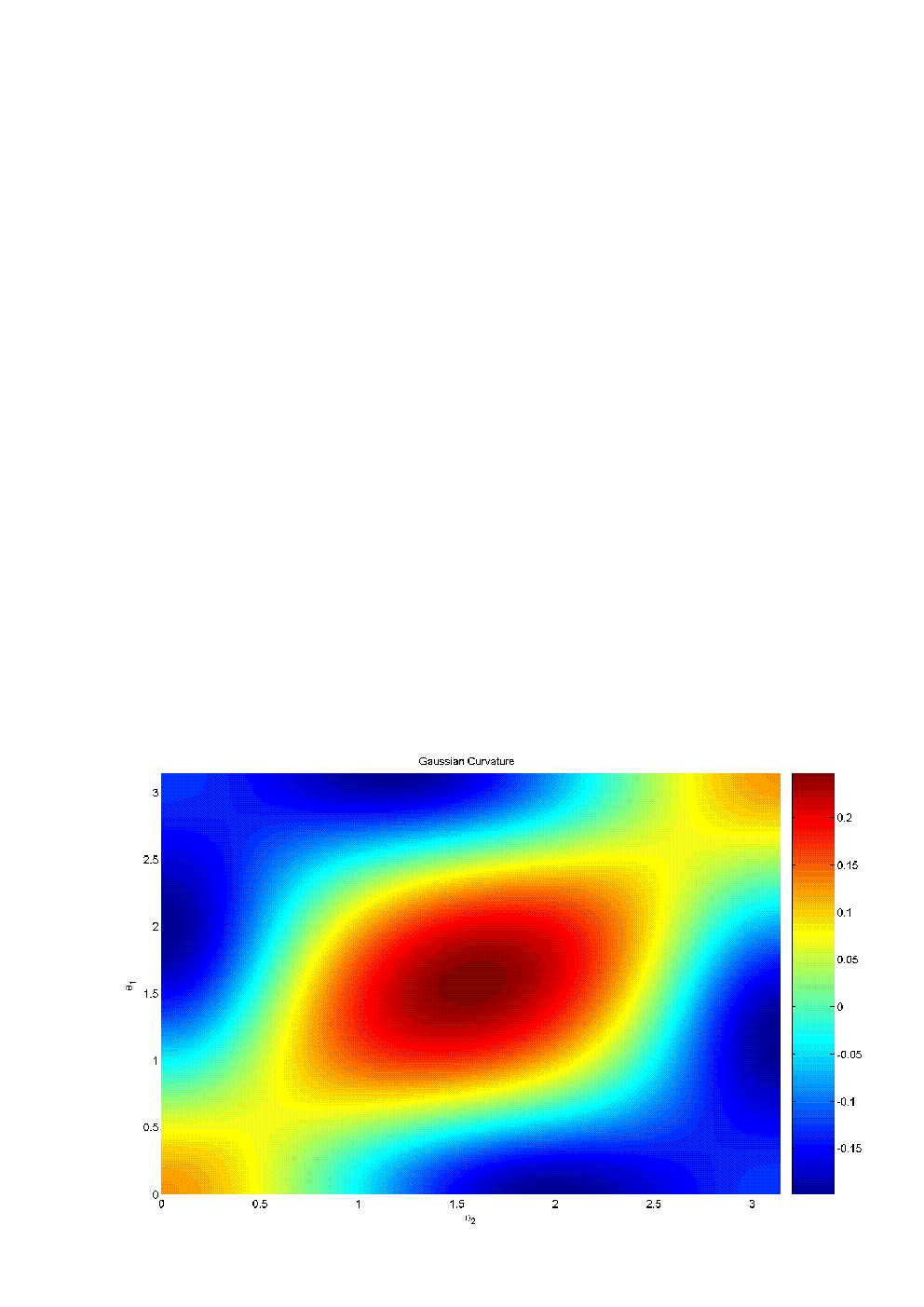
Figure 4: The Gaussian curvature on the surface of controls induced by the dissipation metric.

Inspection of Fig. 3 suggest that pretty good strokes are those that enclose only one sign of the curvature $\mathcal{F}$. The actual optimal stroke can only be found numerically. It is plotted in figure 3. The efficiency for this stroke is about the same as the efficiency of the Purcell’s swimmer for rectangular strokes of [3], but less than the optimally efficient strokes found in [16].

Cox theory does not allow the arms to get too close. How close they are allowed to get depends on the slenderness $\kappa$. The smallest angle allowed $\delta\theta$ must be such that $(2\delta\theta)\log\kappa\gg 1$. As the optimal stroke gets quite close to the boundary, with $\delta\theta\sim 0.1\ radian$ it can be taken seriously only for sufficiently slender bodies with $\log\kappa\gg 5$, which is huge. The optimal stroke is therefore more of mathematical than physical interest. One can use a refine slender body approximation by taking high order terms in Cox’s expansion for the force. This will leave the structure without changes, but will made Eq. 2.6 and Eq. 2.14 much more complicated.

From a mathematical point of view it is actually quite remarkable that a minimizer exists. By this we mean that the optimal stroke does not hit the boundary of shape space $|\xi_{j}|=1$ where Cox theory is squeezed out of existence. This can be seen from the following argument. Inspection of Eq. (2.9) and Eq. (2.14) shows that the curvature vanishes linearly near the boundary of shape space (this is most easily seen in the $\theta$ coordinates). Suppose now that the optimal path ran along the boundary. Shifting the path a distance $\varepsilon$ away from the boundary would shorten it linearly in $\varepsilon$ while the change in the flux integral will be only quadratic. This shows that the path that hits the boundary can not be a minimizer.

3 Purcell swimmer

Purcell swimmer can move in either direction in the plane and can also rotate. Since the Euclidean group is not Abelian (rotations and translations do not commute) the notion of “swimming curvature” that proved to be so useful in the Abelian case needs to be modified. As we shall explain, landscape figures can be used to give qualitative geometric understanding of the swimming and in particular can be used to answer Purcell question “What will determine the direction this swimmer will swim?”. However, unlike the Abelian case, the swimming curvature does not give full quantitative information on the swimming and one can not avoid solving a system of differential equations in this case if one is interested in quantitative details.

The location and orientation of the swimmer (in the Lab frame) shall be denoted by the triplet $x^{\alpha}$ where $x^{0}=\phi$ is the orientation of the swimmer, see Fig. 1, and $x^{1,2}$ are cartesian coordinates of the center of the “body” . We use super-indices and Greek letters to designate the response while lower indices and Roman characters designate the controls $|\theta_{j}|<\pi$.

Linear response versus a gauge theory

The common approach to low Reynolds numbers swimming is to write the equations of motion in a fixed, lab frame. We first review this and then describe an alternate approach where the equations of motions are written in a frame that instantaneously coincides with the swimmer.

By general principles of low Reynolds numbers hydrodynamics there is a linear relations between the change in the controls $d\theta$ and the response $dx$

$$\kern-1.00006pt{\raise 3.44444pt\hbox{ -}}\kern-6.00006pt{d}x^{\alpha}={\mathcal{A}}^{\alpha}_{j}\,d\theta_{j}\,,$$ (3.1)

(summation over repeated indices implied.) Note that $j=1,2$ since there are two controls, while $\alpha=0,1,2$ for the three responses.

The response coefficients $\mathcal{A}$ are functions of both the control coordinates $\theta_{k}$ and the location coordinates $x^{\beta}$ of the swimmer in the Lab. However, in a homogeneous medium it is clear that ${\mathcal{A}}^{\alpha}_{j}$ can only be a function of the orientation $x^{0}=\phi$. Moreover, in an isotropic medium it can only dependent on the orientation $\phi$ through

$$\mathcal{A}^{\alpha}_{i}\left({\phi,\theta}\right)=R^{\alpha\beta}(\phi)A^{\beta}_{i}\left({\theta}\right);\quad R^{\alpha\beta}\left(\phi\right)=\left({\begin{array}[]{*{20}c}1&0&0\\ 0&\cos\phi&-\sin\phi\\ 0&\sin\phi&\cos\phi\\ \end{array}}\right)$$ (3.2)

In the Lab frame, the nature of the solution of the differential equations is obscured by the fact that one can not determine $dx$ independently for different points on the stroke (because of the dependence on $\phi=x^{0}$).

The coefficients $A^{\beta}_{i}$ may be viewed as the transport coefficients in a rest frame that instantaneously coincides with the swimmer. They play a key role in the geometric picture that we shall now describe. In the frame of the swimmer one has

$$\kern-1.00006pt{\raise 3.44444pt\hbox{ -}}\kern-6.00006pt{d}y^{\alpha}=A^{\alpha}_{j}\,d\theta_{j}$$ (3.3)

which is an equation that is fully determined by the controls. The price one pays is that the $\kern-1.00006pt{\raise 3.44444pt\hbox{ -}}\kern-6.00006pt{d}y$ coordinates cannot be simply added to calculate the total change in a stroke $\gamma$, since one has to consider the changes in the reference frame as well. In order to do that, $\kern-1.00006pt{\raise 3.44444pt\hbox{ -}}\kern-6.00006pt{d}y$ must be viewed as (infinitesimal) elements of the Euclidean group

$$E(y^{\alpha})=\left(\begin{array}[]{ccc}\cos y^{0}&\sin y^{0}&y^{1}\\ -\sin y^{0}&\cos y^{0}&y^{2}\\ 0&0&1\\ \end{array}\right)$$ (3.4)

The composition of $\kern-1.00006pt{\raise 3.44444pt\hbox{ -}}\kern-6.00006pt{d}y$ along a stroke $\gamma$ is a matrix multiplication

$$E(\gamma)=\prod_{\theta\in\gamma}E\big{(}dy^{\alpha}(\theta)\big{)}$$ (3.5)

The product is, of course, non commutative. We denote generators of translations and rotations by

$$e^{0}=\left(\begin{array}[]{ccc}0&1&0\\ -1&0&0\\ 0&0&0\\ \end{array}\right),\quad e^{1}=\left(\begin{array}[]{ccc}0&0&1\\ 0&0&0\\ 0&0&0\\ \end{array}\right),\quad e^{2}=\left(\begin{array}[]{ccc}0&0&0\\ 0&0&1\\ 0&0&0\\ \end{array}\right)$$ (3.6)

They satisfy the Lie algebra

$$[e^{0},e^{\alpha}]=-\varepsilon^{0\alpha\beta}e^{\beta},\quad[e^{1},e^{2}]=0$$ (3.7)

where $\varepsilon^{\alpha\beta\gamma}$ is the completely anti-symmetric tensor. One can write Eq. (3.3) concisely as a matrix equation

$$\kern-1.00006pt{\raise 3.44444pt\hbox{ -}}\kern-6.00006pt{d}y=A_{j}d\theta_{j},\quad\kern-1.00006pt{\raise 3.44444pt\hbox{ -}}\kern-6.00006pt{d}y=y^{\alpha}e^{\alpha},\quad A_{j}=A_{j}^{\alpha}e^{\alpha}$$ (3.8)

where $\kern-1.00006pt{\raise 3.44444pt\hbox{ -}}\kern-6.00006pt{d}y$ and $A_{j}$ are $3\times 3$ matrices (summation over repeated indices implied).

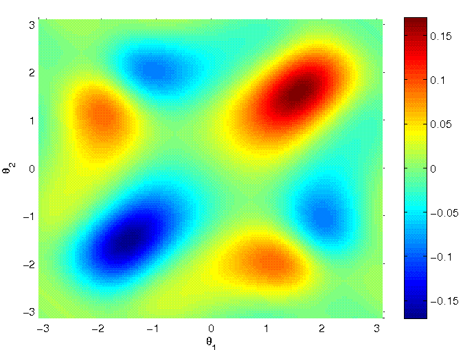
Figure 5: The curvature for rotation for Purcell’s three linked swimmer with $\eta=2$, plotted with the flat measure on $(\theta_{1},\theta_{2})$

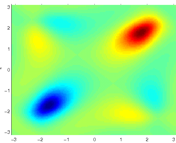
Figure 6: The rotation curvature for Purcell’s three linked swimmer with $\eta=2$ plotted using the measure induced by dissipation

The swimming curvatures

Once the (six) transport coefficients $A^{\alpha}_{j}$ are known, one can, in principle, simply integrate the system of three, first order, non-linear ordinary differential equations, Eq. (3.1). This can normally be done only numerically. Numerical integration is practical and useful, but not directly insightful. We want to describe tools that allow for a qualitative understating swimming in the plane without actually solving any differential equation.

Low Reynolds numbers swimmers perform lots of mutually cancelling maneuvers with a small net effect. The swimming curvature measure only what fails to cancel for infinitesimal strokes. Since reversing a loop reverses the response, it is natural to expect, that $\delta y^{\alpha}$ for a closed (square) loop is proportional to the area form. Integrating Eq. (3.8) around a closed infinitesimal loop gives

$$\delta y=\mathcal{F}d\theta_{1}\wedge d\theta_{2}$$ (3.9)

where

$$\mathcal{F}=\partial_{1}A_{2}-\partial_{2}A_{1}-[A_{1},A_{2}],\quad\mathcal{F}=\mathcal{F}^{\alpha}e^{\alpha},\quad\quad\partial_{j}=\frac{\partial}{\partial\theta_{j}}$$ (3.10)

$\mathcal{F}$ and $\delta y$ are $3\times 3$ matrices. $\mathcal{F}$ has the structure of curvature of a non-abelian gauge field [12]. In coordinates, this reads

$$\mathcal{F}^{\alpha}=\partial_{1}A^{\alpha}_{2}-\partial_{2}A^{\alpha}_{1}+\varepsilon^{0\alpha\beta}\left(A^{0}_{1}A^{\beta}_{2}-A^{0}_{2}A^{\beta}_{1}\right),$$ (3.11)

In the Lab coordinates one has, of course,

$$\delta x^{\alpha}=\mathcal{\tilde{F}}^{\alpha}d\theta_{1}\wedge d\theta_{2},\quad\mathcal{\tilde{F}}^{\alpha}=R^{\alpha\beta}(\phi)\mathcal{F}^{\beta}(\theta),$$ (3.12)

The curvature is Abelian when the commutator vanishes. This is the case in Eq. (2.9) and it is also the case for the rotational curvature. The Abelian curvature gives full information on the swimming of finite stroke by simple application of Stokes formula. This is, unfortunately, not the case in the non-Abelian case. One can not reconstruct the translational motion of a large stroke from the infinitesimal closed strokes $\delta y$ because Stokes theorem only works for commutative coordinates and $\delta y$ are not.

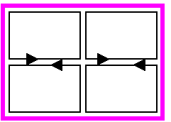
Figure 7: The failure of Stokes theorem in the non-commutative case: The integration on the adjacent segments traversed in opposite senses do not cancel in the non-commutative case.

For Purcell swimmer, $\mathcal{F}$ although explicit, is rather complicated. Since the dissipation metric is complicated too, we give two plots of $\mathcal{F}$: Figs. (5, 8,9) give the curvature relative to the flat measure on $(\theta_{1},\theta_{2})$, and describe how far the swimmer swims for small strokes. In Figs. (6, 10,11) the curvature is plotted relative to the dissipation measure and it displays the energy efficiency of strokes.

The equations of motion

Using Cox theory, in a manner analogous to what was done in for the symmetric swimmer, one can calculate explicitly the force (and torque) on the $a$-th rod in the form

$$F_{a}^{\alpha}=f_{aj}^{\alpha}\dot{\theta}_{j}+f_{a}^{\beta\alpha}\dot{x}^{\beta}$$ (3.13)

where $f_{aj}^{\alpha}$ are explicit and relatively simple functions of the controls (compare with Eq. (2.3)). The swimming equation are then given by

$$\sum_{a}F_{a}^{\alpha}=\left(\sum_{a}f_{aj}^{\alpha}\right)\dot{\theta}_{j}+\left(\sum_{a}f_{a}^{\alpha\beta}\right)\dot{x}^{\beta}=0$$ (3.14)

This reduces the problem of finding the connections $A$ to a problem in linear algebra. Formally

$${A}^{\beta}_{j}=\left(\sum_{a}f_{a}^{\beta\alpha}\right)^{-1}\left(\sum_{a}f_{aj}^{\alpha}\right)$$ (3.15)

where the bracket on the left is interpreted as a $3\times 3$ matrix, with entries $\alpha,\beta$, and the inverse means an inverse in the sense of matrices. Although this is an inverse of only a $3\times 3$ matrix the resulting expressions are not very insightful. We spare the reader this ugliness which is best done using a computer program.

Symmetries

Picking the center point of the body as the reference fiducial point is, in the terminology of Wilczek and Shapere [18] a choice of gauge. This particular choice is nice because it implies symmetries of the connection $A$ [16, 3]. Observe first that the interchange $(\theta_{1},\theta_{2})\rightarrow(-\theta_{2},-\theta_{1})$ corresponds to a rotation of the swimmer by $\pi$. Plugging this in Eq. (3.2) one finds

$$A^{\beta}_{1}(\theta_{1},\theta_{2})=\left\{\begin{array}[]{ll}+A^{\beta}_{2}(-\theta_{2},-\theta_{1}),&\hbox{$\beta=0$;}\\ -A^{\beta}_{2}(-\theta_{2},-\theta_{1}),&\hbox{otherwise.}\\ \end{array}\right.$$ (3.16)

This relates the two half of the square divided by the diagonal $\theta_{1}+\theta_{2}=0$.

A second symmetry comes from the interchange $(\theta_{1},\theta_{2})\rightarrow(\theta_{2},\theta_{1})$ corresponding to the reflection of the swimmer around the central vertical of the middle link. Some reflection shows then that

$$A^{\beta}_{1}(\theta_{1},\theta_{2})=\left\{\begin{array}[]{ll}+A^{\beta}_{2}(\theta_{2},\theta_{1}),&\hbox{$\beta=2$;}\\ -A^{\beta}_{2}(\theta_{2},\theta_{1}),&\hbox{otherwise.}\\ \end{array}\right.$$ (3.17)

This relates the two halves of the square divided by the diagonal $\theta_{1}=\theta_{2}$.

The symmetries can be combined to yield the result that $A^{0}$ and $A^{2}$ are anti-symmetric and $A^{1}$ is symmetric under inversion

$$A^{0}_{j}(\theta)=-A^{0}_{j}(-\theta),\quad A^{1}_{j}(\theta)=A^{1}_{j}(-\theta),\quad A^{2}_{j}(\theta)=-A^{2}_{j}(-\theta)$$ (3.18)

Rotations

The rotational motion of Purcell swimmer, in any finite stroke, is fully captured by the Abelian curvature

$$\mathcal{\mathcal{missing}}{F}^{0}=\mathcal{F}^{0}=\partial_{1}{A}^{0}_{2}-\partial_{2}{A}^{0}_{1}$$ (3.19)

This reflects the fact that rotations in the plane are commutative.

The symmetry of Eq. (3.16) implies

$$(\partial_{2}A^{0}_{1})(\theta_{1},\theta_{2})=(\partial_{1}A^{0}_{2})(-\theta_{2},-\theta_{1})$$ (3.20)

and this says that $\mathcal{F}^{0}$is ani-symmetric under reflection in the diagonal $\theta_{1}+\theta_{2}=0$. Similarly, Eq. (3.21) implies

$$(\partial_{2}A^{0}_{1})(\theta_{1},\theta_{2})=-(\partial_{1}A^{0}_{2})(\theta_{2},\theta_{1}),$$ (3.21)

and this says that $\mathcal{F}^{0}$ is symmetric about the line $\theta_{1}=\theta_{2}$. Fig. (5) is a plot of the curvature and it clearly has the requisite symmetries.

The total curvature associated with the full square of shape space vanishes (by symmetry). For $\eta=2$, one can see in Fig. 5 three positive islands surrounded by three negative lakes. The total curvature associated with the three islands is quite small, about 0.1. This means that Purcell swimmer with $\eta=2$ turns only a small fraction of a circle in any full stroke.

Translation

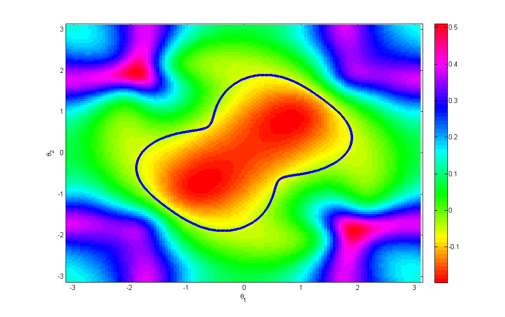
Figure 8: The landscape of the x-curvature for Purcell’s swimmer with $\eta=0.75$ shown with the the Tam and Hosoi optimal distance stroke [16]. The curvature is given relative to the flat measure in $(\theta_{1},\theta_{2})$.

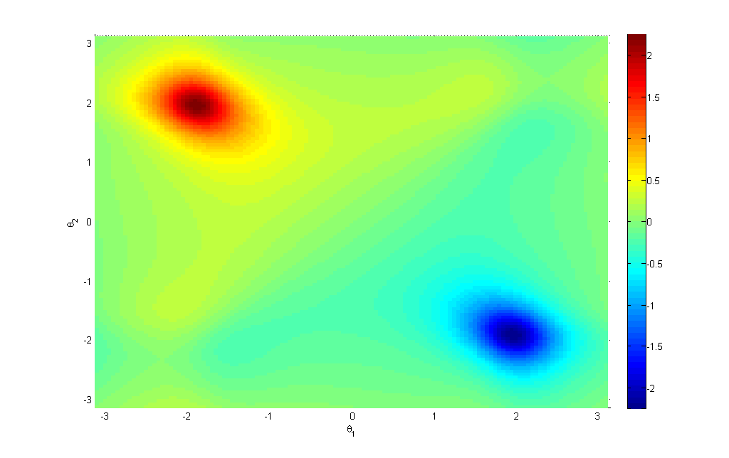
Figure 9: The landscape of the y-curvature for Purcell’s swimmer with $\eta=0.75$. The curvature is given relative to the flat measure in $(\theta_{1},\theta_{2})$.

The curvatures corresponding to the two translations of a swimmer with $\eta=0.75$ are shown in Figs. (8,9,10,11)(here we use $\eta=0.75$ for comparison with [16]). The symmetries of the figures are a consequence of Eqs. (3.16,3.21). Form the first we have

$$(\partial_{2}A^{\beta}_{1})(\theta_{1},\theta_{2})=-(\partial_{1}A^{\beta}_{2})(-\theta_{2},-\theta_{1}),\beta=1,2$$ (3.22)

which implies that $\mathcal{F}^{1,2}$ are symmetric under reflection in the diagonal $\theta_{1}+\theta_{2}=0$. Similarly, from the Eq. (3.21) we have

$$(\partial_{2}A^{\beta}_{1})(\theta_{1},\theta_{2})=\left\{\begin{array}[]{ll}+(\partial_{1}A^{2}_{2})(\theta_{2},\theta_{1}),&\hbox{$\beta=2$;}\\ -(\partial_{1}A^{1}_{2})(\theta_{2},\theta_{1}),&\hbox{$\beta=1$.}\\ \end{array}\right.$$ (3.23)

This says that $\mathcal{F}^{1}$ symmetric and $\mathcal{F}^{2}$ anti-symmetric under reflection in the diagonal $\theta_{1}=\theta_{2}$.

The curvatures for the translations is non-Abelian and can not be used to calculate the swimming distances for finite strokes because the Stokes theorem fails.

4 Qualitative analysis of swimming

When is a stroke small?

The landscape figures for the translational curvatures provide precise information on the swimming distance for infinitesimal strokes. They are then also useful to characterize small strokes. The question is how small is small? For a stroke of size $\varepsilon$, the controls are of size $\delta\theta=O(\varepsilon)$ and the swimming distance measures by the curvature is $O(\mathcal{F}\varepsilon^{2})$. The error in this has terms of the form $O(A\mathcal{F}\varepsilon^{3})$. This suggest that the relative error in the swimming distance as measured a finite stroke is of the order $O(A\varepsilon)$. Hence, a stroke is small provided $|A\varepsilon|\ll 1$. Clearly, a Purcell swimmer swims substantially less than an arm length as the arm moves. This says that $|A|\ll 1$ and so strokes of the order of a radian can be viewed as small strokes.

A radian is the scale of the structures in the landscape of the figures of the curvature. This means that the landscape carries qualitative information about the swimming of moderate strokes.

x versus y

The x-curvature is symmetric under inversion

$$\mathcal{F}^{1}(\theta)=\mathcal{F}^{1}(-\theta)$$ (4.1)

Since both $A^{0}$ and $A^{2}$ are antisymmetric under inversion, one sees that the non-Abelian part of the x-curvature is of order $O(\theta^{2})$ near the origin. The x-translational curvature, which is non-zero near the origin, is almost Abelian for small strokes.

The y-curvature, in contrast, is anti-symmetric under inversion

$$\mathcal{F}^{1}2(\theta)=-\mathcal{F}^{2}(-\theta)$$ (4.2)

and so vanishes linearly at the origin. The non-Abelian part is also anti-symmetric under inversion, and it too vanishes linearly. The y-curvature is therefore not approximately Abelian for small strokes, but it is small.

Which way does a swimmer swim?

The swimming direction can be easily determined for those strokes that live in a region where the translational curvature has a fixed sign. This answers Purcell’s question for many strokes. Strokes the enclose both signs of the curvature are subtle.

Subtle swimmers

Purcell’s swimmer can reverse its direction of propagation by increasing the stroke amplitude [3]. This can be seen from the landscape diagram, Fig. (8): Small square strokes near the origin sample only slightly negative curvature. As the stroke amplitude increases the square gets larger and begins to sample regions where the curvature has the opposite sign, eventually sampling regions with substantial positive curvature.

Optimal distance strokes

The curvature landscapes are useful when one wants to search for optimal strokes as they provide an initial guess for the stroke. (This initial guess can then be improved by standard optimization numerical methods.)

For example, Tam and Hosi [16] looked for strokes that cover the largest possible distance. For strokes near the origin, a local optimizer is the stroke that bounds the approximate square blue region in Fig. 8 (in this case $\eta=0.75$).

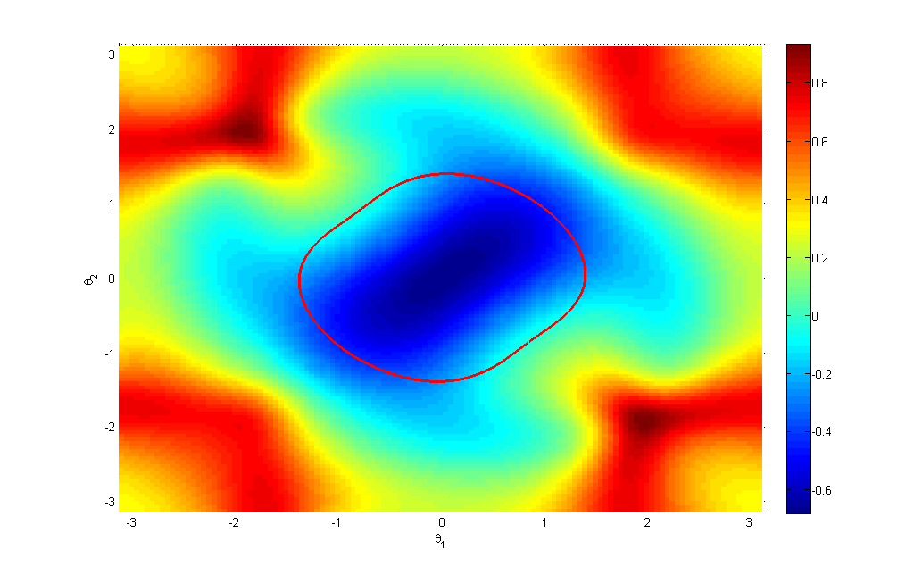
Figure 10: The x-curvature relative to the dissipation metric and the optimal efficient stroke found by Tam and Hosoi [16].

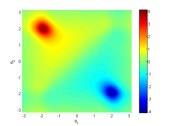
Figure 11: The y-curvature relative to the dissipation metric. Pay attention to the large values in the scale.

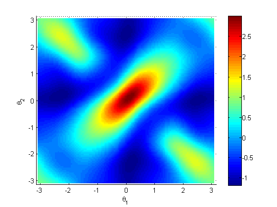
Figure 12: The gaussian curvature induced by the dissipation metric of Purcell’s swimmer

Efficient strokes

The curvature normalized by dissipation, Fig. 10 gives a guide for finding efficient small strokes. Caution must be made, since while the displacement can be approximated from the surface area, the energy dissipation is proportional to the stroke’s length and not the stroke’s area. In regimes where the Gaussian curvature of the dissipation (Fig. 12) is positive - it is possible to have strokes with small length which bounds large area. In the case of Purcell’s swimmer, this suggest two possible regimes: around the origin and the positive curvature island in the upper left (lower right) corner of Fig. 12. The optimizer near the origin is the optimal stroke found in [16], while the optimizer in the upper left corner [14] - although more efficient (pay attention to the values of $\frac{\mathcal{F}^{y}}{\sqrt{\det g(\theta)}}$ in Fig. 11), is of mathematical interest only, since it is near the boundary, where the first order slender body approximation Eq.( 2.1) is relevant only for extremely slender bodies.

Acknowledgment

We thank A. Leshanskey and O. Kenneth for discussions.

References

- [1] J. E. Avron, O. Kenneth , and D. H. Oaknin. Pushmepullyou: an efficient micro-swimmer. New J. Phys., 7(234):8, 2005.
- [2] J. E. Avron and and O. Kenneth O. Gat. Optimal swimming at low reynolds numbers. Phy. Rev. Lett., 93(18):186001, 2004.
- [3] L. E. Becker, S. A. Koehler, and H. A. Stone. On self-propulsion of micromachines at low reynolds number: Purcell’s three-link swimmer. J. of Fluid Mech., 490:15–35, 2003.
- [4] S. Chattopadhyay, R. Moldovan, C. Yeung, and X. L. Wu. Swimming efficiency of bacterium escherichia coli. Proc. Nat. Acc. Sci., 103(13):13712–13717, September 2006.
- [5] R. G. Cox. The motion of long slender bodies in a viscous fluid part 1. general theory. Journal of Fluid Mech., 44(4):791–810, December 1970.
- [6] G. A. de Araujo and J. Koiller. Self-propulsion of n-hinged ’animats’ at low reynolds number. Qual. Theory Dyn. Sys., 4(58):139–167, 2004.
- [7] R. Dreyfus, J. Baudry, M. Roper, M. Fermigier, H. Stone, and J. Bibette. Microscopic artificial swimmer. Nature, 437:862–865, 2005.
- [8] R. Gilad, A. Porat, and S. Trachtenberg. Motility modes of spiroplasma melliferum bc3: ahelical, well-less bacterium deriven by linear motor. Molecular Micribiology, 47(3):657–669, February 2003.
- [9] R. Golestanian and A. Najafi. Simple swimmer at low reynolds number: Three linked spheres. Phys. Rev. E, 69:062901–062905, 2004.
- [10] and H. Brenner J. Happel. Low Reynolds number hydrodynamics. Kluwer, second edition, 1963.
- [11] A. M. Leshansky, O. Kenneth, O. Gat, and J.E. Avron. A frictionless microswimmer. New J. Phys., 2007.
- [12] M. Nakahara. Geometry, Topology and Physics. IOP, second edition.
- [13] E. M. Purcell. Life at low reynolds number. American Journal of Physics, 45(1):3–11, January 1977.
- [14] O. Raz and J. E. Avron. A comment on ”optimal stroke patterns for purcell’s three-linked swimmer”. Phys. Rev. Lett., In press.
- [15] M. Spivak. A Comprehensive Introdaction to Differential Geometry, volume 2. Publish or Perish Inc., 1979.
- [16] D. Tam and A. E. Hosoi. Optimal stroke patterns for purcell’s three-linked swimmer. Phys. Rev. Lett., 98:4, February 2007.
- [17] H. Wada and R. R. Netz. Model for self-propulsive helical filaments: Kink-pair propagation. Phys. Rev. Lett., 99(10):108102, 2007.
- [18] F. Wilczek and A. Shapere. Geometry of self-propulsion at low reynolds number. J. of Fluid Mech., 198:557–585, 1989.