THE ANGULAR CLUSTERING OF DISTANT GALAXY CLUSTERS

Abstract

We discuss the angular clustering of galaxy clusters at $z>1$ selected within 50 deg² from the Spitzer Wide-Infrared Extragalactic survey. We employ a simple color selection to identify high redshift galaxies with no dependence on galaxy rest–frame optical color using Spitzer IRAC 3.6 and 4.5 µm photometry. The majority ($>$90%) of galaxies with $z>1.3$ are identified with $(\hbox{$[3.6]$}-\hbox{$[4.5]$})_{\mathrm{AB}}>-0.1$ mag. We identify candidate galaxy clusters at $z>1$ by selecting overdensities of $\geq$26–28 objects with $\hbox{$[3.6]$}-\hbox{$[4.5]$}>-0.1$ mag within radii of 1.4 arcminutes, which corresponds to $r<0.5\;h^{-1}$ Mpc at $z=1.5$. These candidate galaxy clusters show strong angular clustering, with an angular correlation function represented by $w(\theta)=(3.1\pm 0.5)(\theta/1\arcmin)^{-1.1\pm 0.1}$ over scales of 2–100 arcminutes. Assuming the redshift distribution of these galaxy clusters follows a fiducial model, these galaxy clusters have a spatial–clustering scale length $r_{0}=22.4\pm 3.6\,h^{-1}$ Mpc, and a comoving number density $n=1.2\pm 0.1\times 10^{-6}h^{3}$ Mpc^-3. The correlation scale length and number density of these objects are comparable to those of rich galaxy clusters at low redshift. The number density of these high–redshift clusters correspond to dark–matter halos larger than $3-5\times 10^{13}$ $h^{-1}$ $\mathcal{M}_{\odot}$ at $z=1.5$. Assuming the dark halos hosting these high–redshift clusters grow following $\Lambda$CDM models, these clusters will reside in halos larger than $1-2\times 10^{14}$ $h^{-1}$ $\mathcal{M}_{\odot}$ at $z=0.2$, comparable to rich galaxy clusters.

1. Introduction

Clusters of galaxies provide important samples for studying structure evolution and cosmology. They trace large dark mass halos, which collapsed early in the history of the Universe, and thus they probe the structure of overdensities in the underlying dark–matter distribution (Springel et al., 2005). This is evident in the strong spatial clustering inferred for galaxy cluster samples, which find typical spatial correlation function scale lengths of $r_{0}\sim 20-30$ $h^{-1}$ Mpc for optically and X-ray selected galaxy clusters in the local and distant Universe (e.g., Bahcall, 1988; Abadi et al., 1998; Lee & Park, 1999; Collins et al., 2000; Gonzalez et al., 2002; Bahcall et al., 2003; Brodwin et al., 2007). Furthermore, the expected number density of galaxy clusters is sensitive to the cosmic matter density, $\Omega_{m}$ (e.g., Kitayama & Suto, 1996; Wang & Steinhardt, 1998). Currently, both the measured correlation function scale lengths and number densities of galaxy clusters support theoretical predictions for standard cold dark–matter models, which include a cosmological constant (e.g., Bahcall et al., 2003). Therefore, because galaxy clusters correspond to large matter overdensities, their number density evolution with redshift provides constraints on cosmological parameters, and these constraints should be amplified at higher redshifts (e.g., when the Universe was matter dominated; see Haiman, Mohr, & Holder, 2001).

Galaxy clusters also provide laboratories for studying galaxy formation. Galaxy clusters contain a population of galaxies that evolved early in the history of the Universe. Locally, clusters contain a high fraction of early–type, elliptical and lenticular galaxies, which contain little ongoing star formation (e.g., Dressler, 1980), and the fraction of early–type galaxies in clusters appears to evolve strongly with redshift (e.g., Lubin et al., 1998; van Dokkum et al., 2000). Studies of the stellar populations of the early–type cluster galaxies at $z\lesssim 1$ show they have evolved nearly passively from $z_{f}\sim 2-3$ (e.g., Postman et al., 1998; Stanford, Eisenhardt, & Dickinson, 1998; van Dokkum & Franx, 2001; van Dokkum & van der Marel, 2007). Studying clusters at $z\gtrsim 1$ provides constraints on the formation of the massive, early–type galaxies within them (e.g., Eisenhardt et al., 2007).

Identifying galaxy clusters at $z\gtrsim 1$ presents some significant technical and physical challenges. Deep X-ray surveys identify distant clusters at cosmologically significant redshifts, because the X-ray luminosity scales with the mass of the cluster and it is relatively unaffected by projection effects (e.g., Rosati et al., 2004). Spectroscopic observations of galaxies associated with faint, diffuse X–ray emission have identified clusters at redshifts (to date) of $z=1.41$–1.45 (Mullis et al., 2005; Stanford et al., 2006). However, the X-ray surface brightness declines strongly with redshift ($\propto[1+z]^{4}$), biasing against high–redshift clusters with relatively diffuse emission. Furthermore, X–ray emission from hot ($T\sim 10^{6}-10^{7}$ K) gas in the inter-cluster medium generally requires a dynamically relaxed, virialized, massive system. This may not be the case at high redshifts during the hierarchical assembly of the dark matter halos where cluster progenitors will be less massive and likely disrupted (e.g., Rosati et al., 2002). Searches for high–redshift clusters have also targeted fields around distant radio galaxies as “signposts” of large dark–matter overdensities (Kurk et al., 2000; Venemans et al., 2002, 2007; Stern et al., 2003; Miley et al., 2004; Croft et al., 2005; Kajisawa et al., 2006; Kodama et al., 2007). While these have been successful, these studies require the presence of a massive, central galaxy, which may not be an intrinsic, ubiquitous feature to the high–redshift progenitors of all clusters.

Using ground–based optical and near–IR, or Spitzer near–IR imaging, recent searches for clusters rely on identifying overdensities of galaxies with red optical to near–IR colors (e.g., Gladders & Yee, 2005; Gladders et al., 2007; Kajisawa et al., 2006; Wilson et al., 2006; Kodama et al., 2007), which correspond to galaxies with evolved stellar populations with strong Balmer/4000 Å breaks at $z\gtrsim 1$. While these surveys have had success, the cluster selection based on red galaxy colors may be biased away from potential clusters dominated by galaxies with relatively blue colors. For example, any study of the evolution of galaxies in these clusters are subject to a form of “progenitor” bias in that one identifies only those clusters dominated by red, presumably early-type galaxies (see, e.g., van Dokkum & Franx, 2001). Because these red, early-type galaxies that dominate galaxy clusters at present formed their stellar populations at $z\gtrsim 1$ (see references above), one expects that their progenitors should show increasing indications of ongoing star formation at these epochs. Furthermore, there is evidence that the relative fraction of galaxies with blue colors in overdense environments increases with redshift (Gerke et al., 2007), with luminous blue galaxies at $z\sim 1$ preferentially residing in regions of greater–than–average overdensity (Cooper et al., 2007). For example, Elbaz et al. (2007) found that the average star formation rates of galaxies at $z\sim 1$ in dense environments are higher than those of other co–eval galaxies in less dense environments. Certainly by $z\gtrsim 1.5$ there exist strong overdensities of blue, rest-frame UV–selected galaxies (Steidel et al., 1998; Adelberger et al., 2005; Steidel et al., 2005), and such systems would presumably be missed by traditional searches for red galaxies. For example, Brodwin et al. (2006, see also Eisenhardt et al. 2007) and van Breukelen et al. (2006) identify high–redshift cluster candidates as overdensities of galaxies with similar photometric redshifts, and these efforts have yielded some of the highest redshift clusters yet identified at $z=1.41$ (Stanford et al., 2005) and $z=1.45$ (van Breukelen et al., 2007).

Here, we use a simple color selection to identify galaxies at $z\gtrsim 1$ based solely on red colors between IRAC channels 1 and 2 (3.6 and 4.5 µm). This selection has little dependence on galaxy rest-frame optical color, it is sensitive to red and blue galaxies nearly equally. This technique utilizes the fact that nearly all plausible stellar populations show a peak in their $f_{\nu}$ emission at 1.6 µm  accompanied by a steady decline on the Rayleigh–Jeans tail of the stellar emission (see Simpson & Eisenhardt 1999; Sawicki 2002; van Dokkum et al. 2007). All composite stellar populations in galaxies at $z\lesssim 1$ have blue IRAC $\hbox{$[3.6]$}-\hbox{$[4.5]$}$ colors because these bands sit on the Rayleigh–Jeans tail of the stellar emission, while at $z\gtrsim 1$ galaxies appear redder in IRAC $\hbox{$[3.6]$}-\hbox{$[4.5]$}$ color as these bands probe the peak of the stellar emission. A similar technique has been applied by Takagi et al. (2007) to identify galaxies at $z\gtrsim 0.5$ using $[2.2]-[3.5]>0.1$ mag colors from the AKARI satellite, analogous to the technique used here. We identify candidates for high–redshift, $z\gtrsim 1$, galaxy clusters from overdensities of those galaxies with IRAC $\hbox{$[3.6]$}-\hbox{$[4.5]$}>-0.1$ mag colors. Strictly speaking, these galaxy overdensities are candidates for galaxy clusters, and must be confirmed by spectroscopy. Nevertheless, we show that even these candidates for galaxy clusters provide a useful sample for studying galaxy evolution and cosmology at high redshifts.

A strong motivation for this study is the proposed Spitzer mission in the post–cryogenic era (starting ca. 2009 April), which may provide a tremendous amount of observing time ($>$$10^{4}$ hrs) with only IRAC channels 1 and 2. This study demonstrates one possible science driver for a warm Spitzer mission (see also van Dokkum et al., 2007). The outline for the rest of this paper is as follows. In § 2 we describe the datasets used for the study. In § 3 we describe the method to identify distant galaxy clusters from Spitzer/IRAC data. In § 4 we compute the angular clustering of the distant galaxy clusters. In § 5 we discuss the redshift selection function and number density of these clusters, we derive their spatial clustering correlation length from the angular correlation function, and we describe the evolution of these galaxy clusters. Throughout this work we quote optical and near–IR magnitudes on the AB system where $m_{\mathrm{AB}}=23.9-2.5\log(f_{\nu}/1\;\hbox{$\mu$Jy})$. We denote magnitudes measured from the data with Spitzer/IRAC in the four channels [3.6], [4.5], [5.8], [8.0], respectively. Throughout, we use a cosmology with $\Omega_{m}=0.3$, $\Lambda=0.7$, and $H_{0}=100\,h$ km s^-1 Mpc^-1. To compare with other results, we assume a Hubble parameter $h=1.0$.

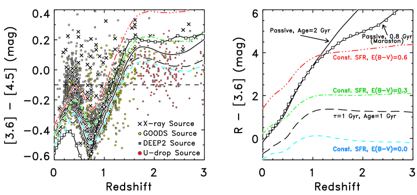
Figure 1.— Galaxy colors as a function of redshift. The left panel shows the $\hbox{$[3.6]$}-\hbox{$[4.5]$}$ color as a function of redshift, and the right panel shows the $R-\hbox{$[3.6]$}$ color as function of redshift. The data points for $\sim$10⁴ objects are shown only in the left panel for clarity. The pentagons and squares denote sources from GOODS and DEEP2 with high–quality spectroscopic redshifts. Crosses show those sources detected in X-ray data. Red circles show blue, star–forming galaxies with spectroscopic redshifts $1.5<z<3$ from Shapley et al. (2005) and Reddy et al. (2006). The horizontal dashed line shows the $\hbox{$[3.6]$}-\hbox{$[4.5]$}>-0.1$ mag color criterion. The curves show the colors expected from various integrated stellar population models, labeled in the right panel. The white boxes connected by the solid line shows the colors expected for a passively evolving stellar population with $t=0.8$ Gyr from Maraston (2005). The other curves assume the Bruzual & Charlot (2003) model. The solid line corresponds to a passively evolving stellar population with an age $=2$ Gyr. The long–dashed line corresponds to a stellar population with an exponentially declining star–formation rate, $\exp(-t/\tau)$ with $\tau=t=1$ Gyr. The short–dashed, dot–dashed, and triple-dot–dashed lines correspond to a stellar population with constant star–formation and dust extinction of $E(B-V)$=0.0, 0.3, and 0.6, respectively, assuming the Calzetti et al. (2000) extinction law.

2. The Datasets

To demonstrate the utility of using IRAC colors to identify galaxies with $z\gtrsim 1$, we use two datasets with ample spectroscopic redshifts and deep IRAC imaging. These are the southern Great Observatories Origins Deep Survey (GOODS–S; Dickinson et al. 2003; Giavalisco et al. 2004) and the All-wavelength Extended Groth strip International Survey (AEGIS; Davis et al. 2007). Although other datasets with comparable IRAC data and spectroscopic data exist, they would add little to the discussion here. However, we do include the samples of UV–bright, star–forming galaxies (so–called “U–dropouts”) with $1.5<z<3$ from Shapley et al. (2005) and Reddy et al. (2006) to augment the galaxies with IRAC data and spectroscopy at higher redshifts. For the bulk of the study here, we use available catalogs from the Spitzer Wide-Infrared Extragalactic (SWIRE) survey, which cover the largest area with deep Spitzer data.

2.1. The GOODS dataset

GOODS–S includes deep Spitzer/IRAC imaging to a depth of 25 hr. per band at 3.6, 4.5, 5.8, and 8.0 µm over a $10\arcmin\times 15\arcmin$ in the southern Chandra Deep Field. These data reach limiting $5\sigma$ flux sensitivities for point sources of 0.11 and 0.21 $\mu$Jy at 3.6 and 4.5 µm, respectively (M. Dickinson et al. 2007, in preparation). The GOODS–S field has extensive spectroscopy. Here we use the published redshifts of Le Fèvre et al. (2004), Szokoly et al. (2004), Mignoli et al. (2005), and Vanzella et al. (2005, 2006), which provide 1624 redshifts for GOODS IRAC sources. For this field we also make use of the X-ray catalog from deep (1 Msec) Chandra data (Alexander et al. 2003), which provides X-ray counterparts to 133 of the IRAC sources with spectroscopic redshifts.

2.2. The AEGIS dataset

The AEGIS program includes deep Spitzer/IRAC imaging to a depth of 3 hr. per band at 3.6, 4.5, 5.8, and 8.0 µm over a $15\arcmin\times 2^{\circ}$ field in the Groth Strip (Davis et al. 2007). These data reach $5\sigma$ depths of 0.9 $\mu$Jy at 3.6 and 4.5 µm (Barmby et al., 2007). This field covers the DEEP2 spectroscopic survey using Keck/DEIMOS, and provides redshifts for $>$8000 IRAC sources. Spectroscopic targets for DEEP2 extend to sources with $R<24.1$ mag, although the $R$–band imaging identifies sources to a limiting magnitude of $R=24.7$ mag ($5\sigma$; see, Davis et al. 2007). We also use the X-ray catalog from 200 ksec data in this field (Nandra et al., 2005), which provides X-ray counterparts to 32 IRAC sources with spectroscopic redshifts.

2.3. The SWIRE dataset

For the work here, we use data from the SWIRE legacy survey (Lonsdale et al., 2003). SWIRE covers six fields with Spitzer/IRAC to 120 s depth, reaching estimated $5\sigma$ flux limits of 3.7 and 5.4 $\mu$Jy at 3.6 and 4.5 µm, respectively. The SWIRE fields cover roughly 50 deg² in total, including 7.8 deg² in the southern Chandra Deep Field (CDF–S), 11.0 deg² in the Lockman Hole, 9.2, 4.8, and 6.9 deg² in the N1, N2, and S1 fields of the European Large-area ISO Survey (ELAIS) fields, and 9.2 deg² in the XMM Large–Scale Survey (XMM-LSS), respectively. For the study here, we used the SWIRE IRAC data from the publicly available third data release (DR3), as described in Surace et al. (2005).

3. The High Redshift Galaxy Cluster Sample

3.1. IRAC Color Selection of High–Redshift Galaxies

Based on our understanding of the emission of composite stellar populations, galaxies at high redshift should have relative uniformity in their IRAC $\hbox{$[3.6]$}-\hbox{$[4.5]$}$ colors. Figure 1 shows the expected behavior of the $\hbox{$[3.6]$}-\hbox{$[4.5]$}$ color as a function of redshift for various stellar population models. The curves in the figure correspond to a wide range of composite model stellar populations, using both the Bruzual & Charlot (2003) models (including dust extinction from Calzetti et al. 2000), and the Maraston (2005) models. The diversity in the models is reflected in the variation in their $R-\hbox{$[3.6]$}$ colors, shown in the right panel of figure 1. These models include purely passive, old stellar populations formed in an instantaneous burst, models with exponentially declining star formation rates, and models with constant star–formation rates and various dust attenuation. Even thought the models are diverse, they span a tight locus in $\hbox{$[3.6]$}-\hbox{$[4.5]$}$ color, showing a characteristic “S” shape with a local maximum at $z\sim 0.3$, a local minimum at $z\sim 0.7$, and a rise to red colors for $z\gtrsim 1$. For $z\lesssim 1$ the composite stellar population models have relatively blue $\hbox{$[3.6]$}-\hbox{$[4.5]$}$ colors as these are dominated from stellar emission at $\lambda>2$ µm, which corresponds to the Rayleigh–Jeans tail of stellar spectra. The rise at $z\gtrsim 1$ results as the IRAC $[3.6]$ and $[4.5]$ bands shift to wavelengths $\lesssim 2$ µm, where they probe the peak in the stellar emission (in $f_{\nu}$ units) near 1.6 µm (e.g., Sawicki 2002). At yet higher redshifts, IRAC probes $\lambda<1$ µm, where composite stellar populations have relatively red $\hbox{$[3.6]$}-\hbox{$[4.5]$}$ colors.

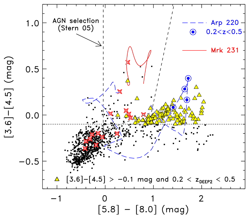
Figure 2.— IRAC $\hbox{$[5.8]$}-\hbox{$[8.0]$}$ versus $\hbox{$[3.6]$}-\hbox{$[4.5]$}$ colors for objects in the AEGIS field with high–quality spectroscopic redshifts and high–S/N IRAC photometry. Yellow triangles denote those objects with $0.2<z_{\mathrm{DEEP2}}<0.5$ and $\hbox{$[3.6]$}-\hbox{$[4.5]$}>-0.1$ mag (indicated by the dotted line). Such objects do not generally populate the mid–IR color selection for obscured AGN proposed by Stern et al. (2005), bounded by the dashed region. The colored curves show the expected colors as a function of redshift for the IR–luminous galaxies Arp 220, dominated by star–formation (blue, dashed line), and Mrk 231, which hosts an obscured AGN (red solid line). Red stars show X-ray–detected sources. Sources denoted by the yellow triangles have red IRAC colors consistent with warm dust associated with star-formation in objects with $0.2<z<0.5$ such as Arp 220 (the redshifts $0.2<z<0.5$ for Arp 220 are indicated by large blue circles).

.

Existing IRAC data show that high–redshift galaxies generally have $\hbox{$[3.6]$}-\hbox{$[4.5]$}$ colors within expectations from the composite stellar population models. Figure 1 shows the IRAC colors for galaxies with high spectroscopic quality in the GOODS–S and AEGIS fields, and the blue, star–forming galaxies at higher redshift from Shapley et al. (2005) and Reddy et al. (2006) (see § 2). The bulk of the data mirror the characteristic “S” shape expected from the models, although there are noticeable outliers. Many sources with putative AGN based on the X-ray data have red $\hbox{$[3.6]$}-\hbox{$[4.5]$}$ colors for all redshifts. These objects presumably have a contribution to their emission at $1-3$ µm arising from dust heated by an AGN. There is also a subset of galaxies with $0.2<z<0.5$ with $\hbox{$[3.6]$}-\hbox{$[4.5]$}$ colors redder than predicted by any of the composite stellar population models. These colors do not arise from differences in the modeling the evolution of post–main sequence stars. Figure 1 shows the expected colors from a stellar population with enhanced rest–frame near-IR emission from thermally pulsating asymptotic giant branch stars (Maraston, 2005). Although the figure shows this model for only one possible age (0.8 Gyr, near the peak of the contribution of post–main–sequence stars to the bolometric emission; Maraston 2005), no other possible age and star-formation history for this model matches the points with $\hbox{$[3.6]$}-\hbox{$[4.5]$}>-0.1$ mag at $0.2<z<0.5$.

Interestingly, the objects with $0.2<z<0.5$ and $\hbox{$[3.6]$}-\hbox{$[4.5]$}>-0.1$ mag do not generally have colors consistent with AGN. Figure 2 shows the IRAC $\hbox{$[5.8]$}-\hbox{$[8.0]$}$ versus $\hbox{$[3.6]$}-\hbox{$[4.5]$}$ colors for objects in the DEEP2 field with high–S/N IRAC photometry and high–quality spectroscopic redshifts. The objects at $0.2<z<0.5$ with $\hbox{$[3.6]$}-\hbox{$[4.5]$}>-0.1$ mag have $\hbox{$[5.8]$}-\hbox{$[8.0]$}$ colors redder than expected for obscured AGN (Stern et al., 2005). Instead, these objects have IRAC colors consistent with IR–luminous star-forming galaxies, such as Arp 220. In such objects the red $\hbox{$[3.6]$}-\hbox{$[4.5]$}$ colors result from warm dust heated by star–formation at rest–frame $\lambda>2$ µm (Imanishi et al., 2006). The red $\hbox{$[5.8]$}-\hbox{$[8.0]$}$ colors result at $z>0.2$ as the strong mid–IR emission features at $\lambda>6$ µm shift out of the $[5.8]$ bandpass (but remain in the $[8.0]$ bandpass until $z\simeq 0.5$). Therefore, the population of galaxies with $0.2<z<0.5$ with $\hbox{$[3.6]$}-\hbox{$[4.5]$}>-0.1$ mag are star-forming galaxies with a strong contribution of warm dust emission at rest–frame $\lambda>3$ µm over what is expected from composite stellar populations.

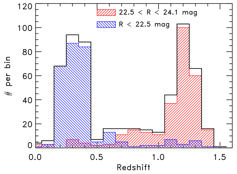
Figure 3.— The redshift distribution of sources with $\hbox{$[3.6]$}-\hbox{$[4.5]$}>-0.1$ mag for sources with high quality redshifts from the DEEP2 spectroscopic survey. The solid line shows the distribution of galaxies satisfying this IRAC color cut. The blue–shaded and red–shaded histograms show the redshift distribution of those galaxies with $R<22.5$ mag and $22.5\leq R<24.1$ mag, respectively. The appreciable decline in the number of sources with redshift at $z\gtrsim 1.2$ results from the spectroscopic incompleteness of the DEEP2 survey.

Based on figure 1 the $\hbox{$[3.6]$}-\hbox{$[4.5]$}>-0.1$ mag selection identifies galaxies with $0.2<z<0.5$ and $z>1$. Including an apparent magnitude criterion further differentiates these galaxies. Figure 3 shows the redshift distribution of the $\hbox{$[3.6]$}-\hbox{$[4.5]$}>-0.1$ mag galaxies with $R\leq 22.5$ mag and $22.5<R<24.1$ mag for galaxies with high–quality DEEP2 spectroscopic redshifts (where $R=24.1$ mag is the limiting magnitude for the DEEP2 spectroscopy). The objects from DEEP2 in this figure include only those with IRAC 3.6 and 4.5 µm flux densities above the SWIRE IRAC detection limit. Thus, the redshift distribution is applicable to the SWIRE data used below. The vast majority of sources with $R<22.5$ mag also have $0.2<z<0.5$, whereas most galaxies with $R>22.5$ mag have $z>1.1$. The appreciable decline in the number of sources with redshift at $z\gtrsim 1.2$ results from the spectroscopic incompleteness of the DEEP2 survey. Based on figure 1, we expect that the redshift distribution of galaxies with $\hbox{$[3.6]$}-\hbox{$[4.5]$}>-0.1$ mag and $R>22.5$ mag will certainly extend to redshifts greater than 1.4.

Even in the absence of deep optical imaging, the selection of $\hbox{$[3.6]$}-\hbox{$[4.5]$}>-0.1$ mag sources preferentially identifies high–redshift galaxies. Galaxies with $\hbox{$[3.6]$}-\hbox{$[4.5]$}>-0.1$ mag and $R<22.5$ mag constitute only $\simeq$20% of all objects with DEEP2 spectroscopic redshifts and IRAC 3.6 and 4.5 µm flux densities brighter than the SWIRE flux limit. Furthermore, among all galaxies in the AEGIS field with $\hbox{$[3.6]$}-\hbox{$[4.5]$}>-0.1$ mag (with or without spectroscopic redshifts) 80% have $R>22.5$ mag, implying the majority of these have $z\gtrsim 1$. Therefore, galaxies with $\hbox{$[3.6]$}-\hbox{$[4.5]$}>-0.1$ mag account for the majority of galaxies with $z\gtrsim 1$. Figure 4 shows the fraction of galaxies with $\hbox{$[3.6]$}-\hbox{$[4.5]$}>-0.1$ as a function of redshift from the high–quality spectroscopic redshifts in the AEGIS field. More than 50% (90%) of the galaxies with $z>1.1$ (1.3) satisfy the IRAC color–selection criteria, $\hbox{$[3.6]$}-\hbox{$[4.5]$}>-0.1$ mag, and this increases to 100% for AEGIS galaxies with $z>1.4$. Moreover, $\simeq 90$% of the galaxies at $1.5<z<3$ from Shapley et al. (2005) and Reddy et al. (2006) satisfy $\hbox{$[3.6]$}-\hbox{$[4.5]$}>-0.1$ mag (the “U–dropouts”, see figure 1). The IRAC color selection is highly efficient at identifying high redshift galaxies.

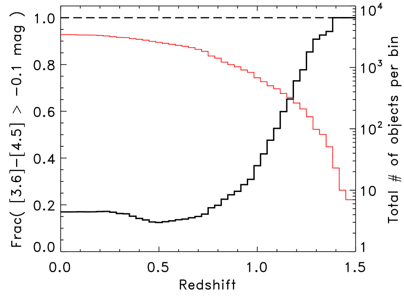
Figure 4.— The fraction of sources with $\hbox{$[3.6]$}-\hbox{$[4.5]$}>-0.1$ mag as a function of redshift from the DEEP2 spectroscopic survey. The thin, red line shows the total number of all objects in the DEEP2 spectroscopic catalog. The thick, black line shows the fraction of those sources with $\hbox{$[3.6]$}-\hbox{$[4.5]$}>-0.1$ mag. More than 90% of the sources at $z>1.3$ have $\hbox{$[3.6]$}-\hbox{$[4.5]$}>-0.1$ mag.

3.2. Identification of High Redshift Clusters

We identify candidate galaxy clusters as overdensities of galaxies satisfying the color selection $\hbox{$[3.6]$}-\hbox{$[4.5]$}>-0.1$ mag in the SWIRE data. We take all objects in the SWIRE IRAC catalogs for each of the six fields (see § 2.3) with $\hbox{$[3.6]$}-\hbox{$[4.5]$}>-0.1$ mag, and S/N$(3.6\micron)>10$ and S/N$(4.5\micron)>10$. The S/N limit ensures that only well-detected objects enter the sample. In practice, this limits the analysis to objects with $f_{\nu}(3.6)>7-10$ $\mu$Jy. Using a pure flux-density limit does not affect the results here, but increases the possibility that the sample will contain spurious sources with low significance or uncertain IRAC colors. The goal here is to identify a robust set of candidate galaxy clusters.

To define candidate galaxy clusters, we count the number of galaxies within a given radius on the sky. For each galaxy in the sample with $\hbox{$[3.6]$}-\hbox{$[4.5]$}>-0.1$ mag, we count the number of other galaxies satisfying this color criterion within a radius of $1\farcm 4$. For $1<z<2.5$ (the approximate range the expected redshift distribution given our selection, see § 5.1) $1\farcm 4$ corresponds to an angular diameter distance of $\approx$0.5 $h^{-1}$Mpc (for $\Omega_{m}=0.3$ and $\Lambda=0.7$). This size is smaller than the typical size used to identify galaxy clusters in optical data (e.g., Bahcall et al. 2003), but this size encompasses typical cluster–core sizes. Moreover, the smaller radius used here reduces greatly the number of chance alignments along the line of sight, which scale as $\propto r^{2}$. Experiments using larger radii for this selection require a substantially greater number of sources to exceed the $3\sigma$ threshold (see below), and identify objects with greater angular clustering.

Figure 5 shows the distribution of the number of companions with $\hbox{$[3.6]$}-\hbox{$[4.5]$}>-0.1$ mag within $r<1\farcm 4$ for the Lockman Hole SWIRE field. In this case, the mean number of galaxies with these IRAC colors within $r<1\farcm 4$ is $\langle N\rangle\simeq 15.6$. The distribution is skewed toward objects with an excess number of companions (this is the case for all the other SWIRE fields as well), which indicates the strong clustering of these sources. If the overdensities of objects result from projection effects of unassociated objects along the line of sight, or from other random processes, then the distribution in figure 5 would be more consistent with a Gaussian distribution.

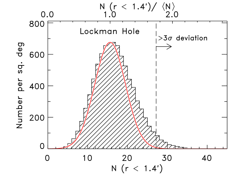
Figure 5.— The distribution of the number of objects with $\hbox{$[3.6]$}-\hbox{$[4.5]$}>-0.1$ mag within $r<1\farcm 4$ for sources in the Lockman Hole field. The mean number of objects is $\langle N(r<1\farcm 4)\rangle=15.6$. The measured distribution is skewed to objects with a high number of companions. The red curve shows a Gaussian fit to the clipped distribution. The vertical dashed line shows three standard deviations of the Gaussian distribution, corresponding to objects with $\geq 27$ companions with $\hbox{$[3.6]$}-\hbox{$[4.5]$}>-0.1$ mag within $r<1\farcm 4$.

We fit a Gaussian to the distribution of the number of objects with $\hbox{$[3.6]$}-\hbox{$[4.5]$}>-0.1$ mag within $r<1\farcm 4$ for each of the SWIRE fields. For each field, we fit a Gaussian to the distribution iteratively clipping at $2\sigma$. This fit is drawn on the distribution in figure 5 for the Lockman Hole, and it matches the left–hand side of the observed distribution very well. We then defined the sample of galaxy cluster candidates to be those objects with more than $\langle N\rangle+3\sigma_{N}$ other objects with these IRAC colors within these radii, where $\sigma_{N}$ is the width of the fitted Gaussian. For the six fields, this corresponds to objects with more than 26–28 companions, see table 1.

Many of the objects with high overdensities of companions are counted as members in multiple cluster candidates. To remedy this, we merged the cluster candidates by applying a friend–of–friend algorithm with a linking-length of $1\farcm 4$ to all the galaxies counted as cluster members. In this way, objects previously counted in more than one candidate cluster are subsequently assigned to one and only one cluster. Subsequently, any clusters with less than the requisite number of galaxies is then merged with the nearest neighoring cluster. In this way, all clusters have more than 27–29 objects and each object belongs to only one cluster.

Table 1 gives the surface density of galaxy cluster candidates, some statistics, and the areal coverage for each of the six SWIRE fields. For the remainder of this paper, we call these “galaxy clusters” or “high–redshift galaxy clusters” for brevity. They are, strictly speaking, unconfirmed cluster candidates at high redshifts ($z\gtrsim 1$), and require verification either by very deep spectroscopy or accurate photometric redshifts.

4. Angular Clustering of High Redshift Clusters

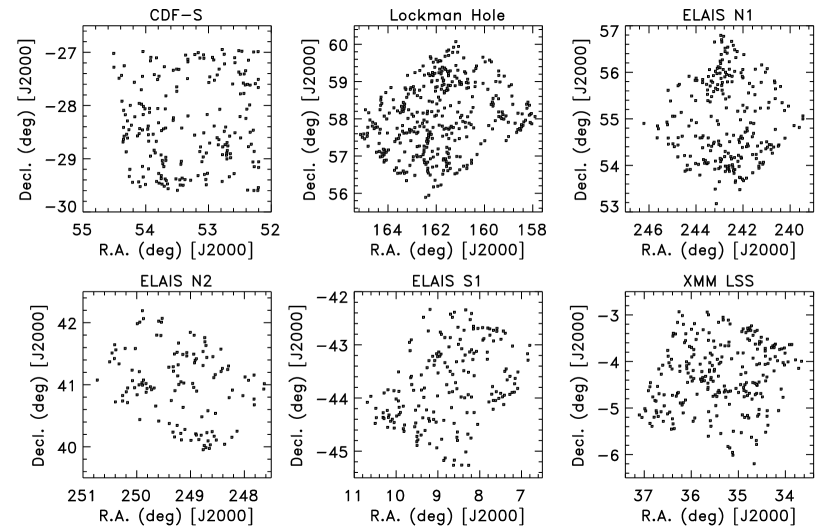
Figure 6.— The spatial distribution of galaxy cluster candidates in the six SWIRE fields (as labeled). Each data point corresponds to one cluster candidate, defined in § 3.2. Each field has very different areal coverage, see table 1. The scale of the right ascension and declination varies in each panel.

Galaxy clusters trace massive overdensities in the dark matter distribution, and thus galaxy clusters should show strong spatial clustering. We expect that the galaxy clusters defined in § 3.2 have redshifts $z\gtrsim 1$ based on their $\hbox{$[3.6]$}-\hbox{$[4.5]$}>-0.1$ mag color selection, and we use this galaxy cluster sample to study the clustering of these objects at high redshift.

Table 1Statistics on Clusters in the SWIRE fields

	Area			$\mathcal{N}$
Field	(deg2)	$\langle N(r<1\farcm 4)\rangle$	$\sigma_{N}$	(# per deg2)
(1)	(2)	(3)	(4)	(5)
CDF–S	07.8	15.4	3.9	25.2
ELAIS N1	09.3	15.3	3.8	25.9
ELAIS N2	04.2	14.9	3.6	28.6
ELAIS S1	06.8	15.5	3.8	26.7
Lockman Hole	11.1	15.6	3.9	33.2
XMM–LSS	09.1	16.0	4.0	027.3

Note. — (1) SWIRE field name, (2) IRAC data areal coverage, (3) mean number of companions with $\hbox{$[3.6]$}-\hbox{$[4.5]$}>-0.1$ mag within $r<1\farcm 4$, (4) standard deviation of clipped Gaussian of number of companions with $\hbox{$[3.6]$}-\hbox{$[4.5]$}>-0.1$ mag within $r<1\farcm 4$, (5) Surface density of galaxy clusters.

Figure 6 shows the angular distribution of the galaxy cluster samples for each of the six SWIRE fields. The angular distribution of the high redshift clusters is clearly clustered, with obvious overdensities and voids. Even though the scale of each panel in figure 6 varies somewhat, it is clear that the number density of high redshift galaxy clusters shows strong field–to–field variance, even in fields as large as those available from SWIRE ($>$5 deg²). Table 1 includes the surface densities of high–redshift galaxy clusters in the SWIRE fields. These vary from $\mathcal{N}=$25.2 deg^-2 for the CDF–S field to 33.2 deg^-2 for the Lockman Hole field. The mean surface density for all fields combined is $\langle\mathcal{N}\rangle$=28.1 deg^-2 with a standard deviation of 0.3 deg^-2 from counting statistics only. This uncertainty is significantly smaller than the field–to–field standard deviation, $\sigma_{\mathcal{N}}=2.9$ deg^-2. Therefore, the variation in the number of high redshift galaxy clusters shows substantial cosmic variance over fields as large as $\sim$10 square degrees.

We use the angular correlation function, $w(\theta)$, to quantify the clustering observed in the galaxy cluster sample, where $w(\theta)$ is the probability of finding a companion object in a solid angle $d\Omega$ at an angular separation $\theta$ in excess of a random distribution. For a distribution of sources with surface density, $\mathcal{N}$, the angular correlation function is defined as (Peebles, 1980, § 45)

$$dP=\mathcal{N}\,[1+w(\theta)]\,d\Omega.$$ (1)

The angular correlation function is calculated by comparing the total number of source pairs at a separation $\theta$ to the expected number of pairs at a separation $\theta$ from a random, uniformly distributed sample. Here we use the estimator proposed by Landy & Szalay (1993, hereafter LS), which minimizes the variance and biases associated with other estimators. The LS estimate for the angular correlation function is

$$w_{\mathrm{LS}}(\theta)=\frac{DD(\theta)-2DR(\theta)+RR(\theta)}{RR(\theta)},$$ (2)

where $DD(\theta)$ is the observed number of unique data–data pairs with angular separation $\theta-\Delta\theta/2<\theta<\theta+\Delta\theta/2$, $DR(\theta)$ is the number of unique data–random pairs in the same interval, and $RR(\theta)$ is the number of unique random–random pairs in the same interval.

As discussed by Roche & Eales (1999), because the survey fields have a finite size the expectation value for the LS estimator of the angular correlation function is biased to lower amplitudes than the true angular correlation function. It is therefore customary to correct $w_{\mathrm{LS}}(\theta)$ by adding a constant, $\mathcal{I}=w(\theta)-w_{\mathrm{LS}}(\theta)$. Following Quadri et al. (2007), this constant is equal to the fractional variance of the source counts,

$$\mathcal{I}=\frac{1}{\langle N\rangle}+\sigma^{2},$$ (3)

where $1/\langle N\rangle$ represents the Poisson error from the finite source counts, and $\sigma^{2}$ is the variance arising from object clustering in the mean density field,

$$\sigma^{2}\equiv\frac{1}{\Omega^{2}}\iint d\Omega_{1}d\Omega_{2}w(\theta_{12}).$$ (4)

Equation 4 can solved numerically if $w(\theta)$ is known (e.g., Roche & Eales, 1999). Here, we assume the angular correlation function follows the conventional power-law,

$$w(\theta)=A_{w}\theta^{-\beta},$$ (5)

for which Equation 4 becomes

$$\sigma^{2}=\frac{\sum_{i}A_{w}\theta_{i}^{-\beta}RR(\theta_{i})}{\sum_{i}RR(\theta_{i})}.$$ (6)

We solve for $A_{w}$ and $\beta$ using an iterative technique with equations 2, 3, 5, and 6. In the application to the high redshift clusters, we find that the values for $A_{w}$ and $\beta$ converge after a few iterations, and the solution appears stable in either the case where we fit for $A_{w}$ and $\beta$, or fit for only $A_{w}$ holding $\beta$ fixed (see below).

We estimate the uncertainty on $w(\theta)$ using two approaches. In the first approach, we assume the weak clustering approximation. In this case, the LS estimator has an uncertainty derived assuming Poisson variance for the data–data unique pairs, $DD$,

$$\delta w_{\mathrm{LS}}(\theta)=\frac{1+w(\theta)}{\sqrt{DD(\theta)}}.$$ (7)

The second approach uses the fact that we can derive the clustering in the six SWIRE fields independently. We then take the standard deviation of the clustering over all fields as an estimate of the error. Although in practice we find that the latter uncertainty dominates the error on the angular cluster correlation measurement, we estimate the total uncertainty by summing these two error terms in quadrature.

We calculated the angular correlation function for the high redshift galaxy clusters in the SWIRE fields using the above equations. For these calculations, we take the astrometric center of each high–redshift cluster as the mean of the astrometric locations of all galaxies assigned to that cluster. We measure the angular correlation function first for the six fields independently, and then for all six fields combined. Figure 7 shows the measured two–point angular correlation function for the high–redshift galaxy cluster candidates combined from all six SWIRE fields. The error bars on the measured amplitudes of the angular correction function correspond to the quadrature sum of the error derived from equation 7 and the standard deviation derived from the comparison of the six independent fields. However, the standard deviation between the six fields dominates the error budget.

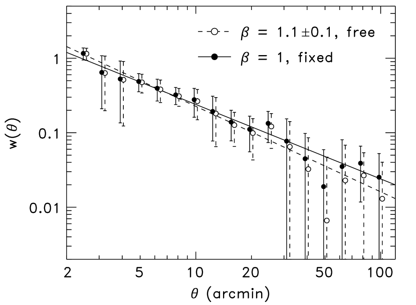
Figure 7.— The angular correlation function for the $z\gtrsim 1$ clusters measured from the six SWIRE fields. The data points show the measured angular correlation function derived assuming that $w(\theta)=A_{w}\theta^{-\beta}$, with $\beta$ as a free parameter (filled circles and solid lines) and fixed with $\beta=1.0$ (open circles and dashed lines). The data points are shifted slightly along the abscissa for clarity. The lines show the fit to these data points over $2\arcmin<\theta<100\arcmin$. The difference between the data points results from the different values for the integration constant, $\mathcal{I}$, which depend on the values of $A_{w}$ and $\beta$.

To calculate the constant, $\mathcal{I}$, we fit the function in equation 5, with $\theta$ in units of arcminutes, to the data over the interval $2\arcmin<\theta<100\arcmin$, solving first for $A_{w}$ and $\beta$ simultaneously, and then for only $A_{w}$ holding $\beta=1.0$ fixed. The choice of $\beta=1.0$ follows from measurements of the spatial correlation function of low–redshift galaxy clusters, which generally find a slope $\beta=\gamma-1\approx 1.0$, where $\xi(r)=(r/r_{0})^{-\gamma}$ (Bahcall et al., 2003). The derived value for the constant, $\mathcal{I}$, depends on the values of $A_{w}$ and $\beta$. Fitting for $A_{w}$ and $\beta$, we obtain $\mathcal{I}=0.04$, $A_{w}=3.1\pm 0.5$, and $\beta=1.1\pm 0.1$. For the case where we hold $\beta$ fixed at 1.0, we obtain $\mathcal{I}=0.05$ and $A_{w}=2.4\pm 0.2$. In all cases we derive the uncertainties on these parameters using a jackknife method (Wall & Jenkins, 2003, § 6.6), which takes into account correlations between the $w(\theta)$ datapoints. Thus, we find consistent parameters for the power-law model in either the case where we fit for $\beta$ or hold it fixed.

5. Discussion

The angular correlation function for the high–redshift clusters is consistent with a power-law fit over the interval $2\arcmin<\theta<100\arcmin$ with a power-law slope $\beta=1$. This slope corresponds to a slope for the deprojected spatial correlation function, represented by $\xi(r)=(r/r_{0})^{-\gamma}$, with $\gamma=\beta+1=2$. Such a power-law slope is representative of the correlation function of low-redshift samples of galaxy clusters (Bahcall et al., 2003, and references therein).

In this section we argue that high–redshift galaxy cluster candidates defined here correspond to the locations of mass overdensities in the large–scale structure. The selection of these objects using $\hbox{$[3.6]$}-\hbox{$[4.5]$}>-0.1$ mag from a flux–limited catalog corresponds to a specific range of redshift. In this section we calculate the redshift selection function for the high–redshift clusters. We use this to study the spatial clustering and space density of the high redshift clusters, comparing them against models for the evolution of dark matter halos.

5.1. Redshift Selection Function

To derive the redshift selection function, $dN/dz$, we make the assumption that the galaxies with $0.2<z<0.5$ make a negligible contribution to the galaxy cluster selection for the following reasons. Firstly, it is unlikely that a galaxy cluster would exist at $0.2<z<0.5$ with the requisite large number ($\geq$26 objects) of galaxies, all with substantial emission from warm dust to satisfy the IRAC color selection. Secondly, the angular diameter distance, $d_{A}$ at $z=0.35$ is roughly one–half that at $z=1.5$ (for $\Omega=0.3$ and $\Lambda=0.7$). And, by our definition (see § 3), the probability of identifying a $3\sigma$ overdensity in the surface density of red IRAC objects goes as $d_{A}^{2}$. Thus a cluster candidate composed of red IRAC objects at $0.2<z<0.5$ would require $\geq$26 (dust–enshrouded, star-forming) objects within $r\lesssim 160-250$ $h^{-1}$ kpc, i.e., a physical area $\sim$25% relative to that for $z\gtrsim 1$ objects. Such systems should be extremely rare.

Nevertheless, any contamination of low–redshift galaxy clusters in the high–redshift galaxy cluster sample will suppress the intrinsic clustering strength of the high–redshift objects. As a further test, we confirmed that the $\hbox{$[3.6]$}-\hbox{$[4.5]$}>-0.1$ mag selection excludes the relatively low–redshift ($z\lesssim 1$) X–ray selected clusters from regions of the XMM–LSS and ELAIS–S SWIRE fields with XMM coverage (Pierre et al., 2006; Puccetti et al., 2006). We select none of the 20 clusters (all with $z<1.1$) in these samples using our proposed IRAC color selection. Importantly, these samples include 11 clusters with $0.2<z<0.5$ (where we expect some contamination of galaxies with $\hbox{$[3.6]$}-\hbox{$[4.5]$}>-0.1$ mag, see § 3.1), none of which are identified by our cluster definition. Therefore, we expect a negligible contribution to the correlation function from these low–redshift clusters.

Interesting, none of the four XMM clusters with $z>0.9$ (all with $z<1.1$) would be selected by the method here. However, the selection method here does identify the projected high–redshift cluster candidates at $z=1.40-1.48$ identified by van Breukelen et al. (2007). As a further test of the redshift distribution of the IRAC–selected cluster candidates, we looked at the $\hbox{$[3.6]$}-\hbox{$[4.5]$}$ colors of the spectroscopically confirmed cluster–member galaxies in the IRAC shallow cluster survey (ISCS) with $z>1.0$ (Eisenhardt et al. 2007; M. Brodwin, private communication). Few (only 18%) of the confirmed cluster–member galaxies with $z<1.3$ have $\hbox{$[3.6]$}-\hbox{$[4.5]$}>-0.1$ mag, and these clusters would likely be missed with the selection proposed here. However, the vast majority ($\simeq$90%) of the confirmed ISCS galaxies with $z>1.3$ have $\hbox{$[3.6]$}-\hbox{$[4.5]$}>-0.1$ mag. In hindsight, the reason for this is that at $1.0<z<1.3$ the $\hbox{$[3.6]$}-\hbox{$[4.5]$}>-0.1$ mag selection misses those galaxies with passively evolving colors, which are typical of early–type galaxies. As discussed in Eisenhardt et al. (2007), nearly all the confirmed cluster galaxies in their high–redshift sample have colors consistent with older passively evolving stellar populations. The $\hbox{$[3.6]$}-\hbox{$[4.5]$}>-0.1$ mag criterion selects galaxies with the colors of these types of stellar populations for $z>1.3$ (see figure 1). Therefore, we suspect that our color selection is approximately complete for all galaxy clusters at $z>1.3$.

We estimate the broad redshift selection function for the high–redshift galaxy clusters using the observed distribution for the galaxies selected with $\hbox{$[3.6]$}-\hbox{$[4.5]$}>-0.1$ mag. We model the upper and lower end of the redshift selection function for the high–redshift galaxy clusters separately. If the majority of galaxies in clusters at $1.1<z<1.3$ have passively evolving stellar populations (as for the ISCS, see above; Eisenhardt et al. 2007), they will not be identified by our IRAC selection. Nevertheless, we conservatively assume that the redshift selection function for $1.1\lesssim z\lesssim 1.3$ follows the distribution in figure 3, and we take the spectroscopic redshift selection function for galaxies with $R>22.5$ mag and $\hbox{$[3.6]$}-\hbox{$[4.5]$}>-0.1$ mag. We furthermore correct the observed distribution using the estimated spectroscopic completeness and redshift identification completeness in the DEEP2 survey (Willmer et al., 2006). Because the galaxies in all known clusters with $z<1.1$ have colors consistent with passively evolving populations (see Eisenhardt et al., 2007, and references therein; § 1), we make the further assumption that there are no clusters at $z<1.1$ in our IRAC–selected sample.

To model the upper–end of the redshift selection function, we convert the SWIRE IRAC $[3.6]$ flux limit into the relative number of galaxies expected per unit redshift (where again, we assume the redshift selection function for the galaxy clusters is equal approximately to that of the galaxies themselves). Fontana et al. (2006) measured the evolution in the high–redshift galaxy mass function, parameterized as,

$$\phi(\mu,z)\,d\mu=2.3\,\phi^{\ast}(z)\,(10^{\mu-\mu^{\ast}[z]})^{(1+\alpha^{\ast}[z])}\exp(-10^{\mu-\mu^{\ast}[z]})\,d\mu$$ (8)

where $\mu\equiv\log(\mathcal{M})$ is the base–10 logarithm of the stellar mass, and where $\phi^{\ast}(z)\equiv\phi_{0}^{\ast}(1+z)^{\phi_{1}^{\ast}}$, $\alpha^{\ast}(z)\equiv\alpha_{0}^{\ast}+\alpha_{1}^{\ast}(z)$, and $\mu^{\ast}(z)\equiv\mu_{0}^{\ast}+\mu_{1}^{\ast}z+\mu_{2}^{\ast}z^{2}$. Fontana et al. derive best–fit parameters to their data with $\mu_{0}^{\ast}=11.16$, $\mu_{1}^{\ast}=0.17$, $\mu_{2}^{\ast}=-0.07$, $\alpha_{0}^{\ast}=-1.18$, $\alpha_{1}^{\ast}=-0.082$, $\phi_{0}^{\ast}=0.0035$, and $\phi_{1}^{\ast}=-2.20$. We calculate the number density of galaxies above some stellar mass limit and redshift integrating equation 8,

$$n(>\mathcal{M},z)=\int_{\log\mathcal{M}}^{\hbox{$\infty$}}\phi(\mu,z)\,d\mu.$$ (9)

We convert equation 9 into the number of galaxies above the IRAC flux limit for SWIRE as a function of redshift using an estimate for the galaxy mass–to–light ratio, $\mathcal{M}/L_{\nu}(z)$, where $L_{\nu}(z)$ is the luminosity density at 3.6/(1+$z$) µm. Here, we take $f_{\mathrm{lim}}(3.6\micron)=7$ $\mu$Jy as the flux limit. The observed mass–to–light ratio depends on the relative number of early– and late–type stellar populations constituting each galaxy (e.g., Bruzual & Charlot, 2003) and dust extinction. However, Rudnick et al. (2006) showed that the global galaxy population at $0.7<z<2.5$ has rest–frame $U-B$ and $B-V$ colors consistent with a simple exponentially declining star-formation rate with a characteristic timescale of 6 Gyr, formed at $z_{\mathrm{form}}=4$ with dust extinction of $A_{V}=0.6$ mag. We therefore use a stellar population model (from Bruzual & Charlot, 2003) with these parameters to compute $\mathcal{M}/L_{\nu}(z)$. The limiting mass as a function of redshift is then $\mathcal{M}_{\mathrm{lim}}=\mathcal{M}/L_{\nu}(z)\times f_{\mathrm{lim}}(3.6\micron)\times 4\pi D_{L}^{2}(z)(1+z)^{-1}$, where $D_{L}(z)$ is the luminosity distance. We insert this expression into equation 9. The redshift distribution function is then the derivative of equation 9 with respect to redshift, $dN/dz=dn(>\mathcal{M}_{\mathrm{lim}},z)/dz$.

The intersection of the lower– and upper–end of the redshift selection functions yields the total redshift selection function. Figure 8 shows the total redshift selection function and the individual components. We normalize the redshift selection function with the convention, $\int dN/dz\;\;dz=1$. The mean and variance of the redshift distribution function are the first and second moments of this distribution, which give $\langle z\rangle=1.54$ and $\sigma(z)=\sqrt{\sigma^{2}}=0.28$.

We use the redshift selection function to estimate the spatial number density of the galaxy clusters. The number density is equal to

$$n=\frac{\mathcal{N}}{\int(1+z)^{2}\,p(z)\,d_{A}^{2}\,E(z)^{-1}\,dz},$$ (10)

where $\mathcal{N}$ is the observed surface density, and we define the function (Peebles, 1993, pgs. 100, 312, 332)

$$E(z)=\left(\frac{c}{H_{0}}\right)^{-1}[\Omega_{m}(1+z)^{3}+\Omega_{R}(1+z)^{2}+\Omega_{\Lambda}]^{1/2},$$ (11)

where $\Omega_{R}=1-\Omega_{m}-\Omega_{\Lambda}\equiv 0$ here. The denominator of equation 10 is the effective volume per unit solid angle. The effective volume differs from the comoving volume by $p(z)$, which is the probability that a cluster with redshift $z$ will be selected using the method here, thus $0\leq p(z)\leq 1$ for all $z$. The quantity $p(z)$ compensates for various selection biases and incompleteness. We generally assume here that $p(z)\propto dN/dz$ with a normalization such that $p(z)=1.0$ for $1.3<z<1.5$. However, the completeness is poorly known given the relatively complicated selection function for the high–redshift clusters (see above). Therefore, in the discussion that follows we also consider other distributions for $p(z)$ that should span the possible plausible range. This provides limits on the effective volume for the high–redshift clusters until improvements in the selection function become available (either from spectroscopic or accurate photometric redshifts).

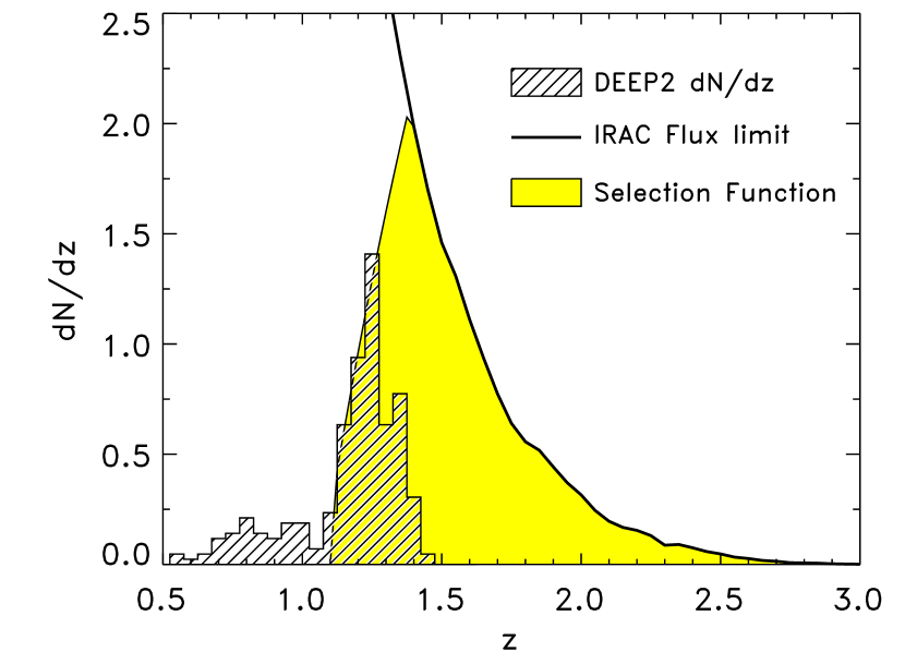
Figure 8.— The redshift selection function for high redshift galaxy clusters selected from the SWIRE data with $\hbox{$[3.6]$}-\hbox{$[4.5]$}>-0.1$ mag. The hashed histogram shows the spectroscopic redshift distribution of DEEP2 galaxies with $\hbox{$[3.6]$}-\hbox{$[4.5]$}>-0.1$ mag, $R>22.5$ mag, and IRAC flux densities above the SWIRE limit, which represents the lower–end of the redshift selection function. The thick solid line shows the expected redshift distribution of IRAC sources to the SWIRE flux limit with assumptions on the evolution of the mass function and color distribution of galaxies (see text), and this represents the upper–end of the redshift selection function. The intersection of the lower– and upper–end of the redshift selection functions provides the total redshift selection function, $dN/dz$, which is indicated by the yellow–shaded region.

Applying equation 10 to the redshift selection function with the numbers in table 1, the spatial number density of the high redshift galaxy clusters is $n=1.2\pm 0.1\times 10^{-5}\,h^{3}$ Mpc^-3, where the uncertainty is the standard deviation on the spatial densities derived separately for the six SWIRE fields. However, the number density dependent on the assumed redshift selection function, which we discuss further in § 5.3.

5.2. Spatial Clustering of High Redshift Clusters

The angular correlation function, $w(\theta)$, corresponds to the 3–dimensional spatial correlation function, $\xi(r)$, projected on sky. They are related through the Limber projection using a known redshift selection function, $dN/dz$ (Efstathiou et al., 1991; Peebles, 1980, § 50, 52). Allowing the evolution of the spatial correlation function to follow, $\xi(r,z)=\xi(r,0)\times f(z)$, where $\xi(r,0)=(r/r_{0})^{-\gamma}$ as above, and conventionally $f(z)=(1+z)^{-(3-\gamma+\epsilon)}$, then the relation between the amplitude of the angular correlation function and the spatial correlation function is (Efstathiou et al., 1991)

$$A_{w}=H_{\gamma}\,r^{\gamma}_{0}\,\int f(z)\,d_{C}^{1-\gamma}(z)\,\left(\frac{dN}{dz}\right)^{2}E(z)dz\,\,\left(\int\frac{dN}{dz}dz\right)^{-2},$$ (12)

where $d_{C}$ is the comoving distance, $dN/dz$ is the redshift selection function, $E(z)$ is defined in equation 11, and $H_{\gamma}$ is a numerical factor given by (Peebles, 1980, § 52)

$$H_{\gamma}=\sqrt{\pi}\frac{\Gamma[(\gamma-1)/2]}{\Gamma(\gamma/2)}.$$ (13)

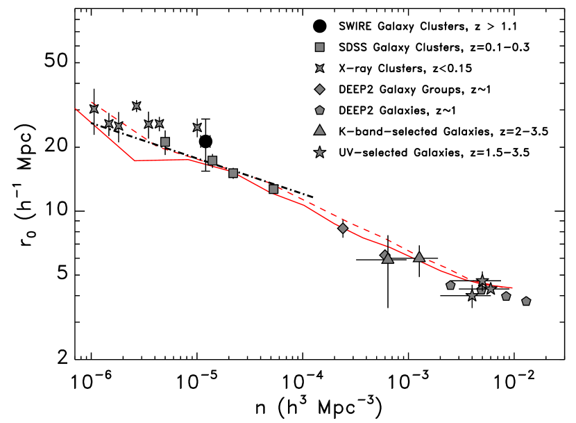
Figure 9.— The comoving number density, $n$, versus the spatial correlation function scale length, $r_{0}$, for various objects at different redshifts. The large, filled circle shows the value derived here for the IRAC–selected high–redshift cluster candidates, assuming the redshift distribution in figure 8, and includes an additional systematic error (summed in quadrature) of $\delta(r_{0})=5$ $h^{-1}$ Mpc for uncertainties in the redshift selection function. The filled squares show optically-selected galaxy clusters from SDSS with $N_{\mathrm{gal}}>10$, 13, 15, and 20 from Bahcall et al. (2003). The four–point stars show X-ray–selected galaxy clusters with $L_{X}\gtrsim 10^{43}$ erg s^-1 (Abadi et al., 1998; Lee & Park, 1999; Collins et al., 2000; Bahcall et al., 2003). Filled pentagons show the $z\sim 1$ galaxy sample from DEEP2 (Coil et al., 2006a), and filled diamonds show the $z\sim 1$ galaxy–group sample from DEEP2 (Coil et al., 2006b). The filled triangles show $K$–band selected galaxies at $z\sim 2$ from Quadri et al. (2007). The filled pentagrams show UV–selected “U–dropouts” at $1.5<z<2.0$, $2.0<z<2.5$, and $2.5<z<3.5$ from Adelberger et al. (2005). The lines show various models. The dot–dashed line shows the empirical relation $r_{0}\sim 2.6n^{-3/2}$ derived for a $\Lambda$CDM model used by Bahcall et al. (2003). The red lines show predictions from the Millennium model simulations for $z=0.2$ (solid line) and $z=1.5$ (dashed line).

Following the arguments of Giavalisco et al. (1998), for the large spatial scales considered here the effective variation in the correlation length, $r_{0}$, should be small. Therefore, we take $\epsilon=\gamma-3$, corresponding to constant clustering in comoving units over the redshift range considered here. In this case, $r_{0}(z)=r_{0}$ is the correlation length at the epoch of the observation.

We solve equation 12 for the spatial correlation scale length, $r_{0}$, using the redshift selection function derived in § 5.1 (see figure 8), and $A_{w}$ and $\beta$ derived for the angular correlation function in § 4. For the case where $\beta=1.0$ ($A_{w}=2.4\pm 0.2$), we derive $r_{0}=26.9\pm 5.6$ $h^{-1}$ Mpc. For the case where $\beta$ varies ($A_{w}=3.1\pm 0.5$ and $\beta=1.1\pm 0.1$), we derive $r_{0}=22.4\pm 3.6$ $h^{-1}$ Mpc. Because these two cases give consistent answers, we quote here the value for the latter, which includes the larger error and is thus more conservative.

Figure 9 illustrates the relation of $r_{0}$ to the spatial density, $n$, for the high–redshift galaxy clusters discussed here to other samples in the literature. The spatial correlation scale length for the high–redshift galaxy clusters is comparable to that derived for optically–selected rich clusters at relatively low redshift ($0.1<z<0.3$, Bahcall et al., 2003). This implies that the high–redshift galaxy clusters selected by IRAC are progenitors of low–redshift galaxy clusters. The spatial correlation function scale length is also consistent with those derived for luminous X-ray clusters ($L_{X}\gtrsim 10^{43}$ erg s^-1), which range from $r_{0}\sim 25-30$ $h^{-1}$ Mpc (Abadi et al., 1998; Lee & Park, 1999; Collins et al., 2000, with values taken from Bahcall et al. 2003). Therefore, some of the high–redshift galaxy clusters seem destined to become luminous X–ray clusters.

The largest uncertainty in the derived spatial correlation scale length stems from the assumed shape of the redshift selection function, $dN/dz$. In particular, our redshift selection function is fairly broad and assumes the clusters are smoothly distributed over $1.1<z\lesssim 3.0$. If the clusters show prominent, discrete voids and spikes in this distribution, this will lower the spatial correlation scale length (Adelberger, 2005). However, because we average the correlation functions over the six separate SWIRE fields, we expect this effect is less severe. Larger uncertainties likely result from the cluster galaxy colors and from the fact that the redshift distribution of bona fide high–redshift galaxy clusters may not be equal to that of the general galaxy population. For example, one extreme (yet very possible) scenario is that galaxies in all clusters with $1.1<z<1.5$ have colors consistent with passively evolving stellar populations. In this case, the IRAC $\hbox{$[3.6]$}-\hbox{$[4.5]$}>-0.1$ mag selection would miss all clusters with $z<1.3$, like those in the ISCS discussed above (see § 5.1; Eisenhardt et al., 2007). Furthermore, if the redshift distribution of galaxy clusters evolves more strongly at high redshifts than the general galaxy population, then the redshift selection function in figure 8 would over predict the number of clusters with $z\gtrsim 1.5$.

All the effects discussed above would narrow the redshift selection function compared to that derived in § 5.1, which would lower the derived spatial correlation function scale length. As a fiducial example, inserting a redshift selection function described by a Gaussian, $dN/dz\propto\exp(-(z-\bar{z})^{2}/2\sigma_{z}^{2})$ with $\bar{z}=1.5$ and $\sigma_{z}=0.1$, would reduce the spatial correlation function scale length to $r_{0}\approx 18$ $h^{-1}$ Mpc (consistent with the $r_{0}$ derived for $\langle z\rangle=1$ clusters in the ISCS, see Brodwin et al. 2007). Therefore, we incorporate the uncertainty on the redshift selection function by adding (in quadrature) an additional error $\delta(r_{0})=5$ $h^{-1}$ Mpc to the correlation length in figure 9. However, this error is systematic, and its general effect is to lower the derived value of $r_{0}$. Such a redshift selection function would also increase the number density derived in equation 10 to $\approx 2\times 10^{-5}$ $h^{3}$ Mpc^-3. To remove this source of systematic uncertainty requires deriving a more accurate redshift selection function, either through spectroscopy or with good photometric redshifts. The data required to estimate a more accurate redshift selection function do not yet exist over the full SWIRE fields.

Current large–scale cosmological simulations using an $\Lambda$CDM model reproduce the comoving clustering and space density of the galaxy clusters, groups, and galaxies. Figure 9 shows a fit to the $\Lambda$CDM model invoked by Bahcall et al. (2003), $r_{0}\sim 2.6n^{-3/2}$, over the range $20<n^{-1/3}<90\,h^{-1}$ Mpc. This model intersects the optically-selected clusters, although it corresponds to values or $r_{0}$ lower than those measured for the less-luminous X-ray clusters. Similarly, recent cosmological models from the Millennium simulation (Springel et al., 2005) reproduce the data on scales from galaxy clusters to the galaxies themselves. The two curves in the figure show the Millennium–simulation predictions for $z=0.2$ and 1.5. The model predictions show the relationship between the clustering strength and space density of dark–matter halos. Therefore, the measured clustering of galaxy clusters, galaxy groups, and galaxies implies that these objects trace the underlying dark matter halos over a large range of mass scale and redshift.

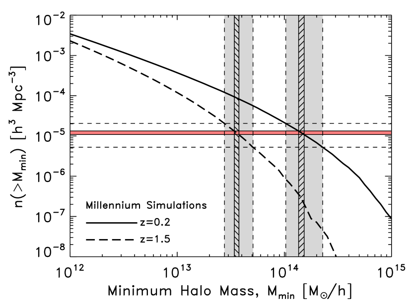
Figure 10.— Number density of dark matter halos as a function of halo mass. The curves show the expected number density of halos greater than mass, $\mathcal{M}$, for $z=0.2$ (solid lines) and $z=1.5$ (dashed lines) from the Millennium model simulations (Springel et al., 2005). The shaded horizontal band shows the measured number density of galaxy clusters at $z\gtrsim 1$ from SWIRE assuming the fiducial redshift selection function derived in § 5.1. The horizontal short-dashed lines show the bound on the number density for limiting cases in the assumed redshift selection function. The vertical hashed regions show masses to which the measured number density corresponds at each redshift, and the shaded region extends these for the limiting number densities. While the measured number density corresponds to a halo mass of $\approx 3-5\times 10^{13}\;h^{-1}$ $\mathcal{M}_{\odot}$ at $z=1.5$, these will evolve to have halo masses of $\approx 1-3\times 10^{14}\;h^{-1}$ $\mathcal{M}_{\odot}$ at $z=0.2$.

5.3. Evolution of Galaxy Clusters

The cosmological simulations match the behavior of the number density and spatial correlation function scale length of the high–redshift galaxy clusters. Thus, we may relate the derived number density for the high–redshift galaxy clusters to estimate the corresponding dark matter halo mass in the simulations. Figure 10 shows the expected number distribution of dark–matter halos above a given mass threshold at $z=1.5$ and 0.2 for the Millennium simulation (Springel et al., 2005). At $z=1.5$, near the mean redshift of our redshift distribution function (§ 5.1), the comoving number density of the IRAC–selected high–redshift galaxy clusters corresponds to dark matter halos larger than $3.5\times 10^{13}$ $h^{-1}$ $\mathcal{M}_{\odot}$.

As discussed in § 5.2, the number density is uncertain due to the unknown redshift selection function. In the discussion here, we allow for two limiting redshift selection functions to constrain the range for the comoving number density, and thus the range of dark matter halo masses. The first limiting number density corresponds to the case where the redshift selection function is represented by a Gaussian with $\langle z\rangle$=1.5 and $\sigma_{z}=0.1$. In this case the number density would increase to $2\times 10^{-5}$ $h^{3}$ Mpc^-3. Alternatively, we consider the case where the redshift selection function is constant for $1.1<z<2.5$ and zero elsewhere. In this case, the number density would decrease to $3\times 10^{-6}$ $h^{3}$ Mpc^-3. These cases are arguably limiting cases, and thus they bound the range of possible comoving number densities. Figure 10 shows the number densities for these cases, and these would correspond to dark matter haloes at $z=1.5$ larger than $\approx$$3-5\times 10^{13}$ $h^{-1}$ $\mathcal{M}_{\odot}$.

Due to hierarchical nature of CDM, these objects continue to accrete matter with decreasing redshift. Figure 10 shows that the range of comoving number densities for the IRAC–selected galaxy clusters at $z\gtrsim 1$ correspond to dark matter halos larger than $1-3\times 10^{14}$ $h^{-1}$ $\mathcal{M}_{\odot}$ at $z=0.2$, which is comparable to the dark–matter halo masses of the SDSS optically-selected clusters (Bahcall et al., 2003) and X-ray clusters (Abadi et al., 1998; Collins et al., 2000).

Therefore, the high–redshift galaxy clusters identified by the $\hbox{$[3.6]$}-\hbox{$[4.5]$}>-0.1$ mag selection correspond to rich present–day clusters. This is perhaps unsurprising given that we defined the high–redshift clusters to have $\geq$26–28 companions within angular sizes of 1.4 arcminutes. Presumably the number density (and spatial clustering correlation length) depends on this definition. Requiring a larger number of galaxies within this aperture would identify rarer objects with a lower number density, perhaps identifying the denizens of larger–mass dark matter halos. Similarly, requiring a smaller number of galaxies presumably corresponds to lower–mass halos, although using a smaller number of galaxies will also suffer more from contamination from the average surface density for objects with $\hbox{$[3.6]$}-\hbox{$[4.5]$}>-0.1$ mag unassociated with galaxy clusters.

It is worth noting that the high–redshift galaxy clusters defined here are relatively unbiased by the (rest–frame) optical colors of the galaxies. They have no dependence on any color other than $\hbox{$[3.6]$}-\hbox{$[4.5]$}$. Therefore, measuring the distribution of rest–frame optical colors in the galaxies of these clusters will allow the study of when and how these objects formed their stellar populations. However, to derive accurate rest–frame colors requires more accurate redshift estimates than what is possible with only the $\hbox{$[3.6]$}-\hbox{$[4.5]$}$ color and the redshift selection function in § 5.1, and good redshifts (photometric or spectroscopic) are needed for further study of the colors of the galaxies in these clusters. Unfortunately, the current optical imaging with the public SWIRE data release covers only $\approx$30% of the area of the IRAC survey (and not all of these data are useful for photometric redshifts). More ancillary data will be required to study the evolution of the galaxies in the high–redshift IRAC–selected clusters, and to compare them to the galaxies in lower redshift galaxy clusters.

6. Summary

We discuss the angular clustering of galaxy clusters at $z>1$ selected over 50 deg² from SWIRE. We select high–redshift galaxies ($z\gtrsim 1$) using a simple color selection, $\hbox{$[3.6]$}-\hbox{$[4.5]$}>-0.1$ mag. The small number of contaminants may be rejected using an additional apparent magnitude limit $R>22.5$ mag, which efficiently removes galaxies with $0.2<z<0.5$.

From the galaxies with $\hbox{$[3.6]$}-\hbox{$[4.5]$}>-0.1$ mag, we identify galaxy cluster candidates as objects with $\geq$26–28 companions within $r=1\farcm 4$ radii. Using datasets with high–quality spectroscopic redshifts, we show that the majority ($>$80%) of all galaxies satisfying $(\hbox{$[3.6]$}-\hbox{$[4.5]$})_{\mathrm{AB}}>-0.1$ mag have $z>1.0$. Furthermore, more than 50% (90%) of the galaxies with spectroscopic redshifts $z>1.1$ (1.3) satisfy this IRAC color selection.

These candidate galaxy clusters show strong angular clustering. From the data, we derived an angular correlation function represented by $w(\theta)=(3.1\pm 0.5)(\theta/1\arcmin)^{-1.1\pm 0.1}$ over scales of 2–100 arcmin. The slope of the angular correlation function, $\beta$, corresponds to a slope of the spatial correlation function $\gamma=\beta+1\simeq 2.0$, consistent with the slope for low–redshift galaxy clusters.

Assuming the redshift distribution of these galaxy clusters follows our fiducial model, these galaxy clusters have a spatial–clustering scale length $r_{0}=22.4\pm 3.6h^{-1}$ Mpc, and a number density $1.2\pm 0.1\times 10^{-5}h^{3}$ Mpc^-3. The correlation scale length and number density of these objects are comparable to those of rich optically–selected and X-ray–selected galaxy clusters at low redshift. However, the largest uncertainty on the spatial–clustering scale length stems from uncertainties in the redshift selection function. The $\hbox{$[3.6]$}-\hbox{$[4.5]$}>-0.1$ mag selection would miss the galaxies in clusters at $1.1<z<1.3$, if these clusters are dominated by galaxies with colors consistent with passively evolving stellar populations. Furthermore, if the redshift distribution of galaxy clusters evolves more strongly at high redshifts than the general galaxy population, then our redshift selection function would over predict the number of clusters at the highest redshifts. These effects would narrow the redshift selection function, which would tend to lower the spatial correlation function scale length. To improve the measurement on the spatial correlation function requires a more accurate redshift selection function, either from deep spectroscopy or well–calibrated photometric redshifts.

Comparing the number density of these high–redshift clusters to dark–matter halos from the $\Lambda$CDM Millennium simulations, the high–redshift clusters correspond to dark–matter halos larger than $3-5\times 10^{13}$ $h^{-1}$ $\mathcal{M}_{\odot}$ at $z=1.5$, including an allowance for the possible range of number densities. Assuming these grow following $\Lambda$CDM models, these clusters will reside in halos larger than $1-3\times 10^{14}$ $h^{-1}$ $\mathcal{M}_{\odot}$ at $z=0.2$, comparable to large galaxy clusters at low redshift. Therefore, the IRAC–selected galaxy clusters correspond to the high–redshift progenitors of present–day galaxy clusters.

The selection of the high–redshift galaxy clusters has no dependence on the rest–frame optical colors of the galaxies themselves. Therefore, future observations of the galaxies in these high–redshift galaxy clusters allows the study of their star–formation histories with little additional bias.

References

- Abadi et al. (1998) Abadi, M. G., Lambas, D. G., & Muriel, H. 1998, ApJ, 507, 526
- Adelberger (2005) Adelberger, K. L. 2005, ApJ, 621, 574
- Adelberger et al. (2005) Adelberger, K. L., Steidel, C. C., Pettini, M., Shapley, A. E., Reddy, N. A., & Erb, D. K. 2005, ApJ, 619, 697
- Alexander et al. (2003) Alexander, D. M. et al. 2003, AJ, 126, 539
- Bahcall (1988) Bahcall, N. A. 1988, ARA&A, 26, 631
- Bahcall et al. (2003) Bahcall, N. A., Dong, F., Hao, L., Bode, P., Annis, J., Gunn, J. E., & Schneider, D. P. 2003, ApJ, 599, 814
- Barmby et al. (2007) Barmby, P., Huang, J.–S., Ashby, M. L. N., Eisenhardt, P. R. M., Fazio, G. G., Willner, S. P., & Wright, E. L. ApJ, submitted
- Brodwin et al. (2006) Brodwin, M., et al. 2006, ApJ, 651, 791
- Brodwin et al. (2007) Brodwin, M., et al. 2007, ApJ, in press (astro-ph/0711.1863)
- Bruzual & Charlot (2003) Bruzual, G. A., & Charlot, S. 2003, MNRAS, 344, 1000
- Calzetti et al. (2000) Calzetti, D., Armus, L., Bohlin, R. C., Kinney, A. L., Koornneef, J., & Storchi-Bergmann, T. 2000, ApJ, 533, 682
- Coil et al. (2006a) Coil, A. L., Newman, J. A., Cooper, M. C., Davis, M., Faber, S. M., Koo, D. C., & Willmer, C. N. A. 2006a, ApJ, 644, 671
- Coil et al. (2006b) Coil, A. L., et al. 2006b, ApJ, 638, 668
- Collins et al. (2000) Collins, C. A., et al. 2000, MNRAS, 319, 939
- Cooper et al. (2007) Cooper, M. C., et al. 2007, MNRAS, 376, 1445
- Croft et al. (2005) Croft, S., Kurk, J., van Breugel, W., Stanford, S. A., de Vries, W., Pentericci, L., Röttgering, H. 2005, AJ, 130, 867
- Davis et al. (2007) Davis, M., et al. 2007, ApJ, 660, L1
- Dickinson et al. (2003) Dickinson, M., et al. 2003, in The Mass of Galaxies at Low and High Redshift, ed. R. Bender & A. Renzini, (Berlin: Springer), 324
- Dressler (1980) Dressler, A. 1980, ApJ, 236, 351
- Efstathiou et al. (1991) Efstathiou, G., Bernstein, G., Tyson, J. A., Katz, N., & Guhathakurta, P. 1991, ApJ, 380, L47
- Eisenhardt et al. (2007) Eisenhardt, P. R. M., et al. 2007, ApJ, submitted
- Elbaz et al. (2007) Elbaz, D., et al. 2007, A&A, 468, 33
- Fontana et al. (2006) Fontana, A., et al. 2006, A&A, 459, 745
- Gerke et al. (2007) Gerke, B. F., et al. 2007, MNRAS, 376, 1425
- Giavalisco et al. (1998) Giavalisco, M., Steidel, C. C., Adelberger, K. L., Dickinson, M. E., Pettini, M., & Kellogg, M. 1998, ApJ, 503, 543
- Giavalisco et al. (2004) Giavalisco, M., et al. 2004, ApJ, 600, L93
- Gladders & Yee (2005) Gladders, M. D., & Yee, H. K. C. 2005, ApJS, 157, 1
- Gladders et al. (2007) Gladders, M. D., Yee, H. K. C., Majumdar, S., Barrientos, L. F., Hoekstra, H., Hall, P. B., & Infante, L. 2007, ApJ, 655, 128
- Gonzalez et al. (2002) Gonzalez, A. H., Zaritsky, D., & Wechsler, R. H. 2002, ApJ, 571, 129
- Imanishi et al. (2006) Imanishi, M., Dudley, C. C., & Maloney, P. R. 2006, ApJ, 637, 114
- Haiman, Mohr, & Holder (2001) Haiman, Z., Mohr, J. J., & Holder, G. P. 2001, ApJ, 553, 545
- Kajisawa et al. (2006) Kajisawa, M., Kodama, T., Tanaka, I., Yamada, T., & Bower, R. 2006, MNRAS, 371, 577
- Kitayama & Suto (1996) Kitayama, T., & Suto, Y. 1996, ApJ, 469, 480
- Kodama et al. (2007) Kodama, T., Tanaka, I., Kajisawa, M., Kurk, J., Venemans, B., De Breuck, C., Vernet, J., & Lidman, C. 2007, MNRAS, 377, 1717
- Kurk et al. (2000) Kurk, J. D., et al. 2000, A&A, 358, L1
- Landy & Szalay (1993) Landy, S. D., & Szalay, A., S. 1993, ApJ, 412, 64 (LS)
- Le Fèvre et al. (2004) Le Fèvre, O., et al. 2004, A&A, 428, 1043
- Lee & Park (1999) Lee, S. & Park, C. 1999, J. Korean Astron. Soc., 32, 1
- Lonsdale et al. (2003) Lonsdale, C. J., et al. 2003, PASP, 115, 897
- Lubin et al. (1998) Lubin, L. M., Postman, M., Oke, J. B., Ratnatunga, K. U., Gunn, J. E., Hoessel, J. G., & Schneider, D. P. 1998, AJ, 116, 584
- Maraston (2005) Maraston, C. 2005, MNRAS, 362, 799
- McCarthy et al. (2007) McCarthy, P. J., et al. 2007, ApJ, 664, L17
- Mignoli et al. (2005) Mignoli, M., et al. 2005, A&A, 437, 883
- Miley et al. (2004) Miley, G. K., et al. 2004, Nature, 427, 47
- Mullis et al. (2005) Mullis, C. R., Rosati, P., Lamer, G., Böhringer, H., Schwope, A., Schuecker, P., & Fassbender, R. 2005, ApJ, 623, L85
- Nandra et al. (2005) Nandra, K., et al. 2005, MNRAS, 356, 568
- Peebles (1980) Peebles, P. J. E. 1980, The Large-Scale Structure of the Universe (Princeton: Princeton University Press)
- Peebles (1993) Peebles, P. J. E. 1993, Principles of Physical Cosmology (Princeton: Princeton University Press)
- Pierre et al. (2006) Pierre, M., et al. 2007, A&A, 2006, 372, 591
- Postman et al. (1998) Postman, M., Lubin, L. M., & Oke, J. B. 1998, AJ, 116, 560
- Puccetti et al. (2006) Puccetti, S., et al. 2006, A&A, 2006, 457, 501
- Quadri et al. (2007) Quadri, R., et al. 2007, ApJ, 654, 138
- Reddy et al. (2006) Reddy, N. A., Steidel, C. C., Erb, D. K., Shapley, A. E., & Pettini, M. 2006, ApJ, 653, 1004
- Roche & Eales (1999) Roche, N., & Eales, S. A. 1999, MNRAS, 307, 703
- Rosati et al. (2002) Rosati, P., Borgani, S., & Norman, C. 2002, ARA&A, 40, 539
- Rosati et al. (2004) Rosati, P., et al. 2004, AJ, 127, 230
- Rudnick et al. (2006) Rudnick, G., et al. 2006, ApJ, 650, 624
- Sawicki (2002) Sawicki, M. 2002, AJ, 124, 3050
- Shapley et al. (2005) Shapley, A. E., Steidel, C. C., Erb, D. K., Reddy, N. A., Adelberger, K. L., Pettini, M., Barmby, P., & Huang, J. 2005, ApJ, 626, 698
- Simpson & Eisenhardt (1999) Simpson, C., & Eisenhardt, P. 1999, PASP, 111, 691
- Springel et al. (2005) Springel, V., et al. 2005, Nature, 435, 629
- Stanford, Eisenhardt, & Dickinson (1998) Stanford, S. A., Eisenhardt, P. R. M., & Dickinson, M. 1998, ApJ, 492, 461
- Stanford et al. (2005) Stanford, S. A., et al. 2005, ApJ, 634, L129
- Stanford et al. (2006) Stanford, S. A., et al. 2006, ApJ, 646, L13
- Steidel et al. (1998) Steidel, C. C., Adelberger, K. L., Dickinson, M., Giavalisco, M., Pettini, M., & Kellogg, M. 1998, ApJ, 492, 428
- Steidel et al. (2005) Steidel, C. C., Adelberger, K. L., Shapley, A. E., Erb, D. K., Reddy, N. A., & Pettini, M. 2005, ApJ, 626, 44
- Stern et al. (2003) Stern, D., Holden, B., Stanford, S. A., & Spinrad, H. 2003, AJ, 125, 2759
- Stern et al. (2005) Stern, D., et al. 2005, ApJ, 631, 163
- Surace et al. (2005) Surace, J. A., et al. 2005, BAAS, 37, 1246
- Szokoly et al. (2004) Szokoly, G. P., et al. 2004, ApJS, 155, 271
- Takagi et al. (2007) Takagi, T., et al. 2007, PASJ, in press (astro-ph/0705.1365)
- van Breukelen et al. (2006) van Breukelen, C., et al. 2006, MNRAS, 373, L26
- van Breukelen et al. (2007) van Breukelen, C., et al. 2007, MNRAS, 382, 971
- van Dokkum et al. (2007) van Dokkum, P. G., Cooray, A., Labbé, I., Papovich, C., & Stern, D., 2007, preprint (astro-ph/0709.0946)
- van Dokkum & Franx (2001) van Dokkum, P. G., & Franx, M. 2001, ApJ, 553, 90
- van Dokkum et al. (2000) van Dokkum, P. G., Franx, M., Fabricant, D., Illingworth, G. D., & Kelson, D. D. 2000, ApJ, 541, 95
- van Dokkum & van der Marel (2007) van Dokkum, P. G., & van der Marel, R. P. 2007, ApJ, 655, 30
- Vanzella et al. (2005) Vanzella, E., et al. 2005, A&A, 434, 53
- Vanzella et al. (2006) Vanzella, E., et al. 2006, A&A, 454, 423
- Venemans et al. (2002) Venemans, B. P., et al. 2002, ApJ, 569, L11
- Venemans et al. (2007) Venemans, B. P., et al. 2007, A&A, 461, 823
- Wall & Jenkins (2003) Wall, J. V., & Jenkins, C. R. 2003, Practical Statistics for Astronomers (Cambridge: Cambridge University Press)
- Wang & Steinhardt (1998) Wang, L., & Steinhardt, P. J. 1998, ApJ, 508, 483
- Willmer et al. (2006) Willmer, C. N. A., et al. 2006, ApJ, 647, 853
- Wilson et al. (2006) Wilson, G., et al. 2006, in Infrared Diagnostics of Galaxy Evolution, ed. R. Chary (San Francisco: ASP), in press (astro-ph/0604289)
- Zehavi et al. (2004) Zehavi, I., et al. 2004, ApJ, 608, 16