Higher derivative regularization and quantum corrections in $N=1$ supersymmetric theories.

Abstract

We review some results of applying the higher covariant derivative regularization to the investigation of quantum corrections structure in $N=1$ supersymmetric theories. In particular, we demonstrate that all integrals, defining the Gell-Mann–Low function in supersymmetric theories, are integrals of total derivatives. As a consequence, there is an identity for Green functions, which does not follow from any known symmetry of the theory, in $N=1$ supersymmetric theories. We also discuss how to derive the exact $\beta$-function by methods of the perturbation theory.

1 Introduction.

Supersymmetry is certainly one of the most prominent achievements of the high energy physics. Soon after its discovery it was found that in supersymmetric theories the ultraviolet behavior was essentially improved due to some non-renormalization theorems. For example, there are no divergences in the $N=4$ supersymmetric Yang–Mills theory, and in theories with $N=2$ supersymmetry divergences are present only in the one-loop approximation. That is why such models are very attractive from the theoretical point of view. But, possibly, the most interesting fact is an indirect experimental proof of supersymmetry existence in the Standard model. It was obtained by precise measuring three coupling constants and investigating their evolution by the renormgroup equations. The result is that only in the supersymmetric version of the Standard model the coupling constants coincide at some energy scale, which should follow from Grand Unification theories. So, there is no doubt that investigating supersymmetric theories and, in particular, their quantum properties, is very interesting. Dynamics of supersymmetric theories is highly nontrivial. It is worth mentioning summation of instanton corrections in the $N=2$ supersymmetric Yang–Mills theory [1] (see also [2, 3, 4, 5]) or finding a relation between the $N=4$ supersymmetric Yang–Mills theory and a string theory, compactified on the manifold $AdS_{5}\times S_{5}$, known as the AdS/CFT-correspondence [6].

In this paper we will consider theories with unextended supersymmetry. Such models are especially interesting, because the physics seems to be $N=1$ supersymmetric at energies of the order $10^{3}$ GeV. Dynamics of $N=1$ supersymmetric theories also has some interesting features. For example, as a result of investigating instanton contributions structure, in Ref. [7] form of the $\beta$-function was suggested exactly to all orders of the perturbation theory. This $\beta$-function, called the exact Novikov–Shifman–Vainshtein–Zakharov (NSVZ) $\beta$-function is

$$\beta(\alpha)=-\frac{\alpha^{2}\Big{[}3C_{2}-C(R)\Big{(}1-\gamma(\alpha)\Big{)}\Big{]}}{2\pi(1-C_{2}\alpha/2\pi)},$$ (1)

where $\gamma(\alpha)$ is the anomalous dimension of the matter superfield in a representation $R$, and $C(R)$ is defined by

$$\mbox{tr}\,(T^{a}T^{b})=C(R)\,\delta^{ab}.$$ (2)

Such a $\beta$-function has not yet been derived by methods of the perturbation theory. Its numerous verifications by explicit calculations up to the four-loop approximation were made in Refs. [8, 9, 10]. The authors calculated the $\beta$-function, defined by divergence in the $\overline{MS}$-scheme. The main result is the following: if a subtraction scheme is tuned by a special way, then it is possible to obtain the exact NSVZ $\beta$-function. Nevertheless, there is an open question, in which scheme one can obtain this $\beta$-function. The answer to this question is, in particular, given in this paper. Moreover, we show that there are new identities, relating Green functions in some $N=1$ supersymmetric theories, which do not follow from known symmetries of the theory. Possibly, this assumes existence of some new invariances. Note that possibility of their existence was discussed, for example, in finite $N=1$ supersymmetric theories [11]. Thus, the dynamics of $N=1$ supersymmetric theories is highly nontrivial and deserves further investigation. An important constituent of this investigation is a regularization [12]. The matter is that the dimensional regularization [13] breaks the supersymmetry and is not convenient for studying supersymmetric theories. Most calculations were made with the dimensional reduction [14]. It is a modification of the dimensional regularization, which does not break the supersymmetry explicitly. But this regularization appears to be inconsistent [15], and its using can lead to some artifacts. A consistent regularization, which does not break the supersymmetry, is the higher covariant derivative regularization [16]. Despite of these attractive features, its using is technically complicated. That is why before recently this regularization was applied only once, for the one-loop calculation in the (non-supersymmetric) Yang–Mills theory [17]. Taking into account comments, made in subsequent papers [18, 19, 20], the result of the calculation coincided with the the standard expression for the one-loop $\beta$-function (although in original paper [17] the authors affirm that it is not so). (For other applications of higher derivatives see, for example, [21] and the references therein.)

In this paper we will try to demonstrate that using the higher covariant derivative regularization allows revealing some interesting features of the quantum correction structure in $N=1$ supersymmetric theories, which was not known earlier.

This paper is organized as follows.

In Sec. 2 we recall basic information about the $N=1$ supersymmetric Yang–Mills theory, the background field method, and the higher covariant derivative regularization in supersymmetric theories. Then, in Sec. 3 we present results of explicit calculations, made in supersymmetric theories with the higher covariant derivative regularization, and analyze their features. After that, in Sec. 4 we try to explain them using the Schwinger–Dyson equations and Slavnov–Taylor identities. It turns out that in order to explain results of explicit calculation and to obtain the exact NSVZ $\beta$-function it is necessary to propose the existence of a new identity for Green functions. Different forms of this identity are discussed in Sec. 5. In order to verify this identity, some calculations are made in the three- and four-loop approximations. They are described in Sec. 6. Structure of quantum corrections in supersymmetric theories, obtained with the higher derivative regularization, is discussed in the Conclusion.

2 $N=1$ supersymmetric Yang–Mills theory, background field method, and higher derivative regularization

In this paper we consider the $N=1$ supersymmetric Yang-Mills theory with matter fields, which is described in the superspace by the action

$$S=\frac{1}{2e^{2}}\mbox{Re}\,\mbox{tr}\int d^{4}x\,d^{2}\theta\,W_{a}C^{ab}W_{b}+\frac{1}{4}\int d^{4}x\,d^{4}\theta\,\Big{(}\phi^{+}e^{2V}\phi+\tilde{\phi}^{+}e^{-2V^{t}}\tilde{\phi}\Big{)}+$$

$$+\frac{1}{2}m\int d^{4}x\,d^{2}\theta\,\tilde{\phi}^{t}\,\phi+\frac{1}{2}m\int d^{4}x\,d^{2}\bar{\theta}\,\tilde{\phi}^{+}\phi^{*}.$$ (3)

Here $\phi$ and $\tilde{\phi}$ are chiral matter superfields and $V$ is a real scalar superfield, which contains the gauge field $A_{\mu}$ as a component. The superfield $W_{a}$ is a supersymmetric analogue of the gauge field stress tensor. It is defined by

$$W_{a}=\frac{1}{8}\bar{D}^{2}\Big{[}e^{-2V}D_{a}e^{2V}\Big{]},$$ (4)

where $D_{a}$ and $\bar{D}_{a}$ are the right and left supersymmetric covariant derivatives respectively. In our notation the gauge superfield $V$ is decomposed with respect to the generators of a gauge group $T^{a}$ as $V=e\,V^{a}T^{a}$, where $e$ is a coupling constant. The generators of the fundamental representation we will denote by $t^{a}$. They are normalized by the condition

$$\mbox{tr}(t^{a}t^{b})=\frac{1}{2}\delta^{ab}.$$ (5)

Action (2) is invariant under the gauge transformations

$$\phi\to e^{i\Lambda}\phi;\qquad\tilde{\phi}\to e^{-i\Lambda^{t}}\tilde{\phi};\qquad e^{2V}\to e^{i\Lambda^{+}}e^{2V}e^{-i\Lambda},$$ (6)

where $\Lambda$ is an arbitrary chiral superfield. Such a transformation law means that if the field $\phi$ is in the representation $R$ of the gauge group $G$, then the field $\tilde{\phi}$ is in the representation $\bar{R}$, conjugated to $R$.

Note that theory (2) is not the most general renormalizable supersymmetric model. In principle, it is possible to consider a case, in which matter superfields are in an arbitrary representation of a gauge group (instead of $R+\bar{R}$), and add terms, cubic in the matter superfields. However, calculations in model (2) are simpler. That is why here we investigate only such a theory.

For quantization of this model it is convenient to use the background field method. The matter is that the background field method allows calculating the effective action without manifest breaking of the gauge invariance. In the supersymmetric case it can formulated as follows [22, 23]: Let us make a substitution

$$e^{2V}\to e^{2V^{\prime}}\equiv e^{\mbox{\boldmath${\scriptstyle\Omega}$}^{+}}e^{2V}e^{\mbox{\boldmath${\scriptstyle\Omega}$}}$$ (7)

in action (2), where ${\Omega}$ is a background scalar superfield. An expression for $V^{\prime}$ is a complicated nonlinear function of $V$, $\Omega$, and $\Omega^{+}$. We do not interested in explicit form of this function:

$$V^{\prime}=V^{\prime}[V,\mbox{\boldmath$\Omega$}].$$ (8)

(For brevity of notation we do not explicitly write the dependence on $\mbox{\boldmath$\Omega$}^{+}$ here and below.) The obtained theory will be invariant under the background gauge transformations

$$\phi\to e^{i\Lambda}\phi;\qquad\tilde{\phi}\to e^{-i\Lambda^{t}}\tilde{\phi};\qquad V\to e^{iK}Ve^{-iK};$$

$$e^{\mbox{\boldmath${\scriptstyle\Omega}$}}\to e^{iK}e^{\mbox{\boldmath${\scriptstyle\Omega}$}}e^{-i\Lambda};\qquad e^{\mbox{\boldmath${\scriptstyle\Omega}$}^{+}}\to e^{i\Lambda^{+}}e^{\mbox{\boldmath${\scriptstyle\Omega}$}^{+}}e^{-iK},$$ (9)

where $K$ is an arbitrary real superfield. However, there is one more invariance. In order to construct it, we define first the background chiral covariant derivatives

$$\mbox{\boldmath$D$}_{a}\equiv e^{-\mbox{\boldmath${\scriptstyle\Omega}$}^{+}}D_{a}e^{\mbox{\boldmath${\scriptstyle\Omega}$}^{+}};\qquad\bar{\mbox{\boldmath$D$}}_{a}\equiv e^{\mbox{\boldmath${\scriptstyle\Omega}$}}\bar{D}_{a}e^{-\mbox{\boldmath${\scriptstyle\Omega}$}}.$$ (10)

Acting on some field $X$, which is transformed as $X\to e^{iK}X$, these covariant derivatives are transformed in the same way. It is also possible to define a covariant derivative with the Lorentz index

$$\mbox{\boldmath$D$}_{\mu}\equiv-\frac{i}{4}(C\gamma^{\mu})^{ab}\Big{\{}\mbox{\boldmath$D$}_{a},\bar{\mbox{\boldmath$D$}}_{b}\Big{\}},$$ (11)

which will have the same property. It is easy to see that the action is also invariant under the quantum transformations

$$e^{\mbox{\boldmath${\scriptstyle\Omega}$}}\phi\to e^{i\lambda}e^{\mbox{\boldmath${\scriptstyle\Omega}$}}\phi;\qquad e^{-\mbox{\boldmath${\scriptstyle\Omega}$}^{t}}\tilde{\phi}\to e^{-i\lambda^{t}}e^{-\mbox{\boldmath${\scriptstyle\Omega}$}^{t}}\tilde{\phi};\qquad e^{2V}\to e^{i\lambda^{+}}e^{2V}e^{-i\lambda};$$

$$\qquad\qquad\qquad\qquad\mbox{\boldmath${\Omega}$}\to\mbox{\boldmath${\Omega}$};\qquad\mbox{\boldmath${\Omega}$}^{+}\to\mbox{\boldmath${\Omega}$}^{+}$$ (12)

where $\lambda$ is an arbitrary background chiral field, which satisfies the condition $\bar{\mbox{\boldmath$D$}}\lambda=0$. Such a superfield can be presented as $\lambda=e^{\mbox{\boldmath${\scriptstyle\Omega}$}}\Lambda e^{-\mbox{\boldmath${\scriptstyle\Omega}$}}$, where $\Lambda$ is a usual chiral superfield.

It is easy to see that after substitution (7) action (2) will be

$$S=\frac{1}{2e^{2}}\mbox{tr}\,\mbox{Re}\int d^{4}x\,d^{2}\theta\,\mbox{\boldmath$W$}^{a}\mbox{\boldmath$W$}_{a}-\frac{1}{64e^{2}}\mbox{tr}\,\mbox{Re}\int d^{4}x\,d^{4}\theta\,\Bigg{[}16\Big{(}e^{-2V}\mbox{\boldmath$D$}^{a}e^{2V}\Big{)}\mbox{\boldmath$W$}_{a}+$$

$$+\Big{(}e^{-2V}\mbox{\boldmath$D$}^{a}e^{2V}\Big{)}\bar{\mbox{\boldmath$D$}}^{2}\Big{(}e^{-2V}\mbox{\boldmath$D$}_{a}e^{2V}\Big{)}\Bigg{]}+\frac{1}{4}\int d^{4}x\,d^{4}\theta\,\Big{(}\phi^{+}e^{\mbox{\boldmath${\scriptstyle\Omega}$}^{+}}e^{2V}e^{\mbox{\boldmath${\scriptstyle\Omega}$}}\phi+\tilde{\phi}^{+}e^{-\mbox{\boldmath${\scriptstyle\Omega}$}^{*}}e^{-2V^{t}}\times$$

$$\times e^{-\mbox{\boldmath${\scriptstyle\Omega}$}^{t}}\tilde{\phi}\Big{)}+\frac{1}{2}m\int d^{4}x\,d^{2}\theta\,\tilde{\phi}^{t}\,\phi+\frac{1}{2}m\int d^{4}x\,d^{2}\bar{\theta}\,\tilde{\phi}^{+}\phi^{*},$$ (13)

where

$$\mbox{\boldmath$W$}_{a}=\frac{1}{8}e^{\mbox{\boldmath${\scriptstyle\Omega}$}}\bar{D}^{2}\Big{(}e^{-\mbox{\boldmath${\scriptstyle\Omega}$}}e^{-\mbox{\boldmath${\scriptstyle\Omega}$}^{+}}D_{a}e^{\mbox{\boldmath${\scriptstyle\Omega}$}^{+}}e^{\mbox{\boldmath${\scriptstyle\Omega}$}}\Big{)}e^{-\mbox{\boldmath${\scriptstyle\Omega}$}}.$$ (14)

Action of the covariant derivatives on the field $V$ in the adjoint representation is defined by the standard way.

It is convenient to choose a regularization and gauge fixing so that invariance (2) will be unbroken. First, we fix a gauge by adding

$$S_{gf}=-\frac{1}{32e^{2}}\,\mbox{tr}\,\int d^{4}x\,d^{4}\theta\,\Bigg{(}V\mbox{\boldmath$D$}^{2}\bar{\mbox{\boldmath$D$}}^{2}V+V\bar{\mbox{\boldmath$D$}}^{2}\mbox{\boldmath$D$}^{2}V\Bigg{)}$$ (15)

to the action. In this case terms quadratic in the superfield $V$ will have the simplest form:

$$\frac{1}{2e^{2}}\mbox{tr}\,\mbox{Re}\int d^{4}x\,d^{4}\theta\,V\mbox{\boldmath$D$}_{\mu}^{2}V.$$ (16)

The corresponding action for the Faddeev–Popov ghosts $S_{c}$ is written as

$$S_{c}=i\,\mbox{tr}\int d^{4}x\,d^{4}\theta\,\Bigg{\{}(\bar{c}+\bar{c}^{+})V\Big{[}(c+c^{+})+\mbox{cth}\,V(c-c^{+})\Big{]}\Bigg{\}},$$ (17)

The superfield $V$ in this expression is decomposed with respect to the generators of the adjoint representation of a gauge group, and the fields $c$ and $\bar{c}$ are the anticommuting background chiral fields.

Moreover [22], the quantization procedure also requires adding the action for the Nielsen–Kallosh ghosts

$$S_{B}=\frac{1}{2e^{2}}\mbox{tr}\int d^{4}x\,d^{4}\theta\,B^{+}e^{\mbox{\boldmath${\scriptstyle\Omega}$}^{+}}e^{\mbox{\boldmath${\scriptstyle\Omega}$}}\,B,$$ (18)

where $B$ is an anticommuting chiral superfield, and the background field should be decomposed with respect to the generators of the adjoint representation of a gauge group. Because the fields $B$ and $B^{+}$ do not interact with the quantum gauge field, they contribute only to the one-loop (including subtraction) diagrams. It is important to note that the factor $1/e^{2}$ in action (18) is the same as in action for the gauge fixing terms (15).

The gauge fixing breaks the invariance of the action under quantum gauge transformations (2), but there is a remaining invariance under BRST-transformations. The BRST-invariance leads to Slavnov–Taylor identities, which relate vertex functions of the quantum gauge field and ghosts.

For regularization we use the following method: Let us add the term

$$S_{\Lambda}=\frac{1}{2e^{2}}\mbox{tr}\,\mbox{Re}\int d^{4}x\,d^{4}\theta\,V\frac{(\mbox{\boldmath$D$}_{\mu}^{2})^{n+1}}{\Lambda^{2n}}V$$ (19)

to action (2). Then the invariance under both supersymmetry transformations and transformations (2) is unbroken. Therefore, the effective action, calculated with the background field method, is invariant under both supersymmetry and background gauge transformations. The described way of regularization is a bit different from the method, proposed in Ref. [24]. The difference is in the form of the term, which contains higher covariant derivatives. In the method, considered here, it breaks the BRST-invariance, but the form of terms, quadratic in the quantum superfield $V$, is simpler. This simplifies calculations in a certain degree, while all particular features of the higher derivative regularization are the same in the both cases. However, because the higher derivative term breaks the BRST-invariance, it is necessary to use a special subtraction scheme, which cancels noninvariant terms and guarantees fulfilling the Slavnov–Taylor identities in each order of the perturbation theory. Such a scheme was proposed in Refs. [25, 26] and generalized to the supersymmetric case in Refs. [27, 28]. With the background field method such a scheme is simpler, because the background gauge invariance guarantees, for example, the transversality of the two-point Green function of the gauge field. Nevertheless, additional subtractions should be made for Green functions, containing the ghost fields.

Let us construct the generating functional as follows:

$$Z[J,\mbox{\boldmath$\Omega$}]=\int D\mu\,\exp\Big{\{}iS+iS_{\Lambda}+iS_{gf}+iS_{gh}+iS_{S}+iS_{\phi_{0}}+$$

$$\qquad\qquad\qquad\qquad\qquad+i\int d^{4}x\,d^{4}\theta\,\Big{(}J+J[\mbox{\boldmath$\Omega$}]\Big{)}\Big{(}V^{\prime}[V,\mbox{\boldmath$\Omega$}]-{\bf V}\Big{)}\Big{\}},\qquad$$ (20)

where $S_{gf}$ is gauge fixing terms (15) and $S_{gh}=S_{c}+S_{B}$ is the corresponding action for the Faddeev–Popov and Nielsen–Kallosh ghosts. In all expressions the coupling constant $e$ should be substituted by the bare coupling constant $e_{0}$. $S_{S}$ denotes terms with sources for chiral superfields. In the extended form they are written as

$$S_{S}=\int d^{4}x\,d^{2}\theta\,\Big{(}j^{t}\,\phi+\tilde{j}^{t}\,\tilde{\phi}\Big{)}+\int d^{4}x\,d^{2}\bar{\theta}\,\Big{(}j^{+}\phi^{*}+\tilde{j}^{+}\tilde{\phi}^{*}\Big{)}.$$ (21)

Moreover, in generating functional (2) we introduce the additional sources

$$S_{\phi_{0}}=\frac{1}{4}\int d^{4}x\,d^{4}\theta\,\Big{(}\phi_{0}^{+}e^{\mbox{\boldmath${\scriptstyle\Omega}$}^{+}}e^{2V}e^{\mbox{\boldmath${\scriptstyle\Omega}$}}\phi+\phi^{+}e^{\mbox{\boldmath${\scriptstyle\Omega}$}^{+}}e^{2V}e^{\mbox{\boldmath${\scriptstyle\Omega}$}}\phi_{0}+$$

$$\qquad\qquad\qquad\qquad+\tilde{\phi}_{0}^{+}e^{-\mbox{\boldmath${\scriptstyle\Omega}$}^{*}}e^{-2V^{t}}e^{-\mbox{\boldmath${\scriptstyle\Omega}$}^{t}}\tilde{\phi}+\tilde{\phi}^{+}e^{-\mbox{\boldmath${\scriptstyle\Omega}$}^{*}}e^{-2V^{t}}e^{-\mbox{\boldmath${\scriptstyle\Omega}$}^{t}}\tilde{\phi}_{0}\Big{)},\qquad$$ (22)

where $\phi_{0}$, $\phi_{0}^{+}$, $\tilde{\phi}_{0}$ and $\tilde{\phi}_{0}^{+}$ are arbitrary scalar superfields. In principle, it is not necessary to introduce the term $S_{\phi_{0}}$ in the generating functional, but the presence of the parameters $\phi_{0}$ is highly desirable for investigating the Schwinger-Dyson equations. The superfield ${\bf V}$ is defined by

$$e^{2{\bf V}}\equiv e^{\mbox{\boldmath${\scriptstyle\Omega}$}^{+}}e^{\mbox{\boldmath${\scriptstyle\Omega}$}},$$ (23)

and $J[\mbox{\boldmath$\Omega$}]$ is a so far undefined functional. A reason of its introducing will be clear later. The functional integration measure is written as

$$D\mu=DV\,D\bar{c}\,Dc\,DB\,D\phi\,D\tilde{\phi}.$$ (24)

In order to understand how generating functional (2) is related with the ordinary effective action, we perform the substitution $V\to V^{\prime}$. Then we obtain

$$Z[J,\mbox{\boldmath$\Omega$}]=\exp\Big{\{}-i\int d^{4}x\,d^{4}\theta\,\Big{(}J+J[\mbox{\boldmath$\Omega$}]\Big{)}{\bf V}\Big{\}}Z_{0}\Big{[}J+J[\mbox{\boldmath$\Omega$}],\mbox{\boldmath$\Omega$}\Big{]},$$ (25)

where

$$Z_{0}[J,\mbox{\boldmath$\Omega$}]=\int D\mu\,\exp\Big{\{}iS+iS_{\Lambda}+iS_{gf}+iS_{gh}+iS_{S}+iS_{\phi_{0}}+i\int d^{4}x\,d^{4}\theta\,JV\Big{\}}.$$ (26)

If the dependence of $S$, $S_{\Lambda}$, $S_{gf}$, $S_{gh}$, and $S_{\phi_{0}}$ on the arguments $V$, $\Omega$, and $\Omega^{+}$ were factorized into the dependence on the variable $V^{\prime}$, $Z_{0}$ would not depend on $\Omega$ and $\Omega^{+}$ and would coincide with the ordinary generating functional. This really takes place for action (2). However, in the term with the higher derivatives, in the gauge fixing terms, and in the ghost Lagrangian such factorization does not occur. Therefore, $Z_{0}$ actually differs from the usual generating functional.

Using the functional $Z[J,\mbox{\boldmath$\Omega$},j]$ it is possible to construct the generating functional for the connected Green functions

$$W[J,\mbox{\boldmath$\Omega$},j]=-i\ln Z[J,\mbox{\boldmath$\Omega$},j]=$$

$$\qquad\qquad=-\int d^{4}x\,d^{4}\theta\Big{(}J+J[\mbox{\boldmath$\Omega$}]\Big{)}{\bf V}+W_{0}\Big{[}J+J[\mbox{\boldmath$\Omega$}],\mbox{\boldmath$\Omega$},j\Big{]}\qquad$$ (27)

and the corresponding effective action

$$\Gamma[V,\mbox{\boldmath$\Omega$},\phi]=-\int d^{4}x\,d^{4}\theta\,\Big{(}J{\bf V}+J[\mbox{\boldmath$\Omega$}]{\bf V}\Big{)}+W_{0}\Big{[}J+J[\mbox{\boldmath$\Omega$}],\mbox{\boldmath$\Omega$},j\Big{]}-$$

$$-\int d^{4}x\,d^{4}\theta\,JV-\int d^{4}x\,d^{2}\theta\,\Big{(}j^{t}\,\phi+\tilde{j}^{t}\,\tilde{\phi}\Big{)}-\int d^{4}x\,d^{2}\bar{\theta}\,\Big{(}j^{+}\phi^{*}+\tilde{j}^{+}\tilde{\phi}^{*}\Big{)}.$$ (28)

The sources should be expressed in terms of fields using the equations

$$V=\frac{\delta}{\delta J}W[J,\mbox{\boldmath$\Omega$},j]=-{\bf V}+\frac{\delta}{\delta J}W_{0}\Big{[}J+J[\mbox{\boldmath$\Omega$}],\mbox{\boldmath$\Omega$},j\Big{]};$$

$$\phi=\frac{\delta}{\delta j}W[J,\mbox{\boldmath$\Omega$},j]=\frac{\delta}{\delta j}W_{0}\Big{[}J+J[\mbox{\boldmath$\Omega$}],\mbox{\boldmath$\Omega$},j\Big{]},\quad\mbox{e.t.c.}$$ (29)

Substituting these expressions into Eq. (2), we write the effective action as

$$\Gamma[V,\mbox{\boldmath$\Omega$},\phi]=W_{0}\Big{[}J+J[\mbox{\boldmath$\Omega$}],\mbox{\boldmath$\Omega$},j\Big{]}-\int d^{4}x\,d^{4}\theta\,\Big{(}J[\mbox{\boldmath$\Omega$}]{\bf V}+J\frac{\delta}{\delta J}W_{0}\Big{[}j,J+J[\mbox{\boldmath$\Omega$}],\mbox{\boldmath$\Omega$},j\Big{]}\Big{)}-$$

$$-\int d^{4}x\,d^{2}\theta\,\phi\frac{\delta}{\delta j}W_{0}\Big{[}J+J[\mbox{\boldmath$\Omega$}],\mbox{\boldmath$\Omega$},j\Big{]}-\Big{(}\mbox{similar terms with $\phi^{+}$, $\tilde{\phi}$, and $\tilde{\phi}^{+}$}\Big{)}.$$ (30)

Let us now set $V=0$, so that

$${\bf V}=\frac{\delta}{\delta J}W_{0}\Big{[}J+J[\mbox{\boldmath$\Omega$}],\mbox{\boldmath$\Omega$},j\Big{]}.$$ (31)

We also take into account that the invariance under background gauge transformations (2) essentially restricts the form of the effective action. If the quantum field $V$ in the effective action is set to 0, then the superfield $K$ will be present only in the gauge transformation law of the fields $\Omega$ and $\mbox{\boldmath$\Omega$}^{+}$, the only invariant combination being expression (23). (It is invariant in a sense that the corresponding transformation law does not contain the superfield $K$.) This means that in the final expression for the effective action we can set

$$\mbox{\boldmath$\Omega$}=\mbox{\boldmath$\Omega$}^{+}={\bf V}.$$ (32)

In this case the effective action is

$$\Gamma[0,{\bf V},\phi]=W_{0}\Big{[}J+J[{\bf V}],{\bf V},j\Big{]}-\int d^{4}x\,d^{4}\theta\,\Big{(}J+J[{\bf V}]\Big{)}\frac{\delta}{\delta J}W_{0}\Big{[}J+J[{\bf V}],{\bf V},j\Big{]}-$$

$$-\int d^{4}x\,d^{2}\theta\,\phi\frac{\delta}{\delta j}W_{0}\Big{[}J+J[{\bf V}],{\bf V},j\Big{]}-\Big{(}\mbox{similar terms with $\phi^{+}$, $\tilde{\phi}$, and $\tilde{\phi}^{+}$}\Big{)}.$$ (33)

Note that this expression does not depend on form of the functional $J[\mbox{\boldmath$\Omega$}]$. In particular, it can be chosen to cancel terms linear in the field $V$ in Eq. (2). Such a choice will be very convenient below.

If the gauge fixing terms and the terms with higher derivatives depended only on $V^{\prime}$, expression (2) would coincide with the ordinary effective action. However, as we already mentioned above, the dependence on $V$, $\Omega$, and $\mbox{\boldmath$\Omega$}^{+}$ is not factorized into the dependence on $V^{\prime}$ with the proposed method of regularization and gauge fixing. According to Ref. [29, 30], the invariant charge (and, therefore, the Gell-Mann–Low function) is gauge independent, and the dependence of the effective action on gauge can be eliminated by renormalization of the wave functions of the gauge field, ghosts, and matter fields. Therefore, for calculating the Gell-Mann-Low function we may use the background gauge described above. We note that if this gauge is used, the renormalization constant of the gauge field $A_{\mu}$ is 1 due to the invariance of the action under transformations (2).

Nevertheless, generating functional (2) is not yet completely constructed. The matter is that adding the term with higher derivatives does not remove divergences from one-loop diagrams. To regularize them, it is necessary to insert the Pauli-Villars determinants in the generating functional [31]. The Pauli-Villars fields should be introduced for the quantum gauge field, ghosts (including the Nielsen–Kallosh ghosts) and the matter superfields. Constructing them we will at once use condition (32). So, we should insert in the generating functional the factors

$$\prod\limits_{i}\Big{(}\det PV(V,{\bf V},M_{i})\Big{)}^{c_{i}},$$ (34)

in which the Pauli-Villars determinants are defined by

$$\Big{(}\det PV(V,{\bf V},M)\Big{)}^{-1}=\int DV_{PV}D\bar{c}_{PV}Dc_{PV}DB_{PV}D\phi_{PV}D\tilde{\phi}_{PV}\exp(iS_{PV}),$$ (35)

where the action for the Pauli-Villars fields is

$$S_{PV}=\mbox{tr}\,\mbox{Re}\int d^{4}x\,d^{4}\theta\,V_{PV}\Big{[}\frac{1}{2e_{0}^{2}}\mbox{\boldmath$D$}_{\mu}^{2}\Big{(}1+\frac{\mbox{\boldmath$D$}_{\mu}^{2n}}{\Lambda^{2n}}\Big{)}-\frac{1}{e_{0}^{2}}\mbox{\boldmath$W$}^{a}\mbox{\boldmath$D$}_{a}+\frac{1}{e^{2}}M_{V}^{2}\Big{]}V_{PV}+\qquad$$

$$+\frac{1}{4}\mbox{tr}\int d^{4}x\,d^{4}\theta(\bar{c}_{PV}+\bar{c}_{PV}^{+})V\Big{[}(c_{PV}+c_{PV}^{+})+\mbox{cth}\,V(c_{PV}-c_{PV}^{+})\Big{]}+$$

$$+\Bigg{(}\frac{1}{2}M_{c}\,\mbox{tr}\int d^{4}x\,d^{2}\theta\,\bar{c}_{PV}\,c_{PV}+\mbox{h.c.}\Bigg{)}+\frac{1}{4e_{0}^{2}}\mbox{tr}\int d^{4}x\,d^{4}\theta\,B_{PV}^{+}e^{2{\bf V}}B_{PV}+$$

$$+\mbox{tr}\Bigg{(}\frac{1}{2e^{2}}\int d^{4}x\,d^{2}\theta\,M_{B}B_{PV}^{2}+\mbox{h.c.}\Bigg{)}+\frac{1}{4}Z\int d^{4}x\,d^{4}\theta\,\Big{(}\phi_{PV}^{+}e^{\bf V}e^{2V}e^{\bf V}\phi_{PV}+$$

$$+\tilde{\phi}_{PV}^{+}e^{-{\bf V}^{t}}e^{-2V^{t}}e^{-{\bf V}^{t}}\tilde{\phi}_{PV}\Big{)}+\Bigg{(}\frac{1}{2}\int d^{4}x\,d^{2}\theta\,M\tilde{\phi}_{PV}^{t}\phi_{PV}+\mbox{h.c.}\Bigg{)},$$ (36)

and $Z$ is a renormalization constant for the matter superfields. The Grassmanian parity of the Pauli–Villars fields is opposite to the Grassmanian parity of usual fields, corresponding to them. The coefficients $c_{i}$ in Eq. (34) satisfy the conditions

$$\sum\limits_{i}c_{i}=1;\qquad\sum\limits_{i}c_{i}M_{i}^{2}=0.$$ (37)

Below, we assume that $M_{i}=a_{i}\Lambda$, where $a_{i}$ are some constants. Inserting the Pauli-Villars determinants allows cancelling the remaining divergences in all one-loop diagrams, including diagrams containing counterterm insertions. (This is guaranteed because the masses of the gauge field and Nielsen–Kallosh ghosts are multiplied by the renormalized coupling constants, and the other terms are multiplied by the bare ones. This will be discussed later in more details.)

In this paper we will calculate the Gell-Mann–Low function, which is determined by dependence of the two-point Green function on the momentum in the limit $m\to 0$. That is why we consider the massless case and write terms in the effective action, corresponding to the renormalized two-point Green function, as

$$\Gamma^{(2)}_{V}=-\frac{1}{16\pi}\mbox{tr}\int\frac{d^{4}p}{(2\pi)^{4}}\,d^{4}\theta\,{\bf V}(-p)\,\partial^{2}\Pi_{1/2}{\bf V}(p)\,d^{-1}(\alpha,\mu/p),$$ (38)

where $\alpha$ is a renormalized coupling constant. The Gell-Mann–Low function, denoted by $\beta(\alpha)$, is defined by

$$\beta\Big{(}d(\alpha,\mu/p)\Big{)}=\frac{\partial}{\partial\ln p}d(\alpha,\mu/p).$$ (39)

The Gell-Mann–Low function is scheme independent. To prove this, we will use the following statement as a starting point: If we fix a normalization point $\mu\ll\Lambda$ and impose in this point the boundary condition for the renormalized two-point Green function $d(p/\mu=1)$, then the two-point Green function is uniquely determined and does not depend on both renormalization and regularization. For example, if two different regularizations (or renormalization schemes) are used, then

$$d_{1}\Big{(}\alpha_{1}(\mu),\frac{p}{\mu}\Big{)}=d_{2}\Big{(}\alpha_{2}(\mu),\frac{p}{\mu}\Big{)},$$ (40)

where $\alpha_{i}(\mu)$ and $d_{i}$ are the renormalized coupling constants at the scale $\mu$ and the renormalized two-point Green functions, obtained in the first and in the second regularization respectively. Setting $p=\mu$ in Eq. (40), it is possible to find the dependence $\alpha_{1}(\alpha_{2})$. Therefore, two different regularizations differ in a finite renormalization of the coupling constant. We note that such a renormalization can be gauge dependent and cause the gauge dependence of the effective action divergent part. However, the Gell-Mann–Low function, which we will calculate below in this paper, does not depend on such a finite renormalization, because (setting $x\equiv\ln p/\mu$)

$$\beta_{1}\Big{(}d_{1}(\alpha_{1},x)\Big{)}=\frac{\partial}{\partial x}d_{1}(\alpha_{1},x)=\frac{\partial}{\partial x}d_{2}(\alpha_{2},x)=\beta_{2}\Big{(}d_{2}(\alpha_{2},x)\Big{)}=\beta_{2}\Big{(}d_{1}(\alpha_{1},x)\Big{)}.$$ (41)

Therefore, the Gell-Mann–Low function is independent of the regularization. In particular, a regularization can break the BRST-invariance if the renormalized effective action is obtained by subtractions, restoring the Slavnov–Taylor identities.

The anomalous dimension is defined similarly. First we consider the two-point Green function for the matter superfield in the limit $m\to 0$:

$$\Gamma^{(2)}_{\phi}=\frac{1}{4}\int\frac{d^{4}p}{(2\pi)^{4}}\,d^{4}\theta\,\Big{(}\phi^{+}(-p,\theta)\,\phi(p,\theta)+\tilde{\phi}^{+}(-p,\theta)\,\tilde{\phi}(p,\theta)\Big{)}\,ZG(\alpha,\mu/p),$$ (42)

where $Z$ denotes the renormalization constant for the matter superfield. Then the anomalous dimensions is defined by

$$\gamma\Big{(}d(\alpha,\mu/p)\Big{)}=-\frac{\partial}{\partial\ln p}\ln ZG(\alpha,\mu/p).$$ (43)

3 Calculation of quantum corrections with the higher derivative regularization

3.1 Supersymmetric electrodynamics

Calculation of quantum corrections with the higher derivative regularization was made first for the $N=1$ supersymmetric electrodynamics. The matter is that in the Abelian case the term with higher derivatives is simpler. Really, the superfield $W_{a}$ is gauge invariant in the Abelian case. Therefore, the higher derivative term contains usual derivatives, instead of covariant derivatives. This essentially simplifies the Feynman rules. For the considered model in the Abelian case they can be formulated as follows:

1. External lines gives the factor

$$\prod\limits_{E}\int\frac{d^{4}p_{{}_{E_{V}}}}{(2\pi)^{4}}V(p_{{}_{E_{V}}})\int\frac{d^{4}p_{{}_{E_{\phi}}}}{(2\pi)^{4}}\phi(p_{{}_{E_{\phi}}})\cdot\ldots\cdot(2\pi)^{4}\delta\Big{(}\sum\limits_{E}p_{{}_{E}}\Big{)},$$ (44)

where the index $E$ numerates external momentums.

2. Each internal line of the superfield $V$ corresponds to the propagator

$$\frac{8e^{2}}{(k^{2}+i0)\Big{(}1+(-1)^{n}k^{2n}/\Lambda^{2n}\Big{)}}\,\delta^{4}(\theta_{1}-\theta_{2}).$$ (45)

3. Each internal line $\phi-\phi^{*}$ or $\tilde{\phi}-\tilde{\phi}^{*}$ corresponds to the propagator

$$-\frac{1}{16(k^{2}+i0)}\bar{D}^{2}D^{2}\delta^{4}(\theta_{1}-\theta_{2}).$$ (46)

4. The Pauli–Villars fields are present only in closed loops. Each internal line $\Phi-\Phi^{*}$ or $\tilde{\Phi}-\tilde{\Phi}^{*}$ corresponds to the propagator

$$-\frac{1}{16(k^{2}-M_{i}^{2}+i0)}\,\bar{D}^{2}D^{2}\delta^{4}(\theta_{1}-\theta_{2}),$$ (47)

and each internal line $\Phi-\tilde{\Phi}$ or $\Phi^{*}-\tilde{\Phi}^{*}$ corresponds to

$$\frac{M_{i}}{4(k^{2}-M_{i}^{2}+i0)}\,\bar{D}^{2}\delta^{4}(\theta_{1}-\theta_{2})\quad\mbox{and}\quad\frac{M_{i}}{4(k^{2}-M_{i}^{2}+i0)}\,D^{2}\delta^{4}(\theta_{1}-\theta_{2})$$ (48)

respectively. For each loop with the Pauli–Villars it is necessary to add ${\displaystyle-\sum\limits_{i}c_{i}}$.

5. Each loop gives the integration with respect to the loop momentum ${\displaystyle\int\frac{d^{4}k}{(2\pi)^{4}}}$.

6. Each vertex produces integration with respect to the corresponding $\theta$: ${\displaystyle\int d^{4}\theta}$.

7. It is necessary to calculate a numerical coefficient for each diagram.

We first present an expression for the two-loop contribution to the effective action, corresponding to the two-point Green function of the matter superfield. It was found in Ref. [32] and will be needed later for calculating the three-loop $\beta$-function. This contribution can be written in form (42), where

$$G=1+G_{1}+G_{2}+O(\alpha^{3})$$ (49)

is a result of calculating the two-loop diagrams without insertions of counterterms on matter lines. $G_{1}$ and $G_{2}$ denote the following Euclidean integrals:

$$G_{1}\equiv-\int\frac{d^{4}k}{(2\pi)^{4}}\,\frac{2e^{2}}{k^{2}(k+p)^{2}(1+k^{2n}/\Lambda^{2n})};$$ (50)

$$G_{2}\equiv\int\frac{d^{4}k}{(2\pi)^{4}}\,\frac{d^{4}l}{(2\pi)^{4}}\,\frac{4e^{4}}{k^{2}l^{2}(k+p)^{2}(l+p)^{2}(1+k^{2n}/\Lambda^{2n})(1+l^{2n}/\Lambda^{2n})}+$$

$$+\int\frac{d^{4}k}{(2\pi)^{4}}\,\frac{d^{4}l}{(2\pi)^{4}}\,\frac{4e^{4}}{\displaystyle k^{2}l^{2}(l+p)^{2}(k+l+p)^{2}(1+k^{2n}/\Lambda^{2n})(1+l^{2n}/\Lambda^{2n})}-$$

$$-\int\frac{d^{4}k}{(2\pi)^{4}}\,\frac{d^{4}l}{(2\pi)^{4}}\,\frac{4e^{4}(k+l+2p)^{2}}{k^{2}(k+p)^{2}l^{2}(l+p)^{2}(k+l+p)^{2}(1+k^{2n}/\Lambda^{2n})(1+l^{2n}/\Lambda^{2n})}+\quad$$

$$+\int\frac{d^{4}k}{(2\pi)^{4}}\,\frac{4e^{4}}{k^{2}(k+p)^{2}(1+k^{2n}/\Lambda^{2n})^{2}}\Bigg{(}\int\frac{d^{4}l}{(2\pi)^{4}}\,\frac{1}{l^{2}(k+l)^{2}}-$$ (51)

$$-\sum\limits_{i}c_{i}\int\frac{d^{4}l}{(2\pi)^{4}}\,\frac{1}{(l^{2}+M_{i}^{2})((k+l)^{2}+M_{i}^{2})}-\frac{1}{8\pi^{2}}\Big{(}\ln\frac{\Lambda}{\mu}+b_{1}\Big{)}\Big{(}1+k^{2n}/\Lambda^{2n}\Big{)}\Bigg{)}.\qquad$$

Therefore [33], the two-loop renormalization constant for the matter superfield can be written as

$$Z(e,\Lambda/\mu)=1+\frac{\alpha}{\pi}\,\Big{(}\ln\frac{\Lambda}{\mu}+z_{1}\Big{)}+$$

$$\qquad\qquad+\frac{\alpha^{2}}{\pi^{2}}\,\Big{(}\ln^{2}\frac{\Lambda}{\mu}+z_{1}\ln\frac{\Lambda}{\mu}\Big{)}-\gamma_{2}\,\alpha^{2}\,\Big{(}\ln\frac{\Lambda}{\mu}+z_{2}\Big{)}+O(\alpha^{3}),\qquad$$ (52)

where $\gamma_{2}\alpha^{2}$ is the two-loop anomalous dimension. Here we assume that in order to cancel one-loop divergences, the counterterms

$$\Delta S=-\frac{1}{16\pi^{2}}\Big{(}\ln\frac{\Lambda}{\mu}+b_{1}\Big{)}\mbox{Re}\int d^{4}x\,d^{2}\theta\,W_{a}C^{ab}\Big{(}1+\frac{\partial^{2n}}{\Lambda^{2n}}\Big{)}W_{b}+$$

$$\qquad\qquad\qquad\qquad\qquad+\frac{e^{2}}{16\pi^{2}}\Big{(}\ln\frac{\Lambda}{\mu}+z_{1}\Big{)}\int d^{4}x\,d^{4}\theta\,\Big{(}\phi^{*}e^{2V}\phi+\tilde{\phi}^{*}e^{-2V}\tilde{\phi}\Big{)}\qquad$$ (53)

are added to the action, where $b_{1}$, $z_{1}$, and $z_{2}$ are arbitrary finite constants. Choosing them, we fix a subtraction scheme. It is important to note that $ZG$ is finite by construction up to terms of the order $\alpha^{3}$.

Let us proceed now to the calculation of the Gell-Mann–Low function. Diagrams, which define it, were calculated in Ref. [33]. It is necessary to remember that each internal line of matter superfields can correspond to both the fields $\phi$, $\tilde{\phi}$ and the Pauli–Villars fields. The total three-loop contribution to the effective action can be presented in form (38), where the (sufficiently large) expression for the function $d^{-1}$, obtained by explicit calculating Feynman diagrams, is presented in Ref. [33]. As a check of the calculations we verify cancellation of all noninvariant terms proportional to

$$\int\frac{d^{4}p}{(2\pi)^{4}}\,d^{4}\theta\,V(p,\theta)\,V(-p,\theta).$$ (54)

In order to construct the Gell-Mann–Low function we consider the expression

$$\frac{d}{d\ln\Lambda}d^{-1}(\alpha_{0},\Lambda/p)\Bigg{|}_{p=0}=16\pi^{2}\frac{d}{d\ln\Lambda}(A_{1}+A_{2}+A_{3}+A_{4})\Bigg{|}_{p=0},$$ (55)

where $A_{1}$ is a one-loop result; $A_{2}$ is a sum of two-loop diagrams, three-loop diagrams with two loops of matter superfields, and counterterm diagrams, arising due to the renormalization of the coupling constant; $A_{3}$ is a sum of three-loop diagrams with a single loop of matter superfields; and $A_{4}$ is a sum of diagrams with counterterms insertions on lines of matter superfields. Results, found in Ref. [33], can be written as

$$\frac{dA_{1}}{d\ln\Lambda}\Bigg{|}_{p=0}=\sum\limits_{i}c_{i}\int\frac{d^{4}q}{(2\pi)^{4}}\frac{1}{q^{2}}\frac{d}{dq^{2}}\frac{q^{4}}{(q^{2}+M_{i}^{2})^{2}};$$ (56)

$$\frac{dA_{2}}{d\ln\Lambda}\Bigg{|}_{p=0}=-2e^{2}\int\frac{d^{4}q}{(2\pi)^{4}}\frac{1}{q^{2}}\frac{d}{dq^{2}}\frac{d}{d\ln\Lambda}\int\frac{d^{4}k}{(2\pi)^{4}}\frac{1}{k^{2}\Big{(}1+k^{2n}/\Lambda^{2n}\Big{)}^{2}}\Bigg{(}\frac{1}{(k+q)^{2}}-$$

$$-\sum\limits_{j}c_{j}\frac{q^{4}}{((k+q)^{2}+M_{j}^{2})(q^{2}+M_{j}^{2})^{2}}\Bigg{)}\Bigg{[}\Big{(}1+k^{2n}/\Lambda^{2n}\Big{)}\Bigg{(}1+\frac{e^{2}}{4\pi^{2}}\Big{(}\ln\frac{\Lambda}{\mu}+b_{1}\Big{)}\Bigg{)}-$$

$$-2e^{2}\Bigg{(}\int\frac{d^{4}t}{(2\pi)^{4}}\,\frac{1}{t^{2}(k+t)^{2}}-\sum\limits_{i}c_{i}\int\frac{d^{4}t}{(2\pi)^{4}}\,\frac{1}{(t^{2}+M_{i}^{2})((k+t)^{2}+M_{i}^{2})}\Bigg{)}\Bigg{]};$$ (57)

$$\frac{dA_{3}}{d\ln\Lambda}\Big{|}_{p=0}=\int\frac{d^{4}q}{(2\pi)^{4}}\,\frac{1}{q^{2}}\frac{d}{dq^{2}}\frac{d}{d\ln\Lambda}\int\frac{d^{4}k}{(2\pi)^{4}}\frac{d^{4}l}{(2\pi)^{4}}\frac{4e^{4}}{k^{2}\Big{(}1+k^{2n}/\Lambda^{2n}\Big{)}\,l^{2}\Big{(}1+l^{2n}/\Lambda^{2n}\Big{)}}\times$$

$$\times\Bigg{\{}\frac{1}{(q+k)^{2}}\Bigg{[}\frac{1}{2(q+l)^{2}}-\frac{2k^{2}}{(q+k+l)^{2}(q+l)^{2}}+\frac{1}{(q+k+l)^{2}}\Bigg{]}+\sum\limits_{i}c_{i}\frac{q^{4}}{(q^{2}+M_{i}^{2})^{2}}\times$$

$$\times\frac{1}{((q+k)^{2}+M_{i}^{2})}\Bigg{[}-\frac{1}{2((q+l)^{2}+M_{i}^{2})}+\frac{2k^{2}}{((q+k+l)^{2}+M_{i}^{2})((q+l)^{2}+M_{i}^{2})}-$$

$$-\frac{1}{((q+k+l)^{2}+M_{i}^{2})}-\frac{2M_{i}^{2}}{((q+k)^{2}+M_{i}^{2})((q+k+l)^{2}+M_{i}^{2})}-$$

$$-\frac{2M_{i}^{2}}{(q^{2}+M_{i}^{2})((q+l)^{2}+M_{i}^{2})}-\frac{2M_{i}^{2}}{((q+l)^{2}+M_{i}^{2})((q+k+l)^{2}+M_{i}^{2})}\Bigg{]}\Bigg{\}};$$ (58)

$$A_{4}\Big{|}_{p=0}=\sum\limits_{i}c_{i}\int\frac{d^{4}q}{(2\pi)^{4}}\,\frac{1}{q^{2}}\frac{d}{dq^{2}}\Bigg{\{}-\Bigg{(}\frac{\alpha}{\pi}\Big{(}\ln\frac{\Lambda}{\mu}+z_{1}\Big{)}+\frac{\alpha^{2}}{\pi^{2}}\Big{(}\ln^{2}\frac{\Lambda}{\mu}+z_{1}\ln\frac{\Lambda}{\mu}\Big{)}-$$

$$-\gamma_{2}\,\alpha^{2}\Big{(}\ln\frac{\Lambda}{\mu}+z_{2}\Big{)}\Bigg{)}\frac{q^{4}}{(q^{2}+M_{i}^{2})^{2}}-\frac{e^{4}}{16\pi^{4}}\Big{(}\ln\frac{\Lambda}{\mu}+z_{1}\Big{)}^{2}\frac{(6q^{4}+3q^{2}M_{i}^{2}+M_{i}^{4})M_{i}^{2}}{2(q^{2}+M_{i}^{2})^{3}}+$$

$$+\Bigg{(}\frac{\alpha}{\pi}\ln\frac{\Lambda}{\mu}+g_{1}\Bigg{)}\,\frac{d}{d\ln\Lambda}\int\frac{d^{4}k}{(2\pi)^{4}}\frac{e^{2}}{k^{2}(1+k^{2n}/\Lambda^{2n})}\frac{2q^{4}}{((k+q)^{2}+M_{i}^{2})(q^{2}+M_{i}^{2})^{2}}\Bigg{\}}.$$

Thus, we reveal an important feature of the quantum corrections structure: all contributions to the Gell-Mann–Low function in supersymmetric theories are integrals of total derivatives. Really, in the four-dimensional spherical coordinates

$$\int\frac{d^{4}q}{(2\pi)^{4}}\frac{1}{q^{2}}\frac{d}{dq^{2}}f(q^{2})=\frac{1}{16\pi^{2}}\Big{(}f(q^{2}=\infty)-f(q^{2}=0)\Big{)}.$$ (60)

Using this equality it is possible to calculate all integrals, presented above. The result is

$$\frac{dA_{1}}{d\ln\Lambda}\Bigg{|}_{p=0}=\frac{1}{16\pi^{2}};$$

$$\frac{d}{d\ln\Lambda}(A_{2}+A_{3})\Bigg{|}_{p=0}=\frac{e^{2}}{8\pi^{2}}\int\frac{d^{4}k}{(2\pi)^{4}}\frac{d}{d\ln\Lambda}\frac{1}{k^{4}(1+k^{2n}/\Lambda^{2n})^{2}}\Bigg{[}\Big{(}1+k^{2n}/\Lambda^{2n}\Big{)}\times$$

$$\times\Bigg{(}1+\frac{e^{2}}{4\pi^{2}}\Big{(}\ln\frac{\Lambda}{\mu}+b_{1}\Big{)}\Bigg{)}-2e^{2}\Bigg{(}\int\frac{d^{4}t}{(2\pi)^{4}}\,\frac{1}{t^{2}(k+t)^{2}}-$$

$$\qquad\qquad\qquad\qquad\qquad\qquad\quad-\sum\limits_{i}c_{i}\int\frac{d^{4}t}{(2\pi)^{4}}\,\frac{1}{(t^{2}+M_{i}^{2})((k+t)^{2}+M_{i}^{2})}\Bigg{)}\Bigg{]}-$$

$$-\frac{1}{4\pi^{2}}\int\frac{d^{4}k}{(2\pi)^{4}}\frac{d^{4}l}{(2\pi)^{4}}\,\frac{d}{d\ln\Lambda}\frac{e^{4}}{(1+k^{2n}/\Lambda^{2n})\,(1+l^{2n}/\Lambda^{2n})}\Bigg{\{}\frac{1}{2k^{4}l^{4}}-\frac{1}{k^{4}l^{2}(k+l)^{2}}\Bigg{\}}=$$

$$=\frac{1}{16\pi^{2}}\frac{d}{d\ln\Lambda}\Big{(}-G_{1}-G_{2}+\frac{1}{2}G_{1}^{2}\Big{)}\Bigg{|}_{p=0}=-\frac{1}{16\pi^{2}}\ln G.\qquad$$ (61)

Because the integrals, defining $A_{4}$, depend only on $\Lambda/p$, taking the limit $\Lambda\to\infty$ is equivalent to taking the limit $p\to 0$. Hence, taking into account that $\sum\limits c_{i}=1$, we obtain

$$A_{4}\Big{|}_{p=0}=\frac{1}{16\pi^{2}}\Bigg{\{}-\Bigg{(}\frac{\alpha}{\pi}\Big{(}\ln\frac{\Lambda}{\mu}+z_{1}\Big{)}+\frac{\alpha^{2}}{\pi^{2}}\Big{(}\ln^{2}\frac{\Lambda}{\mu}+z_{1}\ln\frac{\Lambda}{\mu}\Big{)}-\gamma_{2}\,\alpha^{2}\Big{(}\ln\frac{\Lambda}{\mu}+z_{2}\Big{)}\Bigg{)}+$$

$$+\frac{\alpha^{2}}{2\pi^{2}}\Big{(}\ln\frac{\Lambda}{\mu}+z_{1}\Big{)}^{2}\Bigg{\}}+O(\alpha^{3})=-\frac{1}{16\pi^{2}}\ln Z+O(\alpha^{3}).$$ (62)

Collecting all contributions to the function $d^{-1}$, we obtain

$$d^{-1}(e,\mu/p)=\frac{1}{\alpha_{0}}+\ln\frac{\Lambda}{p}-\ln(ZG)+\mbox{finite terms}.$$ (63)

Therefore, there are divergences only in the one-loop approximation. (This was first noted in Ref. [34].) In order to compensate them the bare coupling constant should be presented in the form

$$\frac{1}{\alpha_{0}}=\frac{1}{\alpha}-\frac{1}{\pi}\ln\frac{\Lambda}{\mu}-b_{1}+O(\alpha^{3}).$$ (64)

Then the final result can be written as

$$d^{-1}(e,\mu/p)=\frac{1}{\alpha}+\ln\frac{\mu}{p}-\ln(ZG)+O(\alpha^{3})+\mbox{finite terms}.$$ (65)

Using this expression it is possible to construct the three-loop Gell-Mann–Low function according to Eq. (39). In this case it coincides with the expansion of the exact NSVZ $\beta$-function

$$\beta(\alpha)=\frac{\alpha^{2}}{\pi}\Big{(}1-\gamma(\alpha)\Big{)}+O(\alpha^{5}).$$ (66)

It is worth mentioning a difference between the results of calculations, made with the higher covariant derivative regularization and with the dimensional reduction. With the higher derivative regularization divergences are only in the one-loop approximation, while with the dimensional reduction they appear in all loops. According to Ref. [35] the difference of the results for divergences arises because with the dimensional reduction a contribution of diagrams with counterterm insertions is 0, while with the higher derivative regularization it is not 0. In the three-loop approximation the situation is completely similar. The results for the sum of diagrams with counterterms insertions differ due to the mathematical inconsistency of the dimensional reduction, which was first pointed in Ref. [15]. In particular, the straightforward application of the dimensional reduction to calculating anomalies gives zero. Due to the same reasons (see Ref. [35]) the sum of diagrams with the counterterm insertions, defining the rescaling anomaly, which was investigated in Ref. [36] in details, is also 0 with the dimensional reduction:

$$\Big{\langle}\exp\Bigg{(}i(Z-1)\,\frac{1}{4}\int d^{4}x\,d^{4}\theta\,\Big{(}\phi^{*}e^{2V}\phi+\tilde{\phi}^{*}e^{-2V}\tilde{\phi}\Big{)}\Bigg{)}\Big{\rangle}=1.$$ (67)

With the higher derivative regularization we find

$$\Big{\langle}\exp\Bigg{(}i(Z-1)\,\frac{1}{4}\int d^{4}x\,d^{4}\theta\,\Big{(}\phi^{*}e^{2V}\phi+\tilde{\phi}^{*}e^{-2V}\tilde{\phi}\Big{)}\Bigg{)}\Big{\rangle}=$$

$$=\exp\Bigg{(}-i\ln Z\frac{1}{16\pi^{2}}\mbox{Re}\int d^{4}x\,d^{2}\theta\,W_{a}C^{ab}W_{b}+\mbox{finite terms}\Bigg{)}.\qquad$$ (68)

This result, obtained with the higher derivative regularization, in a certain degree confirms speculations, made in Ref. [37]. According to this paper, the Wilsonian action $S_{W}$ is exhausted at the one-loop, while the effective action $\Gamma$ has corrections in all loops. Now we see that $S_{W}$ should be replaced by the usual renormalized action.

It is important to note that the existence of divergences only in the one-loop approximation is not a physical result. The renormalized effective action and the Gell-Mann–Low function are the same in both regularizations. The relation between the Gell-Mann–Low function and the nonphysical $\beta$-function, defined by divergence, is broken because the way of introducing the regularization produces the dependence of the generating functional on the normalization point $\mu$ at a fixed value $e_{0}$.

3.2 Yang–Mills theory without matter fields

In the previous section we demonstrated that in the $N=1$ supersymmetric electrodynamics all integrals, defining the Gell-Mann–Low function in the limit $p\to 0$ were factorized into integrals of total derivatives. Does this fact take place in the non-Abelian case? To answer this question in Ref. [38] the two-loop Gell-Mann–Low function was calculated for the pure $N=1$ supersymmetric Yang–Mills theory (without matter fields) with the higher covariant derivative regularization.

The one-loop $\beta$-function, calculated with the background field method, is well-known [22]. Using the higher covariant derivative regularization does not essentially change the calculation and its result [20]. Let us mention the typical features. The quantum superfield $V$ does not contribute to the one-loop diagrams, because in the corresponding diagrams a number of the spinor derivatives $D$, acting on propagators, is less than 4. Really, a result of calculating any two-point diagram is proportional to

$$\hat{P}_{x}\delta^{8}_{xy}\Big{|}_{x=y},$$ (69)

where $x$ and $y$ are the points, to which the external lines are attached. The result is not 0 only if the operator $\hat{P}$ contains 4 spinor derivatives. However, two vertexes can contain no more than 2 spinor derivatives, and propagators of the gauge field do not contain spinor derivatives at all. Therefore, all one-loop two-point diagrams are automatically 0. The one-loop diagrams with the Pauli–Villars fields, corresponding to the gauge field, are 0 due to the same reason. Since the higher derivatives do not change a number of spinor derivatives in vertexes, the one-loop contribution of the quantum field is also 0 in the regularized theory.

Therefore, the one-loop two-point Green-function of the gauge field is completely determined by contributions of the Faddeev–Popov and Nielsen–Kallosh ghosts. With the regularization and gauge fixing, described above, the ghost Lagrangians do not depend on the presence of higher derivative terms. Due to anticommuting, the contributions of each ghost field have opposite sign in comparison with the contribution of a chiral scalar superfield in the adjoint representation of a gauge group. Therefore, in the one-loop approximation the Gell-Mann–Low function is

$$\beta(\alpha)=-\frac{3C_{2}\alpha^{2}}{2\pi}+O(\alpha^{3}).$$ (70)

The effective action in the two-loop approximation is calculated by the standard way. It is contributed by diagrams, schematically presented in Fig. 1. Usual diagrams are obtained by attaching to them two external lines of the background gauge field by all possible ways. In Fig. 1 a propagator of the quantum field $V$ is denoted by a wavy line, a propagator of the Faddeev–Popov ghosts by dashes, and a propagator of the Nielsen–Kallosh ghosts by dots. (We note that they contribute only in the one-loop approximation, because the Nielsen–Kallosh ghosts interact only with the background field.)

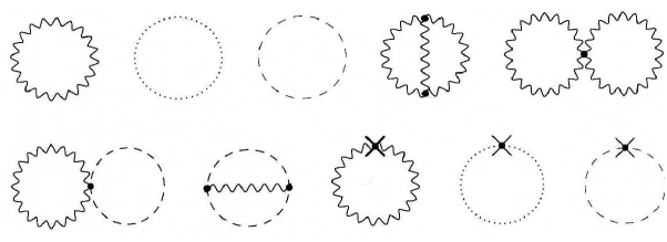
Figure 1: Diagrams, contributing to the two-loop $\beta$-function of the $N=1$ supersymmetric Yang–Mills theory.

With the higher derivative regularization the propagator of the quantum field is

$$\frac{1}{q^{2}(1+q^{2n}/\Lambda^{2n})}$$ (71)

(in the Euclidean space after the Weak rotation). Feynman rules for vertexes, containing two lines of the quantum field $V$, are also changed. In particular, the vertex with a single line of the background superfield ${\bf V}$, which has the momentum $p$, (it is denoted by a bold wavy line) is

(72)

and the vertex with two lines of the background superfield ${\bf V}$, which have momentums $p$ and $-p$, is

$$+{\bf V}^{2}((k+p)^{2}-k^{2})^{2}\Big{)}\Bigg{(}\frac{(k+p)^{2n+2}-k^{2n+2}}{((k+p)^{2}-k^{2})^{2}}-\frac{(n+1)k^{2n}}{(k+p)^{2}-k^{2}}\Bigg{)}-4{\bf V}\partial^{2}\Pi_{1/2}{\bf V}.\qquad$$ (73)

According to the calculations, the two-loop contribution of the Faddeev–Popov ghosts to the Gell-Mann–Low function is 0 that agrees, for example, with Ref. [39]. (Integrals, defining the two-point Green function, appeared to be some finite constants for the ghosts.)

As we already mentioned, the total two-loop contribution of the two-point diagrams to the effective action can be presented in form (38) due to the Slavnov–Taylor identity. To find the function $d^{-1}$ up to an unessential constant, we differentiate it with respect to $\ln\Lambda$, and then set the external momentum $p$ to 0. Later we will see that the result is a finite constant $d_{1}$:

$$\frac{d}{d\ln\Lambda}d^{-1}(\alpha,\Lambda/p)\Bigg{|}_{p=0}=d_{1}.$$ (74)

Therefore, the function $d^{-1}$ depends on the momentum logarithmically

$$d^{-1}(\alpha,\Lambda/p)=d_{1}\ln\frac{\Lambda}{p}+\mbox{const}.$$ (75)

Calculating explicitly two-loop diagrams, presented in Fig. 1 (so far without diagrams with counterterm insertions), differentiating the result with respect to $\ln\Lambda$, and, then, setting $p=0$, we obtain (in the Euclidean space, after the Weak rotation)

$$d_{1}=8\pi\cdot 6\pi\,\alpha_{0}\,\int\frac{d^{4}k}{(2\pi)^{4}}\frac{1}{k^{2}}\frac{d}{dk^{2}}\frac{d}{d\ln\Lambda}\int\frac{d^{4}q}{(2\pi)^{4}}\Big{(}q^{2}(1+q^{2n}/\Lambda^{2n})\Big{)}^{-1}\Bigg{\{}\Big{(}(q+k)^{2}\times$$

$$\times(1+(q+k)^{2n}/\Lambda^{2n})\Big{)}^{-1}\Bigg{[}2(n+1)\Big{(}1+k^{2n}/\Lambda^{2n}\Big{)}^{-1}-2n\Big{(}1+k^{2n}/\Lambda^{2n}\Big{)}^{-2}\Bigg{]}\Bigg{\}}.$$ (76)

It is important to note that taking the limit $p\to 0$ is rather nontrivial, because the final result can contain infrared divergent terms, proportional to $p$ or $p^{2}$, or terms, proportional to $p$, but giving a finite contribution to $d_{1}$. However, the calculation shows that all such terms are cancelled. Moreover, the sum of diagrams appeared to be a total derivative with respect to the module of the loop momentum, so that the integral with respect to $d^{4}k$, which is contained in Eq. (3.2), can be easily calculated by Eq. (60). All substitutions at the upper limit are 0 due to the higher derivative regularization, and only the substitution at the lower limit is nonzero. Using equations, presented above, we obtain

$$d_{1}=-6\alpha_{0}\frac{d}{d\ln\Lambda}\int\frac{d^{4}q}{(2\pi)^{4}}\Big{(}q^{2}(1+q^{2n}/\Lambda^{2n})\Big{)}^{-2}.$$ (77)

This integral can be also easily calculated in the four-dimensional spherical coordinates:

$$d_{1}=\frac{12\alpha_{0}}{\pi}\int\frac{d^{4}q}{(2\pi)^{4}}\frac{1}{q^{4}}q^{2}\frac{d}{dq^{2}}(1+q^{2n}/\Lambda^{2n})^{-2}=\frac{3\alpha_{0}}{4\pi^{3}}(1+q^{2n}/\Lambda^{2n})^{-2}\Bigg{|}_{0}^{\infty}=-\frac{3\alpha_{0}}{4\pi^{2}}.$$ (78)

(We note that the result does not depend on the regularization parameter $n$.) Therefore, in the two-loop approximation

$$d_{0}^{-1}(\alpha_{0},\Lambda/p)=\frac{1}{\alpha_{0}}-\frac{3C_{2}}{2\pi}\ln\frac{\Lambda}{p}-\frac{3\alpha_{0}C_{2}^{2}}{(2\pi)^{2}}\ln\frac{\Lambda}{p}+O(\alpha_{0}^{2}),$$ (79)

where $d_{0}$ denotes the function $d$, calculated without diagrams with counterterms insertions.

Therefore, the Gell-Mann–Low function, defined by Eq. (39), in the two-loop approximation is

$$\beta(\alpha)=-\frac{3C_{2}\alpha^{2}}{2\pi}-\frac{3\alpha^{3}C_{2}^{2}}{(2\pi)^{2}}+O(\alpha^{4})$$ (80)

and coincides with the expansion of the exact NSVZ $\beta$-function in the considered order. We note that this result does not depend on a possible finite constant in Eq. (79).

For calculating quantum corrections it is also necessary to take into account diagrams with counterterms insertions. Usually, adding counterterms is equivalent to splitting the bare coupling constant into the renormalized coupling constant and some infinite additional term. However, using noninvariant regularizations (and, in particular, the regularization, breaking the BRST-invariance, which is used here), it is also necessary to add counterterms, restoring the Slavnov–Taylor identities [25, 26] in each order of the perturbation theory. In general, it is necessary to analyze such counterterms. However, in the considered case the situation is simpler. Really, the one-loop two-point Green function for the Faddeev–Popov ghosts is finite and does not depend on regularization. Interaction of ghosts with the background field is fixed by the background gauge invariance, which is unbroken with the considered regularization. Therefore, additional counterterms do not contribute to subtraction diagrams, containing a loop of the Faddeev–Popov ghosts, in the two-loop approximation. Moreover, terms with the Faddeev–Popov ghosts do not evidently depend on whether the bare or renormalized coupling constant is in the gauge fixing action. Hence, their contributions do not also depend on a way of splitting the bare coupling constant into the renormalized one and counterterms.

Quantizing the theory we also write the bare coupling constant $e_{0}$ in the gauge fixing terms. Therefore, a part of the action, quadratic in the quantum field, is written as

$$\frac{1}{2e_{0}^{2}}\mbox{tr}\,\mbox{Re}\int d^{4}x\,d^{4}\theta\,V\Big{[}\mbox{\boldmath$D$}_{\mu}^{2}\Big{(}1+\frac{\mbox{\boldmath$D$}_{\mu}^{2n}}{\Lambda^{2n}}\Big{)}+2W^{a}\mbox{\boldmath$D$}_{a}\Big{]}V.$$ (81)

Breaking the invariance under the BRST-transformations can lead to the necessity of adding counterterms proportional to

$$\mbox{tr}\int d^{4}x\,d^{4}\theta V\mbox{\boldmath$D$}_{\mu}^{2}V.$$ (82)

(If the background field is 0, this follows from Refs. [27, 28]. Terms, containing the background field, can be restored from the background gauge invariance.) But this means that all one-loop diagrams, including diagrams with insertions of both the counterterms, appearing due to the renormalization of the coupling constant, and the additional counterterms, with a loop of the quantum field $V$, are 0, because they can contain no more than 2 spinor derivatives.

At last, let us consider diagrams, containing a loop of the Nielsen–Kallosh ghosts. Since the Nielsen–Kallosh ghosts exist only in the one-loop approximation, there are no additional counterterms, caused by the noninvariance of the regularization under the BRST-transformations, in these diagrams. However, the contribution of the counterterm diagrams is essential due to the renormalization of the coupling constant. Really, the coefficient in the action for the Nielsen–Kallosh ghosts should be the same as in the gauge fixing terms. Therefore, it must contain the bare coupling constant:

$$\frac{1}{4e_{0}^{2}}\mbox{tr}\int d^{8}x\,B^{+}e^{2{\bf V}}B.$$ (83)

To regularize diagrams with counterterm insertions and a loop of Nielsen–Kallosh ghosts, the action for the corresponding Pauli–Villars fields should be written as

$$\mbox{tr}\int d^{4}x\,\Big{(}\frac{1}{4e_{0}^{2}}\int d^{4}\theta\,B_{PV}^{+}e^{2{\bf V}}B_{PV}+\frac{M_{B}}{2e^{2}}\int d^{2}\theta B_{PV}^{2}+\frac{M_{B}}{2e^{2}}\int d^{2}\theta(B_{PV}^{+})^{2}\Big{)}.$$ (84)

This expression also contains the bare coupling constant $e_{0}$. $M_{B}$ is proportional to the regularization parameter $\Lambda$. Really, let us present a bare coupling constant as

$$\frac{1}{e_{0}^{2}}=\frac{1}{e^{2}}Z_{3},$$ (85)

where $e$ is the renormalized coupling constant, and $Z_{3}$ is the renormalization constant. Then, expanding the Pauli–Villars determinant for the Nielsen–Kallosh ghosts in powers of $Z_{3}-1$, we obtain terms, regularizing diagrams with insertions of counterterms.

However, due to inserting this determinant the generating functional starts to depend on the normalization point at a fixed bare coupling constant $e_{0}$, because the renormalized coupling constant $e$ depends on $\mu$.

In the Abelian case calculating divergences for the action, similar to (84), was made, for example, in Ref. [34]. In the considered case it is also necessary to take into account a factor $-C_{2}/2$, which appears because the Nielsen–Kallosh ghosts are in the adjoint representation of a gauge group and anticommute. (There is only one matter superfield now, instead of 2 matter superfields in the Abelian case.) Moreover, the renormalization constant of a matter field $Z$ should be substituted for the constant $Z_{3}$. Taking into account these comments, the result of Ref. [34] can be formulated as follows. Contribution of the counterterm diagrams for the Nielsen–Kallosh ghosts to $1/\alpha$ can be written as

$$\frac{C_{2}}{2\pi}\ln Z_{3}.$$ (86)

To find this contribution in the two-loop approximation, we note that after the one-loop renormalization the renormalization constant will be

$$Z_{3}=1+\frac{3C_{2}\alpha}{2\pi}\ln\frac{\Lambda}{\mu}+O(\alpha^{2}).$$ (87)

Therefore, the contribution of diagrams with counterterm insertions in the two-loop approximation is written as

$$\frac{3\alpha C_{2}^{2}}{(2\pi)^{2}}\ln\frac{\Lambda}{\mu}.$$ (88)

This contribution exactly cancels the two-loop divergence, so that after the one-loop renormalization

$$d^{-1}(\alpha,\mu/p)=\frac{1}{\alpha}-\frac{3C_{2}}{2\pi}\ln\frac{\mu}{p}-\frac{3\alpha C_{2}^{2}}{(2\pi)^{2}}\ln\frac{\mu}{p}+O(\alpha^{2}).$$ (89)

For an arbitrary order of the perturbation theory it is reasonable to propose that the two-point Green function of the gauge field is given by

$$\frac{1}{d(\alpha,\mu/p)}=\frac{1}{\alpha_{0}}-\frac{1}{2\pi}C_{2}\ln d(\alpha_{0},\Lambda/p)+\frac{1}{2\pi}C_{2}\ln Z_{3}(\alpha,\Lambda/\mu)-\frac{3}{2\pi}C_{2}\ln\frac{\Lambda}{p}.$$ (90)

Really, it is easy to see that the exact NSVZ $\beta$-function is obtained by differentiating this equality with respect to $\ln p$, and the term, proportional to $\ln Z_{3}$ is obtained from contributions of diagrams with counterterms insertions. In the two-loop approximation this equation agrees with (79), if the contribution of diagrams with counterterm insertions is taken into account.

If Eq. (90) is true, then divergences exist only in the one-loop approximation. Really, because

$$\frac{1}{d(\alpha,\mu/p)}=\frac{1}{d(\alpha_{0}(\alpha,\Lambda/\mu),\Lambda/p)}Z_{3}(\alpha,\Lambda/\mu)$$ (91)

is finite, it is necessary to cancel only the one-loop divergence. For this purpose the bare coupling constant is presented as

$$\frac{1}{\alpha_{0}}=\frac{1}{\alpha}+\frac{3}{2\pi}C_{2}\ln\frac{\Lambda}{\mu}.$$ (92)

We note that presence of divergences only in the one-loop approximation in this case does not mean that the physical $\beta$-function has only the one-loop contribution. Really, the physical $\beta$-function is a derivative of the two-point Green function with respect to the logarithm of the momentum if proper boundary conditions are imposed. Such function, as we already saw, has corrections in all loops. A relation between the divergences and the physical $\beta$-function is broken due to the way of the regularization of diagrams with the counterterm insertions, which leads to the dependence of the generating functional on a normalization point at a fixed bare coupling constant [35]. Thus, similar to the electrodynamics, we obtain that the renormalized effective action is exhausted at the one-loop, while the Gell-Mann–Low function has corrections in orders of the perturbation theory. Note, that this conclusion agrees with Ref. [40], in which the two-loop $\beta$-function for the $N=1$ supersymmetric Yang–Mills theory was calculated with the differential renormalization [41].

So, if Eq. (90) is valid, the Gell-Mann–Low function coincides with the exact NSVZ $\beta$-function, and divergences in the two-point Green function exist only in the one-loop approximation.

4 Schwinger–Dyson equations and Slavnov–Taylor identities

4.1 Schwinger–Dyson equations for the contribution of matter superfields

The calculations, described in the previous section, reveal some interesting features of the quantum correction structure, which appear if the higher derivatives are used for regularization. In order to partially explain these features, it is possible to use a method [42, 43], based on substituting solutions of the Slavnov–Taylor identities into the Schwinger–Dyson equations. Here we will discuss only structure of the matter superfields contribution to the exact $\beta$-function. Contribution of diagrams with loops of the gauge fields and ghosts is not so far calculated using this approach.

In order to construct the Schwinger-Dyson equations for model (2) it is necessary to split the action into three parts: the action for the background field, the kinetic term for quantum fields, which does not contain the background field, and interaction, in which the other terms are included:

$$S=S({\bf V})+S_{2}(V,\phi)+S_{I}(V,{\bf V},\phi).$$ (93)

(Earlier we saw that terms of the first order in the superfield $V$, which were obtained from the expansion of the classical action, can be omitted.) So, generating functional (2) can be written as

$$Z[J,j,{\bf V}]=\int d\mu\,\exp\Big{(}iS[{\bf V}]+iS_{2}[V,\phi]+iS_{I}[V,{\bf V},\phi]+iS_{S}+i\int d^{8}x\,JV\Big{)}=$$ (94)

$$=\exp\Big{(}iS[{\bf V}]+iS_{I}\Big{[}\frac{1}{i}\frac{\delta}{\delta J},\frac{1}{i}\frac{\delta}{\delta{\bf J}},\frac{1}{i}\frac{\delta}{\delta j}\Big{]}\Big{)}\times$$

$$\qquad\qquad\qquad\qquad\times\int d\mu\,\exp\Big{(}iS_{2}[V,\phi]+iS_{S}+i\int d^{8}x\,JV+i\int d^{8}x\,{\bf J}{\bf V}\Big{)}\Bigg{|}_{{\bf J}=0},\qquad$$

where ${\displaystyle\int d^{8}x\equiv\int d^{4}x\,d^{4}\theta_{x}}$. Let us differentiate this expression with respect to the background field

$$\frac{\delta}{\delta{\bf V}_{x}}Z[J,j,{\bf V}]=i\frac{\delta S[{\bf V}]}{\delta{\bf V}}\,Z+\exp\Big{(}iS_{I}\Big{[}\frac{1}{i}\frac{\delta}{\delta J},\frac{1}{i}\frac{\delta}{\delta{\bf J}},\frac{1}{i}\frac{\delta}{\delta j}\Big{]}\Big{)}i{\bf J_{x}}\times$$

$$\qquad\qquad\qquad\times\int d\mu\,\exp\Big{(}iS_{2}[V,\phi]+iS_{S}+i\int d^{8}x\,JV+i\int d^{8}x\,{\bf J}{\bf V}\Big{)}\Bigg{|}_{{\bf J}=0}.\qquad$$ (95)

Moving the current ${\bf J}_{x}$ to the left and dividing the result to $Z$, we obtain

$$\frac{\delta}{\delta{\bf V}_{x}}W[J,j,{\bf V}]=\frac{\delta S[{\bf V}]}{\delta{\bf V}_{x}}+\frac{\delta}{\delta{\bf V}_{x}}S_{I}\Big{[}{\bf V},V+\frac{1}{i}\frac{\delta}{\delta J},\phi+\frac{1}{i}\frac{\delta}{\delta j}\Big{]}.$$ (96)

Because the background field ${\bf V}$ is a parameter of the effective action, these equality can be equivalently written as

$$\frac{\delta\Gamma}{\delta{\bf V}_{x}}=\frac{\delta S[{\bf V}]}{\delta{\bf V}_{x}}+\Big{\langle}\frac{\delta}{\delta{\bf V}_{x}}S_{I}\Big{[}{\bf V},V,\phi\Big{]}\Big{\rangle},$$ (97)

where the angular brackets denote taking an expectation value by the ordinary functional integration. Certainly, it is necessary to set the field $V$ (an argument of the effective action) to 0 in the final result.

Let us find a contribution to this expression given by the matter superfields. The corresponding interaction terms are

$$S_{I}=\frac{1}{4}\int d^{8}x\,\phi^{+}\Big{(}e^{\bf V}e^{2V}e^{\bf V}-1\Big{)}\phi+\mbox{similar terms with }\tilde{\phi}.$$ (98)

Differentiating $S_{I}$ with respect to the background field, we obtain that the corresponding contribution to the effective action is written in the form

$$\frac{\delta\Gamma}{\delta{\bf V}_{x}^{a}}=\mbox{Terms without matter}+\sum\limits_{i}c_{i}\frac{\delta}{\delta{\bf V}_{x}^{a}}\Big{\langle}\ln\det PV\Big{(}V,{\bf V},M_{i}\Big{)}\Big{\rangle}+\qquad$$

$$+\frac{1}{4}\frac{\delta}{\delta{\bf V}_{x}^{a}}\int d^{8}x\,\Big{\langle}\phi_{x}^{+}e^{{\bf V}_{x}}e^{2V_{x}}e^{{\bf V}_{x}}\phi_{x}+\mbox{similar terms with }\tilde{\phi}\Big{\rangle}.\quad$$ (99)

We are interested in the two-point Green function of the gauge field, corresponding to the expansion of the effective action in powers of the background field up to the second order terms. This function is evidently symmetric with respect to the indexes, numerating generators of the gauge group. Then, using the form of action for additional sources (2), we easily obtain

$$\frac{1}{4}\Big{\langle}\phi_{x}^{+}T^{a}e^{{\bf V}_{x}}e^{2V_{x}}e^{{\bf V}_{x}}\phi_{x}+\phi_{x}^{+}e^{{\bf V}_{x}}e^{2V_{x}}e^{{\bf V}_{x}}T^{a}\phi_{x}\Big{\rangle}=\frac{1}{i}\mbox{tr}\Bigg{[}T^{a}\Bigg{(}\frac{\delta^{2}\Gamma}{\delta j_{x}^{+}\delta\phi_{0x}^{+}}+\frac{\delta^{2}\Gamma}{\delta j_{x}\delta\phi_{0x}}\Bigg{)}\Bigg{]}.$$ (100)

(Here the derivatives with respect to the sources must be expressed in terms of fields.)

Therefore, using Eq. (4.1) and taking into account similar terms with the fields $\tilde{\phi}$, the corresponding contribution to the two-point Green function of the matter superfield can be written as

$$\frac{\delta\Gamma}{\delta{\bf V}^{b}_{y}\delta{\bf V}^{a}_{x}}=\ldots+e\,\frac{\delta}{\delta{\bf V}^{b}_{y}}\mbox{tr}\Bigg{[}T^{a}\frac{1}{i}\frac{\delta^{2}\Gamma}{\delta j_{x}^{+}\,\delta\phi_{0x}^{+}}-(T^{a})^{t}\frac{1}{i}\frac{\delta^{2}\Gamma}{\delta\tilde{j}_{x}^{+}\,\delta\tilde{\phi}_{0x}^{+}}+\mbox{h.c.}\Bigg{]},$$ (101)

where dots denote contributions of the gauge fields, ghosts, and also all possible Pauli-Villars fields. We note that the calculation of the Pauli-Villars fields contributions are made completely similar to the calculation of ordinary fields contributions [42], and details of this calculation are not presented here. The result will be given below.

Performing differentiation in Eq. (101), this equation can be graphically presented as a sum of two effective diagrams

(102)

The double lines correspond to the effective propagators, which are written as

$$\Bigg{(}\frac{\delta^{2}\Gamma}{\delta\phi_{x}^{+}\delta\phi_{y}}\Bigg{)}^{-1}=-\frac{GD_{x}^{2}\bar{D}_{x}^{2}}{4(\partial^{2}G^{2}+m^{2}J^{2})}\delta^{8}_{xy};\qquad\Bigg{(}\frac{\delta^{2}\Gamma}{\delta\phi_{x}\delta\tilde{\phi}_{y}}\Bigg{)}^{-1}=-\frac{mJ\bar{D}_{x}^{2}}{\partial^{2}G^{2}+m^{2}J^{2}}\delta^{8}_{xy},$$ (103)

depending on the chirality of the ends. The functions $G$ and $J$ are determined by the two-point Green functions of the matter superfield as

$$\frac{\delta^{2}\Gamma}{\delta\phi_{x}^{+}\delta\phi_{y}}=\frac{D_{x}^{2}\bar{D}_{x}^{2}}{16}G(\partial^{2})\delta^{8}_{xy};\qquad\frac{\delta^{2}\Gamma}{\delta\phi_{x}\delta\tilde{\phi}_{y}}=-\frac{\bar{D}_{x}^{2}}{4}mJ(\partial^{2})\delta^{8}_{xy},$$ (104)

where $\delta^{8}_{xy}\equiv\delta^{4}(x-y)\delta^{4}(\theta_{x}-\theta_{y})$.

4.2 Slavnov–Taylor identities and their solutions

The vertex functions in Eq. (102) can be obtained from the Slavnov-Taylor identities. Certainly, it is necessary to take into account that we consider vertex functions, which have an external line of the background field. As we already mentioned above, the effective action is invariant under the background gauge transformations. It is easy to see that this invariance can be expressed by the equality

$$0=\int d^{8}y\,\Bigg{(}\frac{\delta\Gamma}{\delta{\bf V}_{y}^{a}}\delta{\bf V}_{y}^{a}+\frac{\delta\Gamma}{\delta\phi_{y}}\frac{D^{2}}{8\partial^{2}}\delta\phi_{y}+\delta\phi_{y}^{+}\frac{\bar{D}^{2}}{8\partial^{2}}\frac{\delta\Gamma}{\delta\phi_{y}^{+}}+\frac{\delta\Gamma}{\delta\phi_{0y}}\delta\phi_{0y}+\delta\phi_{0y}^{+}\frac{\delta\Gamma}{\delta\phi_{0y}^{+}}+\qquad$$

$$+\mbox{similar terms with $\tilde{\phi}$ and $\tilde{\phi}_{0}$}\Bigg{)},$$ (105)

where

$$\delta\phi_{x}=\Lambda_{x}\phi_{x};\qquad\delta\phi_{x}^{+}=\phi_{x}^{+}\Lambda_{x}^{+};\qquad\delta\phi_{0x}=\Lambda_{x}\phi_{0x};\qquad\delta\phi_{0x}^{+}=\phi_{0x}^{+}\Lambda_{x}^{+};$$

$$\delta{\bf V}_{x}=-\frac{1}{2}\Big{(}\Lambda_{x}+\Lambda_{x}^{+}\Big{)}+O({\bf V}).$$ (106)

Here $\Lambda$ is an arbitrary chiral superfield, and all other terms in $\delta{\bf V}$ are proportional at least to the first degree of the background field. (For the fields $\tilde{\phi}$ e.t.c. the transformation laws can be also easily written.) Let us differentiate Eq. (4.2) with respect to $\Lambda_{y}^{a}$, $\phi^{+}_{0z}$, $\phi_{x}$ or with respect to $\Lambda_{y}^{a}$, $\tilde{\phi}_{0z}$, $\phi_{x}$. As a result we obtain the Slavnov-Taylor identities

$$0=\frac{1}{2e}(\bar{D}_{y}^{2}+D_{y}^{2})\frac{\delta\Gamma}{\delta{\bf V}_{y}^{a}\delta\phi^{+}_{0z}\delta\phi_{x}}-\frac{\delta\Gamma}{\delta\phi_{0z}^{+}\delta\phi_{y}}T^{a}\bar{D}_{y}^{2}\delta^{8}_{xy}-D_{y}^{2}\Big{(}\delta^{8}_{yz}T^{a}\frac{\delta\Gamma}{\delta\phi_{0y}^{+}\delta\phi_{x}}\Big{)};$$

$$0=\frac{1}{2e}(\bar{D}_{y}^{2}+\bar{D}_{y}^{2})\frac{\delta^{3}\Gamma}{\delta{\bf V}^{a}_{y}\delta\tilde{\phi}_{0z}\delta\phi_{x}}-\frac{\delta^{2}\Gamma}{\delta\tilde{\phi}_{0z}\delta\phi_{y}}T^{a}\bar{D}_{y}^{2}\delta^{8}_{xy}+\bar{D}_{y}^{2}\Big{(}\delta^{8}_{yz}T^{a}\frac{\delta^{2}\Gamma}{\delta\tilde{\phi}_{0y}\delta\phi_{x}}\Big{)},\qquad$$ (107)

where

$$\frac{\delta^{2}\Gamma}{\delta\phi_{y}\delta\phi_{0z}^{+}}=-\frac{1}{8}G(\partial^{2})\bar{D}_{y}^{2}\delta^{8}_{yz};\qquad\frac{\delta^{2}\Gamma}{\delta\tilde{\phi}_{y}^{*}\delta\phi_{0z}^{+}}=\frac{m}{32\partial^{2}}\Big{(}J(\partial^{2})-1\Big{)}D_{y}^{2}\bar{D}_{y}^{2}\delta^{8}_{yz}.$$ (108)

Solutions of Eqs. (4.2) are the functions

$$\frac{\delta^{3}\Gamma}{\delta{\bf V}^{a}_{y}\delta\phi^{+}_{0z}\delta\phi_{x}}\Bigg{|}_{p=0}=e\Bigg{[}-2\partial^{2}\Pi_{1/2}{}_{y}\Big{(}\bar{D}_{y}^{2}\delta^{8}_{xy}\delta^{8}_{yz}\Big{)}F(q^{2})+\frac{1}{8}D^{b}C_{bc}\bar{D}_{y}^{2}\Big{(}\bar{D}_{y}^{2}\delta^{8}_{xy}D_{y}^{c}\delta^{8}_{yz}\Big{)}f(q^{2})-\vphantom{\frac{1}{2}}$$

$$-\frac{1}{16}q^{\mu}G^{\prime}(q^{2})\bar{D}\gamma^{\mu}\gamma_{5}D_{y}\Big{(}\bar{D}_{y}^{2}\delta^{8}_{xy}\delta^{8}_{yz}\Big{)}-\frac{1}{4}\bar{D}_{y}^{2}\delta^{8}_{xy}\delta^{8}_{yz}\,G(q^{2})\Bigg{]}T^{a};$$ (109)

$$\frac{\delta^{3}\Gamma}{\delta{\bf V}^{a}_{y}\delta\tilde{\phi}_{0z}\delta\phi_{x}}\Bigg{|}_{p=0}=e\Bigg{[}\,\frac{m}{32}D^{b}C_{bc}D_{y}^{2}\Big{(}D_{y}^{2}\bar{D}_{y}^{2}\delta^{8}_{xy}D_{y}^{c}\delta^{8}_{yz}\Big{)}h(q^{2})+\frac{m}{16}J^{\prime}(q^{2})\Bigg{(}\bar{D}_{y}^{2}\delta^{8}_{xy}D_{y}^{2}\delta^{8}_{yz}-$$

$$-D_{y}^{2}\bar{D}_{y}^{2}\delta^{8}_{xy}\delta^{8}_{yz}\Bigg{)}+\frac{m}{16}\Bigg{(}\frac{J^{\prime}(q^{2})}{q^{2}}-\frac{J(q^{2})-1}{q^{4}}\Bigg{)}\Bigg{(}D_{y}^{2}\bar{D}_{y}^{2}\delta^{8}_{xy}\frac{\bar{D}_{y}^{2}D_{y}^{2}}{16}\delta^{8}_{yz}+D_{y}^{2}\bar{D}_{y}^{2}\delta^{8}_{xy}q^{2}\delta^{8}_{yz}\Bigg{)}\Bigg{]}T^{a}.$$

Here the primes denote derivatives with respect to $q^{2}$,

$$\Pi_{1/2}=-\frac{1}{8\partial^{2}}D^{a}\bar{D}^{2}D_{a}=-\frac{1}{8\partial^{2}}\bar{D}^{a}D^{2}\bar{D}_{a}$$ (111)

is a supersymmetric transverse projection operator, and the functions $F$, $f$ and $h$ can not be determined from the Slavnov-Taylor identities.

Functions (4.2) and (4.2) allow finding ordinary Green functions by the identities

$$-\frac{D_{z}^{2}}{2}\frac{\delta^{3}\Gamma}{\delta{\bf V}^{a}_{x}\delta\phi_{y}\delta\phi^{+}_{0z}}=\frac{\delta^{3}\Gamma}{\delta{\bf V}^{a}_{x}\delta\phi_{y}\delta\phi^{+}_{z}};\qquad-\frac{\bar{D}_{z}^{2}}{2}\frac{\delta^{3}\Gamma}{\delta{\bf V}^{a}_{x}\delta\phi_{y}\delta\tilde{\phi}_{0z}}=\frac{\delta^{3}\Gamma}{\delta{\bf V}^{a}_{x}\delta\phi_{y}\delta\tilde{\phi}_{z}}.$$ (112)

We note that the additional sources in Eq. (2) were specially introduced in order that such identities take place. Using Eqs. (112) we find

$$\frac{\delta^{3}\Gamma}{\delta{\bf V}^{a}_{y}\delta\phi^{+}_{z}\delta\phi_{x}}\Bigg{|}_{p=0}=e\Bigg{[}\partial^{2}\Pi_{1/2}{}_{y}\Big{(}\bar{D}_{y}^{2}\delta^{8}_{xy}D_{y}^{2}\delta^{8}_{yz}\Big{)}F(q^{2})+$$

$$\qquad\qquad+\frac{1}{32}q^{\mu}G^{\prime}(q^{2})\bar{D}\gamma^{\mu}\gamma_{5}D_{y}\Big{(}\bar{D}_{y}^{2}\delta^{8}_{xy}D_{y}^{2}\delta^{8}_{yz}\Big{)}+\frac{1}{8}\bar{D}_{y}^{2}\delta^{8}_{xy}D_{y}^{2}\delta^{8}_{yz}\,G(q^{2})\Bigg{]}T^{a};$$ (113)

$$\frac{\delta^{3}\Gamma}{\delta{\bf V}^{a}_{y}\delta\tilde{\phi}_{z}\delta\phi_{x}}\Bigg{|}_{p=0}=-\frac{em}{32}J^{\prime}(q^{2})\Bigg{[}\bar{D}_{y}^{2}\delta^{8}_{xy}D_{y}^{2}\bar{D}_{y}^{2}\delta^{8}_{yz}-D_{y}^{2}\bar{D}_{y}^{2}\delta^{8}_{xy}\bar{D}_{y}^{2}\delta^{8}_{yz}\Bigg{]}T^{a}.\qquad$$ (114)

4.3 Exact Gell-Mann–Low function.

We will calculate

$$\frac{d}{d\ln\Lambda}\frac{\delta\Gamma}{\delta{\bf V}^{b}_{y}\delta{\bf V}^{a}_{x}}\Bigg{|}_{p=0}.$$ (115)

Note that the regularization by higher covariant derivatives is essentially used here, because it allows differentiating the integrand and taking the limit of zero external momentum.

After substituting the vertex functions from Eqs. (4.2), (114), (4.2), (4.2) and the propagators from Eqs. (103), the Weak rotation, and some simple transformations, using the algebra of the covariant derivatives, we obtain that in the momentum representation the first diagram is written as

$$-C(R)\frac{d}{d\ln\Lambda}\mbox{tr}\int\frac{d^{4}p}{(2\pi)^{4}}\frac{d^{4}q}{(2\pi)^{4}}\Bigg{\{}{\bf V}\partial^{2}\Pi_{1/2}{\bf V}\Bigg{[}\frac{8GF}{q^{2}G^{2}+m^{2}J^{2}}-\frac{m^{2}JJ^{\prime}}{2q^{2}(q^{2}G^{2}+m^{2}J^{2})}+$$

$$+\frac{1}{2}\frac{d}{dq^{2}}\Bigg{(}\ln\Big{(}q^{2}G^{2}+m^{2}J^{2}\Big{)}+\frac{m^{2}J}{q^{2}G^{2}+m^{2}J^{2}}\Bigg{)}\Bigg{]}+{\bf V}^{2}\frac{G^{2}}{q^{2}G^{2}+m^{2}J^{2}}\Bigg{\}},$$ (116)

and the second one is

$$-C(R)\frac{d}{d\ln\Lambda}\mbox{tr}\int\frac{d^{4}p}{(2\pi)^{4}}\frac{d^{4}q}{(2\pi)^{4}}\Bigg{\{}{\bf V}\partial^{2}\Pi_{1/2}{\bf V}\Bigg{[}-\frac{8GF}{q^{2}G^{2}+m^{2}J^{2}}-\frac{m^{2}JJ^{\prime}}{2q^{2}(q^{2}G^{2}+m^{2}J^{2})}+$$ (117)

$$+\frac{m^{2}J(J-1)}{2q^{4}(q^{2}G^{2}+m^{2}J^{2})}-\frac{8Gf+8m^{2}Jh}{q^{2}G^{2}+m^{2}J^{2}}\Bigg{]}-{\bf V}^{2}\frac{G^{2}}{q^{2}G^{2}+m^{2}J^{2}}\Bigg{\}}.$$

Let $d_{0}$ denotes the function $d$, calculated without taking into account counterterm insertions on lines of matter superfields, or, equivalently, at $Z=1$. Moreover, we take into account that for finding the Gell-Mann–Low function it is necessary to set $m=0$. Then, adding the results for the effective diagrams in the Schwinger–Dyson equation and using Eq. (38), we obtain

$$-\frac{1}{16\pi}\frac{d}{d\ln\Lambda}d_{0}^{-1}\Big{|}_{p=0}=\ldots-C(R)\int\frac{d^{4}q}{(2\pi)^{4}}\frac{d}{d\ln\Lambda}\Bigg{\{}\frac{1}{2q^{2}}\frac{d}{dq^{2}}\ln\Big{(}q^{2}G^{2}\Big{)}-\frac{8f}{q^{2}G}-\qquad$$

$$-\sum\limits_{i}c_{i}\frac{1}{2q^{2}}\frac{d}{dq^{2}}\Bigg{(}\ln\Big{(}q^{2}G_{PV}^{2}+M_{i}^{2}J_{PV}^{2}\Big{)}+\frac{M_{i}^{2}J_{PV}}{q^{2}G_{PV}^{2}+M_{i}^{2}J_{PV}^{2}}\Bigg{)}+$$

$$+\sum\limits_{i}c_{i}\Bigg{(}\frac{M_{i}^{2}J_{PV}\,\Big{(}2q^{2}J_{PV}^{\prime}-(J_{PV}-1)\Big{)}}{2q^{4}\Big{(}q^{2}G_{PV}^{2}+M_{i}^{2}J_{PV}^{2}\Big{)}}+\frac{8G_{PV}f_{PV}+8M_{i}^{2}J_{PV}h_{PV}}{q^{2}G_{PV}^{2}+M_{i}^{2}J_{PV}^{2}}\Bigg{)}\Bigg{\}}.\qquad$$ (118)

(The dots denote contributions of the gauge fields and ghosts, and the symbol $PV$ means that the corresponding function is calculated for the Pauli–Villars fields.) We see that all noninvariant terms, proportional to ${\bf V}^{2}$, and terms, containing the unknown function $F$, are completely cancelled. Nevertheless, there are the functions $f$ and $h$, which can not be found from the Ward identities, in the final result.

It is important to note that many contributions in this expression are integrals of total derivatives. This partially explains the feature, noted earlier. However, calculations show that all terms in this expression should be integrals of total derivatives. Moreover, the accurate analysis of the calculation, described above, shows that terms, which are not factorized into total derivatives in Eq. (4.3), are always equal to 0. Therefore, it is possible to suggest the equality

$$\int\frac{d^{4}q}{(2\pi)^{4}}\frac{d}{d\ln\Lambda}\Bigg{(}\frac{m^{2}J\,(2q^{2}J^{\prime}-(J-1))}{2q^{4}(q^{2}G^{2}+m^{2}J^{2})}+\frac{8Gf+8m^{2}Jh}{q^{2}G^{2}+m^{2}J^{2}}\Bigg{)}=0.$$ (119)

For the massless theory it can be written in the simpler form

$$\int\frac{d^{4}q}{(2\pi)^{4}}\frac{d}{d\ln\Lambda}\frac{f}{q^{2}G}=0.$$ (120)

We will call Eqs. (119) and (120) the new identity for the Green functions. It is not a consequence of the gauge symmetry, the supersymmetry, or the superconformal symmetry. Below we will discuss it in more details, and now let us consider its consequences. If the new identity for the Green functions is true, then we obtain

$$\frac{d}{d\ln\Lambda}\,d_{0}^{-1}(\alpha_{0},\Lambda/p)\Bigg{|}_{p=0}=16\pi C(R)\,\int\frac{d^{4}q}{(2\pi)^{4}}\frac{d}{d\ln\Lambda}\frac{1}{2q^{2}}\frac{d}{dq^{2}}\Bigg{\{}\ln(q^{2}G^{2})-\qquad$$

$$-\sum\limits_{i}c_{i}\ln\Big{(}q^{2}G_{PV}^{2}+M_{i}^{2}J_{PV}^{2}\Big{)}-\sum\limits_{i}c_{i}\frac{M_{i}^{2}J_{PV}}{q^{2}G_{PV}^{2}+M_{i}^{2}J_{PV}^{2}}\Bigg{\}}.$$ (121)

The obtained integral is reduced to the total derivative in the four-dimensional spherical coordinates, only the substitution at the low limit being different from 0 [42]:

$$\frac{d}{d\ln\Lambda}\,d_{0}^{-1}\Bigg{|}_{p=0}=-\frac{C(R)}{2\pi}\,\frac{d}{d\ln\Lambda}\Bigg{\{}\ln G(0)^{2}-\sum\limits_{i}c_{i}\ln\Big{(}M_{i}^{2}J_{PV}(0,a_{i})^{2}\Big{)}-\qquad$$

$$-\sum\limits_{i}c_{i}\frac{1}{J_{PV}(0,a_{i})}\Bigg{\}}=\frac{1}{\pi}C(R)\Bigg{(}1-\frac{d\ln G}{d\ln\Lambda}\Bigg{)}\Bigg{|}_{q=0}.$$ (122)

Here we took into account that the function $J_{PV}(q^{2}/\Lambda^{2},a_{i})$ in the limit $q\to 0$ tended to some finite constants, because it was defined by convergent (even in the limit $\Lambda\to\infty$), dimensionless integrals, which did not contain infrared divergences. Because both parts of Eq. (4.3) depend on $\alpha_{0}$ and $\Lambda/p$, it allows finding the expression for $d_{0}^{-1}$ up to an insignificant numerical constant

$$d_{0}^{-1}(\alpha_{0},\Lambda/p)=\frac{1}{\pi}C(R)\Big{(}\ln\frac{\Lambda}{p}-\ln G(\alpha_{0},\Lambda/p)\Big{)}+\mbox{const}.$$ (123)

Now let us calculate the sum of diagrams with counterterm insertions on lines of matter superfields exactly to all orders of the perturbation theory. For this purpose we make the substitution

$$\phi\to\phi/\sqrt{Z};\quad\tilde{\phi}\to\tilde{\phi}/\sqrt{Z};\quad\Phi\to\Phi/\sqrt{Z};\quad\tilde{\Phi}\to\tilde{\Phi}/\sqrt{Z}$$ (124)

in the generating functional. Then, it is easy to see that if $\phi_{0}$ and $j$ are 0, the dependence on the renormalization constant $Z$ can be found by the replacement

$$m\to m/Z;\qquad M_{i}\to M_{i}/Z.$$ (125)

Making this replacement in Eq. (4.3) it is possible to restore the dependence of the effective action on $Z$:

$$d^{-1}(\alpha,\mu/p)=d_{0}^{-1}(\alpha_{0},\Lambda/p)-\frac{C(R)}{\pi}\ln Z(\alpha,\Lambda/\mu)=$$

$$\qquad\qquad\qquad=\frac{1}{\alpha_{0}}+\frac{1}{\pi}C(R)\Big{(}\ln\frac{\Lambda}{p}-\ln ZG(\alpha,\mu/p)\Big{)}+\mbox{const}.\qquad$$ (126)

Differentiating this expression with respect to the momentum $p$, we obtain the Gell-Mann–Low function

$$\beta(d)=\frac{\partial d}{\partial\ln p}=-d^{2}\frac{\partial}{\partial\ln p}\,d^{-1}=\frac{d^{2}}{\pi}C(R)\Big{(}1-\gamma(d)\Big{)}.$$ (127)

This expression corresponds to a contribution of the matter superfields to the exact NSVZ $\beta$-function (1). (It is necessary to take into account that in the considered case the matter fields are in the representation $R+\bar{R}$.) According to Eq. (4.3), to cancel the dependence on $\Lambda$, the bare coupling constant should be presented in the form

$$\frac{1}{\alpha_{0}}=\frac{1}{\alpha}-\frac{1}{\pi}C(R)\ln\frac{\Lambda}{\mu}.$$ (128)

This means that there are divergences only in the one-loop approximation.

Note that if the new identity were not valid [43], the contribution of the matter superfields to the exact $\beta$-function should be modified as follows:

$$\frac{\alpha^{2}C(R)}{\pi}\Big{(}1-\gamma(\alpha)-\lim\limits_{p\to 0}\frac{16p^{2}f}{G}\Big{)}.$$ (129)

5 New identity for Green functions

The new identity for the Green functions in the massive and massless cases are given by Eqs. (119) and (120) respectively. In the both cases it can be equivalently rewritten in the following functional form [43] (for the simplicity we will consider here the Abelian case):

$$\int d^{8}x\,d^{8}y\,{\bf V}_{y}D^{a}{\bf V}_{x}\frac{d}{d\ln\Lambda}\frac{D_{az}\bar{D}_{z}^{2}}{\partial^{2}}\frac{\delta^{3}\Gamma}{\delta j_{z}^{+}\delta{\bf V}_{y}\delta\phi_{0x}^{+}}\Bigg{|}_{z=x,p=0}=0,$$ (130)

where we assume that the derivatives with respect to sources should be expressed through the derivatives with respect to fields. The condition $p=0$ means that in this case the background field ${\bf V}$ depends only on variables $\theta$ and is independent of the usual coordinates $x^{\mu}$. The derivative with respect to $\ln\Lambda$ in this expression is essential. In order to check this, let us consider for simplicity the massless case and suppose that these derivative is absent. Then, from the dimensional considerations

$$\int\frac{d^{4}q}{(2\pi)^{4}}\frac{f}{q^{2}G}=\int\frac{d^{4}q}{(2\pi)^{4}}\frac{a(q^{2}/\Lambda^{2})}{q^{4}},$$ (131)

where $a$ is a dimensionless function, which is rapidly decreasing at $q\to\infty$. In general, it is possible that $a(0)\neq 0$. But if $a(0)\neq 0$, then the integral in Eq. (131) is not well defined: it is divergent in the infrared region. In order to avoid this we introduce the additional differentiation with respect to $\ln\Lambda$. Due to its presence the term $a(0)$, which does not depend on $\Lambda$, disappears, and the integral becomes finite in the infrared region. Thus, without the derivative with respect to $\ln\Lambda$ the left hand side of the new identity is not well defined. It is essential that the differentiation with respect to $\ln\Lambda$ is possible due to using the higher covariant derivative regularization.

To prove equality (130) it is necessary to replace differentiation with respect to the sources by the differentiation with respect to fields and substitute expressions for the vertexes and propagators, presented earlier.

Let us rewrite identity (130) in a different form. We commute the differentiations with respect to ${\bf V}$ and $\phi_{0}$, and again use the Schwinger–Dyson equations, keeping only contributions of the matter superfields as earlier. The result is

$$\int d^{8}x\,d^{8}y\,{\bf V}_{y}D^{a}{\bf V}_{x}\frac{d}{d\ln\Lambda}\frac{D_{az}\bar{D}_{z}^{2}}{\partial^{2}}\frac{\delta^{2}}{\delta j_{z}^{+}\delta\phi_{0x}^{+}}\Big{\langle}(\phi^{+}e^{2V}\phi-\tilde{\phi}^{+}e^{-2V^{t}}\tilde{\phi}+$$

$$+\phi_{0}^{+}e^{2V}\phi-\tilde{\phi}_{0}^{+}e^{-2V^{t}}\tilde{\phi})_{y}\Big{\rangle}\Bigg{|}_{z=x,p=0}=0.$$ (132)

A contribution of terms, containing $\phi_{0}^{+}$ is 0, because after performing the differentiation we obtain

$$\Big{\langle}\frac{D_{a}\bar{D}^{2}}{\partial^{2}}\phi_{x}^{+}e^{2V_{x}}\phi_{x}\Big{\rangle}=\frac{D_{az}\bar{D}_{z}^{2}}{\partial^{2}}\frac{\delta^{2}\Gamma}{\delta j_{z}^{+}\delta\phi_{0x}^{+}}\Bigg{|}_{z=x}=0.$$ (133)

(In order to verify the last equality it is necessary to express the derivative with respect to the source through derivatives with respect to fields, use Eqs. (108) and (103), and take into account that the expression $\hat{P}_{x}\delta^{4}(\theta_{x}-\theta_{y})\Big{|}_{\theta_{x}=\theta_{y}}$ is not 0 only if the operator $\hat{P}$ contains 4 spinor derivatives.

Therefore, the new identity can be written in terms of composite operators correlators as

$$0=\frac{d}{d\ln\Lambda}\Big{\langle}\int d^{8}x\,D^{a}{\bf V}_{x}\Big{(}\frac{D_{a}\bar{D}^{2}}{\partial^{2}}\phi^{+}e^{2V}\phi\Big{)}_{x}\int d^{8}y\,{\bf V}_{y}\Big{(}\phi^{+}e^{2V}\phi-\tilde{\phi}^{+}e^{-2V^{t}}\tilde{\phi}\Big{)}_{y}\Big{\rangle}\Big{|}_{p=0}.$$ (134)

Taking into account the identity

$$\frac{D^{2}\bar{D}^{2}}{\partial^{2}}\phi^{+}=-16\phi^{+}$$ (135)

this expression can be rewritten as

$$0=\frac{d}{d\ln\Lambda}\Big{\langle}\int d^{8}x\,D^{a}{\bf V}_{x}\Big{(}\frac{D_{a}\bar{D}^{2}}{\partial^{2}}\phi^{+}e^{2V}\phi\Big{)}_{x}\times$$

$$\qquad\qquad\qquad\int d^{8}y\,{\bf V}_{y}\Big{(}\frac{D^{2}\bar{D}^{2}}{\partial^{2}}\phi^{+}e^{2V}\phi-\frac{D^{2}\bar{D}^{2}}{\partial^{2}}\tilde{\phi}^{+}e^{-2V^{t}}\tilde{\phi}\Big{)}_{y}\Big{\rangle}\Big{|}_{p=0}.\qquad$$ (136)

Using the Leibnitz rule for the supersymmetric covariant derivative, we find

$$\frac{D^{2}\bar{D}^{2}}{\partial^{2}}({\bf V}\phi^{+})={\bf V}\frac{D^{2}\bar{D}^{2}}{\partial^{2}}\phi^{+}+2D^{a}{\bf V}\frac{D_{a}\bar{D}^{2}}{\partial^{2}}\phi^{+}-8i(\gamma^{\mu}C)_{ab}D^{b}\bar{D}^{a}{\bf V}\frac{\partial_{\mu}}{\partial^{2}}\phi^{+}+\ldots,$$ (137)

where dots denote all terms, which do not contribute to the considered correlator, because the momentum of the field ${\bf V}$ is 0. (As a consequence, all terms, in which more than 4 spinor derivatives act on the fields ${\bf V}$ are 0.) The first term in Eq. (137) also does not contribute to the considered correlator, because (the sources are not set to 0)

$$\frac{d}{d\ln\Lambda}\Big{\langle}\int d^{8}x\,\frac{D^{2}\bar{D}^{2}}{16\partial^{2}}({\bf V}\phi^{+})e^{2V}\phi\Big{\rangle}=\frac{d}{d\ln\Lambda}\Big{\langle}\int d^{8}x\,({\bf V}\phi^{+})\frac{D^{2}\bar{D}^{2}}{16\partial^{2}}(e^{2V}\phi)\Big{\rangle}=\qquad$$

$$=\frac{d}{d\ln\Lambda}\int d^{8}x\,\frac{\delta}{\delta j_{x}^{+}}\frac{D^{2}\bar{D}^{2}}{4\partial^{2}}\frac{\delta\Gamma}{\delta\phi_{0x}^{+}}=-\frac{d}{d\ln\Lambda}\int d^{8}x\,\frac{\delta}{\delta j_{x}^{+}}\frac{D^{2}}{2\partial^{2}}\frac{\delta\Gamma}{\delta\phi_{x}^{+}}=0.$$ (138)

Therefore, the new identity can be equivalently written as

$$\frac{d}{d\ln\Lambda}\Big{\langle}\int d^{8}x\,D^{a}{\bf V}_{x}\frac{D_{a}\bar{D}^{2}}{\partial^{2}}\phi_{x}^{+}e^{2V_{x}}\phi_{x}\int d^{8}y\,\Big{(}\Big{[}D^{b}{\bf V}_{y}\frac{D_{b}\bar{D}^{2}}{\partial^{2}}\phi_{y}^{+}-4i(\gamma^{\mu}C)_{bc}\times$$

$$\times D^{c}\bar{D}^{b}{\bf V}_{y}\frac{\partial_{\mu}}{\partial^{2}}\phi_{y}^{+}\Big{]}e^{2V_{y}}\phi_{y}-\mbox{similar terms with $\tilde{\phi}$}\Big{)}\Big{\rangle}\Big{|}_{p=0}=0.\qquad$$ (139)

Actually this equality has been already written in Ref. [44] on the language of Feynman diagrams. Nevertheless, its strict functional formulation is first presented here.

6 Verification of new identity for Green functions

6.1 Four-loop approximation in the Abelian case

In order to be sure that the calculations, presented above, and the proposal about existence of the new identity for Green functions are true, it is necessary to perform a verification by explicit calculations. Making this verification is considerably simplified, if we note that expressions (4.3) and (117) allow not only finding sums of all diagrams with two external lines of the gauge field, but also summing special classes of such diagrams. Such classes of diagrams are obtained from a frame, to which external lines are attached by all possible ways. In particular, in order to verify Eqs. (4.3) and (117) in Ref. [45] we considered a group of diagrams, which were obtained from a frame, presented in Fig. 2, by attaching two external line of the gauge field.

Figure 2: Schematic picture of group of diagrams, which is used for verification of new identity

This diagrams can be calculated by two different ways:

1. using Eqs. (4.3) and (117) and the functions $G$, $f$ and $F$, obtained preliminary.

2. by explicit calculation using supergraphs.

Thus it is possible to perform a four-loop verification of Eqs. (4.3) and (117), and also identity (120).

In order to find diagrams which will be essential for obtaining the unknown functions $G$, $f$ and $F$ in the considered case, it is convenient to use the following simple speculations: A diagram, presented in Fig. 2, can be considered as a formal product of the one- and two-loop diagrams with $\phi^{*}$ and $\phi$ external lines (pairs of their ends are identified):

or as the three-loop diagrams with the identified ends:

The parts of the diagram, obtained by this way, are the Feynman diagrams for finding the function $G$. To find the functions $f$ and $F$, it is necessary to add one more external line of the superfield $V$ to such diagrams.

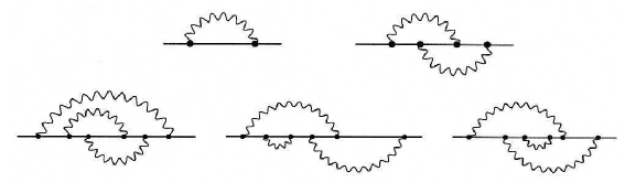
Figure 3: The diagrams, used for calculation of the function $G$

Thus, it order to find the function $G$ in the considered case it is necessary to calculate diagrams presented in Fig. 3. Then the function $G$ is obtained according to definition (104). One-, two- and three-loop parts of the function $G$, defined by diagrams in Fig. 3, will be denoted by $G_{1}$, $G_{2}$ and $G_{3}$ respectively. Expressions for them, obtained by calculating these diagrams, are

$$G_{1}=-2e^{2}\int\frac{d^{4}k}{(2\pi)^{4}}\,\Big{(}1+\frac{k^{2n}}{\Lambda^{2n}}\Big{)}^{-1}\,\frac{1}{k^{2}\,(q+k)^{2}};$$ (140)

$$G_{2}=-4e^{4}\int\frac{d^{4}k\,d^{4}l}{(2\pi)^{8}}\,\Big{(}1+\frac{k^{2n}}{\Lambda^{2n}}\Big{)}^{-1}\Big{(}1+\frac{l^{2n}}{\Lambda^{2n}}\Big{)}^{-1}\frac{(2q+k+l)^{2}}{k^{2}\,l^{2}(k+q)^{2}\,(q+l)^{2}\,(k+q+l)^{2}};$$

(141)

$$G_{3}=-4\,e^{6}\int\frac{d^{4}k\,d^{4}l\,d^{4}r}{(2\pi)^{12}}\,\Big{(}1+\frac{k^{2n}}{\Lambda^{2n}}\Big{)}^{-1}\Big{(}1+\frac{l^{2n}}{\Lambda^{2n}}\Big{)}^{-1}\Big{(}1+\frac{r^{2n}}{\Lambda^{2n}}\Big{)}^{-1}\times$$

$$\times\frac{1}{k^{2}l^{2}r^{2}(q+k)^{2}(q+l)^{2}(q+k+l)^{2}}\Bigg{(}\frac{(2q+2k+r+l)^{2}(q+l)^{2}}{(q+r+k)^{2}\,(q+r+k+l)^{2}}+$$

$$+\frac{(2q+k+l)^{2}}{(q+r+k+l)^{2}}+\frac{2(2q+k+l)^{2}}{(q+r+k)^{2}}\Bigg{)}.\qquad$$ (142)

The complete function $G$ (certainly without diagrams, which are not essential for this paper) in the considered approximation is given by

$$G(q^{2})=1+G_{1}+G_{2}+G_{3},$$ (143)

where the unity is a tree contribution.

The functions $F(q^{2})$ and $f(q^{2})$ are defined from three-point Green functions by Eq. (4.2). As in the case of the function $G$, in order to obtain a contribution, which corresponds to the considered class of the four-loop diagrams, it is sufficient to calculate only diagrams of a special form. They are obtained from diagrams, presented in Fig. 3, by all possible insertions of one external $V$-line. In all these diagrams one external straight line corresponds to the chiral field $\phi$ and the other corresponds to the non-chiral field $\phi^{*}_{0}$.

We will denote one-, two- and three-loop contributions to the function $f$ by $f_{1}$, $f_{2}$ and $f_{3}$ respectively. Similar notation we will use for the function $F$. Because in the tree approximation these functions are 0 and $f_{1}=0$, in the considered order we have

$$F=F_{1}+F_{2}+F_{3};\qquad f=f_{2}+f_{3}.$$ (144)

Expressions for $f_{1}$, $f_{2}$, $f_{3}$, $F_{1}$ and $F_{2}$, obtained by calculation of the above pointed diagrams have the following form:

$$f_{1}(q^{2})=0;\vphantom{\Big{(}}$$ (147)

$$f_{2}(q^{2})=\frac{1}{2}\,e^{4}\int\frac{d^{4}k\,d^{4}l}{(2\pi)^{8}}\,\Big{(}1+\frac{k^{2n}}{\Lambda^{2n}}\Big{)}^{-1}\Big{(}1+\frac{l^{2n}}{\Lambda^{2n}}\Big{)}^{-1}\,\times$$

$$\quad\quad\times\frac{1}{k^{2}\,l^{2}\,(k+q)^{2}\,(q+l)^{2}(k+q+l)^{2}}\times$$

$$\qquad\times\Bigg{(}-2+\frac{(2q+k+l)_{\mu}(k+q)^{\mu}}{(k+q)^{2}}+\frac{(2q+k+l)_{\mu}(l+q)^{\mu}}{(l+q)^{2}}\Bigg{)};$$

$$f_{3}(q^{2})=4\,e^{6}\int\frac{d^{4}k\,d^{4}l\,d^{4}r}{(2\pi)^{12}}\,\Big{(}1+\frac{k^{2n}}{\Lambda^{2n}}\Big{)}^{-1}\Big{(}1+\frac{l^{2n}}{\Lambda^{2n}}\Big{)}^{-1}\Big{(}1+\frac{r^{2n}}{\Lambda^{2n}}\Big{)}^{-1}\times$$

$$\times\frac{1}{k^{2}\,l^{2}\,r^{2}\,(k+q)^{2}\,(q+l)^{2}\,(q+k+l)^{2}}\,\Bigg{(}\frac{1}{(k+q+r)^{2}}+\frac{1}{2(k+l+q+r)^{2}}-$$

$$-\frac{(2q+k+l)^{\mu}(k+q)^{\mu}}{2(k+q)^{2}\,(k+q+r)^{2}}-\frac{(2q+k+l)^{\mu}(l+q)^{\mu}}{2(l+q)^{2}\,(k+q+r)^{2}}-\frac{(2q+k+l)^{\mu}(k+q)^{\mu}}{2(k+q)^{2}\,(k+l+q+r)^{2}}-\vphantom{\Bigg{(}}$$

$$-\frac{(2q+k+l)^{\mu}(k+q+r)^{\mu}}{2(k+q+r)^{4}}\Bigg{)}.$$

$$F_{1}(q^{2})=-\,\frac{e^{2}}{8}\int\frac{d^{4}k}{(2\pi)^{4}}\,\Big{(}1+\frac{k^{2n}}{\Lambda^{2n}}\Big{)}^{-1}\frac{1}{k^{2}\,(k+q)^{4}};$$ (148)

$$F_{2}(q^{2})=\frac{1}{4}\,e^{4}\int\frac{d^{4}k\,d^{4}l}{(2\pi)^{8}}\,\Big{(}1+\frac{k^{2n}}{\Lambda^{2n}}\Big{)}^{-1}\Big{(}1+\frac{l^{2n}}{\Lambda^{2n}}\Big{)}^{-1}\times$$

$$\times\frac{1}{k^{2}\,l^{2}\,(k+q)^{2}\,(q+l)^{2}(k+q+l)^{2}}\Bigg{(}4-2\,\frac{(q+l)^{2}}{(k+q)^{2}}-\,\frac{(2q+k+l)^{2}}{(q+k+l)^{2}}\Bigg{)}.$$ (149)

An expression for $F_{3}$ has been calculated, but it is not presented because it is very large. (It is not required for verification of identity (120).)

Using the obtained expressions it is possible to verify identity (120). With the considered accuracy we have

$$\frac{f}{q^{2}G}=\frac{1}{q^{2}}\Big{(}f_{3}-f_{2}\cdot G_{1}\Big{)}.$$ (150)

Substituting here expressions for the functions $G_{1}$, $f_{2}$ and $f_{3}$ from Eqs. (140), (147), (147) we obtain, that the integrand can be written as a total derivative with respect to the momentum $q$

$$\int\frac{d^{4}q}{(2\pi)^{4}}\,\frac{d}{d\ln\Lambda}\,\frac{f}{q^{2}G}=e^{6}\int\frac{d^{4}q\,d^{4}k\,d^{4}l\,d^{4}r}{(2\pi)^{16}}\,\frac{d}{d\ln\Lambda}\Bigg{[}\Big{(}1+\frac{k^{2n}}{\Lambda^{2n}}\Big{)}^{-1}\Big{(}1+\frac{l^{2n}}{\Lambda^{2n}}\Big{)}^{-1}\times\qquad$$

$$\times\Big{(}1+\frac{r^{2n}}{\Lambda^{2n}}\Big{)}^{-1}\Bigg{]}\frac{\partial}{\partial q^{\mu}}\left\{\frac{(2q+k+l)^{\mu}}{k^{2}l^{2}r^{2}q^{2}(k+q)^{2}(q+l)^{2}(q+r)^{2}(k+q+l)^{2}}\right\}.$$ (151)

This equality can be checked by calculating the derivative with respect to $q^{\mu}$ using the Leibnitz rule and comparing the result with Eq. (150), in which expressions for the functions $G_{1}$, $f_{2}$ and $f_{3}$ are obtained by explicit calculation of diagrams.

Because the integrand in Eq. (6.1) is a total derivative with respect to $q^{\mu}$ of the expression, which goes to 0 in the limit $q\to\infty$, expression (6.1) is 0. This means that identity (120) is correct in the considered approximation and for the considered class of diagrams.

Note that the equalities, present above, allow checking the method of summing Feynman diagrams by using the Schwinger-Dyson equations and Ward identities. For this purpose it is possible to calculate both effective diagrams in Eq. (102) in the four-loop approximation explicitly and compare the result with Eqs. (4.3) and (117). In considered approximation

$$\frac{1}{q^{2}}\,\frac{d}{dq^{2}}\ln(G^{2})=\frac{q^{\mu}}{q^{4}}\,\frac{\partial}{\partial q^{\mu}}\Big{(}G_{3}-G_{1}\cdot G_{2}\Big{)};$$ (152)

$$\frac{F}{q^{2}G}=\frac{1}{q^{2}}\Big{(}F_{3}-F_{2}\cdot G_{1}-F_{1}\cdot G_{2}\Big{)}.$$ (153)

Explicit calculations were made by the method, proposed in Ref. [46], which simplified finding a part of diagram, proportional to $V\partial^{2}\Pi_{1/2}V$. Nevertheless, it does not allow to obtain a part, proportional to $V^{2}$. That is why the verification of Eqs. (4.3) and (117) was made only for terms, proportional to $V\partial^{2}\Pi_{1/2}V$. In the both cases this verification completely confirms them.

As a small technical remark let us note, that making this verification it is necessary to take into account that a large number of ordinary Feynman diagrams contributes both to the first effective diagram in Eq. (102) and to the second one. For example, it is easy to see, that a contribution of a diagram, presented in Fig. 4

Figure 4: One of the diagrams, giving contribution to both effective diagrams

is divided into parts $3/4$ and $1/4$, which correspond to the first and to the second diagrams in Eq. (102).

6.2 Three-loop approximation in the non-Abelian case

The Feynman rules are different in a non-Abelian theory mostly due to vertexes with the selfaction of the gauge field. That is why it is desirable to check the new identity also in this case [47]. For diagrams that do not contain such vertexes the calculations are similar to the Abelian case. But for diagrams with the triple vertex of the gauge field an additional verification is very desirable. As we already mentioned, for this purpose it is not necessary to calculate all Feynman diagrams in a given order of the perturbation theory. It is sufficient to consider, for example, a typical three-loop diagram, presented in Fig. 5.

Figure 5: Diagram, generating considered contribution to the new identity

Figure 6: Way of cutting the diagram

From the topological point of view there is the only way to cut a loop of the matter superfield, presented in Fig. 6. Hence, it is necessary to calculate a set of diagrams, presented in Fig. 7. As earlier, in all these diagrams the chiral field $\phi$ is at the first external line and the non-chiral field $\phi^{*}_{0}$ is at the second line. Therefore, all presented diagrams are not topologically equivalent.

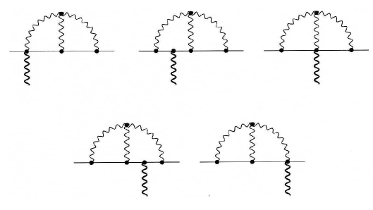
Figure 7: Diagrams, defining the function $f$, corresponding to the considered diagrams

Calculating these diagrams we can find the function $f$. The function $G$ in the lowest approximation should be set to 1. Really, in the tree approximation $G=1$. Hence, in the given order for the considered class of diagrams we have:

$$G(q^{2})=1+O(\alpha^{2});\qquad f(q^{2})=f_{2}(q^{2})+O(\alpha^{3}).$$ (154)

where $f_{2}$ is proportional to $\alpha^{2}$. Therefore,

$$\int d^{4}q\,\frac{d}{d\ln\Lambda}\frac{f(q^{2})}{q^{2}G(q^{2})}=\int d^{4}q\,\frac{d}{d\ln\Lambda}\frac{f_{2}(q)}{q^{2}}+O(\alpha^{3}).$$ (155)

So, we see that the considered contribution is actually determined by the two-loop value of the single function $f_{2}$.

In order to find the function $f_{2}$ in the two-loop approximation, it is necessary to make an explicit calculation of Feynman diagrams, presented in Fig. 7, using the standard supergraph technique. The result is (in the Euclidean space, after the Weak rotation)

$$f_{2}(q)=-2\pi^{2}\alpha^{2}C_{2}\Big{(}C_{2}(R)-\frac{1}{2}\,C_{2}\Big{)}\,\int\frac{d^{4}k\,d^{4}l}{(2\pi)^{8}}\Bigg{(}\frac{l^{\mu}}{(k+q+l)^{2}}+\frac{(k+q)^{\mu}}{(k+q)^{2}}\Bigg{)}\times$$ (156)

$$\times\frac{(k+q+l)_{\mu}}{(k+q)^{2}\,(k+q+l)^{2}k^{2}\Big{(}1+k^{2n}/\Lambda^{2n}\Big{)}\,l^{2}\Big{(}1+l^{2n}/\Lambda^{2n}\Big{)}\,(k+l)^{2}\Big{(}1+(k+l)^{2n}/\Lambda^{2n}\Big{)}},$$

where $C_{2}(R)$ and $C_{2}$ are defined by

$$T^{a}\,T^{a}=C_{2}(R),$$ (157)

$$f^{amn}\,f^{bmn}=C_{2}\,\delta^{ab}.$$ (158)

Substituting this expression into Eq. (155), we obtain that in the considered approximation for the considered diagrams

$$\int\frac{d^{4}q}{(2\pi)^{4}}\,\frac{d}{d\ln\Lambda}\frac{f(q^{2})}{q^{2}\,G(q^{2})}=$$

$$=\alpha^{2}\pi^{2}\,C_{2}\Big{(}C_{2}(R)-\frac{1}{2}\,C_{2}\Big{)}\,\int\frac{d^{4}q\,d^{4}k\,d^{4}l}{(2\pi)^{12}}\,\frac{\partial}{\partial q^{\mu}}\Bigg{\{}\Lambda\frac{d}{d\Lambda}\,\Bigg{[}\frac{(k+q+l)^{\mu}}{q^{2}\,(k+q)^{2}\,(k+q+l)^{2}}\times\qquad$$

$$\times\frac{1}{k^{2}\Big{(}1+k^{2n}/\Lambda^{2n}\Big{)}\,l^{2}\Big{(}1+l^{2n}/\Lambda^{2n}\Big{)}\,(k+l)^{2}\Big{(}1+(k+l)^{2n}/\Lambda^{2n}\Big{)}}\Bigg{]}\Bigg{\}}=0.$$ (159)

This means that the new identity for Green functions is also valid in the non-Abelian theory.

7 Conclusion

Our investigation of applying the higher derivative regularization to calculation of quantum corrections in supersymmetric theories allows revealing some interesting features, which were not noted earlier. We should first mention the completely unexpected result: all complicated integrals, defining the Gell-Mann–Low function, are integrals of total derivatives and can be easily calculated. It is important to note that with the higher derivative regularization the Gell-Mann–Low function is calculated in the simplest way. According to our calculations this is a function that coincides with the exact NSVZ $\beta$-function. So, it is not necessary to tune a renormalization scheme, as it was done earlier, calculating the $\beta$-function defined by divergence in the $\overline{MS}$-scheme with the dimensional reduction. Note that with the higher covariant derivative regularization there are divergences only in the one-loop approximation. In a certain degree this confirms speculations, presented in Ref. [37], in which the authors suggested that the Wilsonian action was exhausted at the one-loop. The calculations show that with the higher derivative regularization the renormalized action is exhausted at the one-loop.

The features, which appear calculating quantum corrections in supersymmetric theories, can be partially explained by substituting solutions of the Slavnov–Taylor identities into the Schwinger–Dyson equations. However, it is necessary to suppose existing a new identity for the Green functions, which does not follow from known symmetries of the theory. The exact $\beta$-function can be also considered as a similar identity. Quite possible that all such identities are consequences of some nontrivial symmetry. Existence of such symmetries was already proposed earlier [11] in $N=1$ finite supersymmetric theories. That is why the obtained results could be also useful for their investigation. In particular, it is possible that the anomalous dimension in $N=1$ finite theories is also an integral of a total derivative. Now this statement is being checked by the explicit calculation.

Finally, it is necessary to enumerate some interesting problems, which have not yet been solved. One of them is a proof of the new identity starting from some symmetry. May be, there is a relation between the considered problem and the AdS/CFT-correspondence. In favour of this we note that it is convenient to formulate the new identity in terms of vacuum expectation values of gauge invariant operators. Possibly it would be possible to derive the NSVZ $\beta$-function for the pure Yang–Mills theory exactly to all orders of the perturbation theory. In this case the Schwinger–Dyson equations are rather involved and their investigation is much more complicated.

To conclude, we can say that dynamics of supersymmetric theories is unexpectedly rich by the interesting features, which sometimes are hard to be explained. The higher covariant derivative regularization is an excellent tool for revealing these features.

Acknowledgments.

This paper was partially supported by the Russian Foundation for Basic Research (Grant No. 05-01-00541).

References

• [1] N.Seiberg, E.Witten, Nucl.Phys. B426, (1994), 19; erratum 430, (1994), 485.
• [2] M.Matone, Phys.Lett. B357, (1995), 342.
• [3] N.Dorey, V.Khoze, M.Mattis, Phys.Lett. B390, (1997), 205.
• [4] P.Howe, P.West, Nucl.Phys. B486, (1997), 425.
• [5] G.Bonelli, M.Matone, M.Tonin, Phys.Rev. D55, (1997), 6466.
• [6] J.Maldacena, Adv.Theor.Math.Phys. 2, (1998), 231.
• [7] V.Novikov, M.Shifman, A.Vainstein, V.Zakharov, Phys.Lett. 166B, (1985), 329.
• [8] L.V.Avdeev, O.V.Tarasov, Phys.Lett. 112 B, (1982), 356.
• [9] I.Jack, D.R.T.Jones, C.G.North, Nucl.Phys. B 473, (1996), 308.
• [10] I.Jack, D.R.T.Jones, C.G.North, Phys.Lett. 386 B, (1996), 138.
• [11] A.V.Ermushev, D.I.Kazakov, O.V.Tarasov, Nucl.Phys. B281, (1987), 72.
• [12] I.Jack, D.R.T.Jones, Regularization of supersymmetric theories, hep-ph/ 9707278.
• [13] G.t’Hooft, M.Veltman, Nucl.Phys. B44, (1972), 189.
• [14] W.Siegel, Phys.Lett. 84 B, (1979), 193.
• [15] W.Siegel, Phys.Lett. 94B, (1980), 37.
• [16] A.A.Slavnov, Theor.Math.Phys. 23, (1975), 3.
• [17] C.Martin, F.Ruiz Ruiz, Nucl.Phys. B 436, (1995), 645.
• [18] M.Asorey, F.Falceto, Phys.Rev D 54, (1996), 5290.
• [19] T.Bakeyev, A.Slavnov, Mod.Phys.Lett. A11, (1996), 1539.
• [20] P.Pronin, K.Stepanyantz, Phys.Lett. B414, (1997), 117.
• [21] A.Morozov, hep-th/0712.0946.
• [22] P.West, Introduction to supersymmetry and supergravity, World Scientific, 1986.
• [23] J.Gates, M.Grisaru, M.Rocek, W.Siegel, Front.Phys., 58, (1983), 1.
• [24] P.West, Nucl.Phys. B 268, (1986), 113.
• [25] A.A.Slavnov, Phys.Lett. B 518, (2001), 195.
• [26] A.A.Slavnov, Theor.Math.Phys. 130, (2002), 1.
• [27] A.A.Slavnov, K.V.Stepanyantz, Theor.Math.Phys., 135, (2003), 673.
• [28] A.A.Slavnov, K.V.Stepanyantz, Theor.Math.Phys., 139, (2004), 599.
• [29] H.Kluberg-Stern, J.B.Zuber, Phys.Rev. D12, (1975), 467.
• [30] H.Kluberg-Stern, J.B.Zuber, Phys.Rev. D12, (1975), 482.
• [31] L.D.Faddeev, A.A.Slavnov, Gauge fields, introduction to quantum theory, second edition, Benjamin, Reading, 1990.
• [32] A.Soloshenko, K.Stepanyantz, Theor.Math.Phys., 134, (2003), 377.
• [33] A.A.Soloshenko, K.V.Stepanyantz, hep-th/0304083. A brief version of this paper is A.Soloshenko, K.Stepanyantz, Theor.Math.Phys. 140, (2004), 1264.
• [34] A.Soloshenko, K.Stepanyantz, Two-loop renormalization of $N=1$ supersymmetric electrodynamics, regularized by higher derivatives, hep-th/0203118.
• [35] K.Stepanyantz, Theor.Math.Phys. 140, (2004), 939.
• [36] N.Arkani-Hamed, H.Murayama, JHEP 0006, (2000), 030.
• [37] M.Shifman, A.Vainstein, Nucl.Phys. B277, (1986), 456.
• [38] A.Pimenov, K.Stepanyantz, hep-th/0707.4006.
• [39] L.F.Abbott, M.T.Grisary, D.Zanon, Nucl.Phys. B244, (1984), 454.
• [40] J.Mas, M.Perez-Victoria, C.Seijas, JHEP, 0203, (2002), 049.
• [41] D.Z.Freedman, K.Johnson, J.I.Latorre, Nucl.Phys. B371, (1992), 353.
• [42] K.V.Stepanyantz, Theor.Math.Phys. 142, (2005), 29.
• [43] K.V.Stepanyantz, Theor.Math.Phys., 150, (2007), 377.
• [44] K.Stepanyantz, Theor.Math.Phys. 146, (2006), 321.
• [45] A.Pimenov, K.Stepanyantz, Theor.Math.Phys., 147, (2006), 687.
• [46] E.Andriyash, A.Pimenov, K.Stepanyantz Vestn.Mosk.Univ., Fiz.Astron., 4, (2005), 7.
• [47] A.Pimenov, K.Stepanyantz, hep-th/0710.5040.