Application of the Generalized Alignment Index (GALI) method to the dynamics of multi–dimensional symplectic maps

Abstract

We study the phase space dynamics of multi–dimensional symplectic maps, using the method of the Generalized Alignment Index (GALI). In particular, we investigate the behavior of the GALI for a system of $N=3$ coupled standard maps and show that it provides an efficient criterion for rapidly distinguishing between regular and chaotic motion.

1 Introduction

The distinction between regular and chaotic motion in conservative dynamical systems is fundamental in many areas of applied sciences. This distinction is particularly difficult in systems with many degrees of freedom, basically because it is not feasible to visualize their phase space. Thus, we need fast and accurate tools to obtain information about the chaotic vs. regular nature of the orbits of such systems and characterize efficiently large domains in their phase space as ordered, chaotic, or “sticky” (which lie between order and chaos).

In this paper we focus our attention on the method of the Generalized ALignment Index (GALI), which was recently introduced and applied successfully for the distinction between regular and chaotic motion in Hamiltonian systems [1]. The GALI method is a generalization of the Smaller Alignment Index (SALI) technique of chaos detection [2, 3, 4]. We present some preliminary results of the application of GALIs on the dynamical study of symplectic maps, considering in particular the case of a 6–dimensional (6D) system of three coupled standard maps [5]. It is important to note that maps of this type have been extensively studied in connection with the problem of the stability of hadron beams in high energy accelerators, see [6] and references therein.

Our numerical results reported here verify the theoretically predicted behavior of GALIs obtained in [1] for Hamiltonian systems. In addition we study in more detail the behavior of chaotic orbits which visit different regions of chaoticity in the phase space of our system.

2 Definition and behavior of GALI

Let us first briefly recall the definition of GALI and its behavior for regular and chaotic motion, adjusting the results obtained in [1] to symplectic maps. Considering a 2$N$–dimensional map, we follow the evolution of an orbit (using the equations of the map) together with $k$ initially linearly independent deviation vectors of this orbit $\overrightarrow{\nu}_{1},\overrightarrow{\nu}_{2},...,\overrightarrow{\nu}_{k}$ with $2\leq k\leq 2N$ (using the equations of the tangent map). The Generalized ALignment Index of order $k$ is defined as the norm of the wedge or exterior product of the $k$ unit deviation vectors:

$$GALI_{k}(n)=\parallel\hat{\nu}_{1}(n)\wedge\hat{\nu}_{2}(n)\wedge...\wedge\hat{\nu}_{k}(n)\parallel$$ (1)

and corresponds to the volume of the generalized parallelepiped, whose edges are these $k$ vectors. We note that the hat ($\,\hat{}\,$) over a vector denotes that it is of unit magnitude and that $n$ is the discrete time.

In the case of a chaotic orbit all deviation vectors tend to become linearly dependent, aligning in the direction of the eigenvector which corresponds to the maximal Lyapunov exponent and GALI_k tends to zero exponentially following the law [1]:

$$GALI_{k}(n)\propto e^{-[(\sigma_{1}-\sigma_{2})+(\sigma_{1}-\sigma_{3})+...+(\sigma_{1}-\sigma_{k})]n},$$ (2)

where $\sigma_{1},\ldots,\sigma_{k}$ are approximations of the first $k$ largest Lyapunov exponents. In the case of regular motion on the other hand, all deviation vectors tend to fall on the $N$–dimensional tangent space of the torus on which the motion lies. Thus, if we start with $k\leq N$ general deviation vectors they will remain linearly independent on the $N$–dimensional tangent space of the torus, since there is no particular reason for them to become aligned. As a consequence GALI_k remains practically constant for $k\leq N$. On the other hand, GALI_k tends to zero for $k>N$, since some deviation vectors will eventually become linearly dependent, following a power law which depends on the dimensionality of the torus on which the motion lies and on the number $m$ ($m\leq N$ and $m\leq k$) of deviation vectors initially tangent to this torus. So, the behavior of GALI_k for regular orbits is given by [1, 7]

$$GALI_{k}(n)\propto\left\{\begin{array}[]{ll}constant&\hbox{if $2\leq k\leq N$}\\ \frac{1}{n^{2(k-N)-m}}&\hbox{if $N<k\leq 2N$ and $0\leq m<k-N$}\\ \frac{1}{n^{k-N}}&\hbox{if $N<k\leq 2N$ and $m\geq k-N$}\end{array}.\right.$$ (3)

3 Dynamical study of a 6D standard map

As a model for our study we consider the 6D map:

$$\begin{array}[]{lll}x_{1}^{\prime}&=&x_{1}+x_{2}^{\prime}\\ x_{2}^{\prime}&=&x_{2}+\frac{K}{2\pi}\sin(2\pi x_{1})-\frac{\beta}{2\pi}\{\sin[2\pi(x_{5}-x_{1})]+\sin[2\pi(x_{3}-x_{1})]\}\\ x_{3}^{\prime}&=&x_{3}+x_{4}^{\prime}\\ x_{4}^{\prime}&=&x_{4}+\frac{K}{2\pi}\sin(2\pi x_{3})-\frac{\beta}{2\pi}\{\sin[2\pi(x_{1}-x_{3})]+\sin[2\pi(x_{5}-x_{3})]\}\\ x_{5}^{\prime}&=&x_{5}+x_{6}^{\prime}\\ x_{6}^{\prime}&=&x_{6}+\frac{K}{2\pi}\sin(2\pi x_{5})-\frac{\beta}{2\pi}\{\sin[2\pi(x_{1}-x_{5})]+\sin[2\pi(x_{3}-x_{5})]\}\end{array}$$ (4)

which consists of three coupled standard maps [5] and is a typical nonlinear system, in which regions of chaotic and quasi–periodic dynamics are found to coexist. Note that each coordinate is given modulo 1 and that in our study we fix the parameters of the map (4) to $K=3$ and $\beta=0.1$.

In order to verify numerically the validity of equations (2) and (3), we shall consider two typical orbits of map (4), a chaotic one with initial condition $x_{1}=x_{3}=x_{5}=0.8$, $x_{2}=0.05$, $x_{4}=0.21$, $x_{6}=0.01$ (orbit C1) and a regular one with initial condition $x_{1}=x_{3}=x_{5}=0.55$, $x_{2}=0.05$, $x_{4}=0.01$, $x_{6}=0$ (orbit R1). In figure 1 we see the evolution of GALI_k, $k=2,\ldots,6$, for these two orbits.

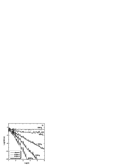
Figure 1: The evolution of GALI_k, $k=2,\ldots,6$, with respect to the number of iteration $n$ for a) the chaotic orbit C1 and b) the regular orbit R1. The plotted lines correspond to functions proportional to $e^{-(\sigma_{1}-\sigma_{2})n}$, $e^{-(2\sigma_{1}-\sigma_{2}-\sigma_{3})n}$, $e^{-(3\sigma_{1}-\sigma_{2})n}$, $e^{-4\sigma_{1}n}$, $e^{-6\sigma_{1}n}$ for $\sigma_{1}=0.70$, $\sigma_{2}=0.57$, $\sigma_{3}=0.32$ in a) and proportional to $n^{-2}$, $n^{-4}$, $n^{-6}$ in b).

It is well–known that in the case of symplectic maps the Lyapunov exponents are ordered in pairs of opposite signs [8]. Thus, for a chaotic orbit of the 6D map (4) we have $\sigma_{1}=-\sigma_{6}$, $\sigma_{2}=-\sigma_{5}$, $\sigma_{3}=-\sigma_{4}$ with $\sigma_{1}\geq\sigma_{2}\geq\sigma_{3}\geq 0$. So for the evolution of GALI_k, equation (2) gives

$$\begin{array}[]{c}\mbox{GALI}_{2}(n)\propto e^{-(\sigma_{1}-\sigma_{2})n},\,\,\,\mbox{GALI}_{3}(n)\propto e^{-(2\sigma_{1}-\sigma_{2}-\sigma_{3})n},\\ \mbox{GALI}_{4}(n)\propto e^{-(3\sigma_{1}-\sigma_{2})n},\,\,\,\mbox{GALI}_{5}(n)\propto e^{-4\sigma_{1}n},\,\,\,\mbox{GALI}_{6}(n)\propto e^{-6\sigma_{1}n}.\end{array}$$ (5)

The positive Lyapunov exponents of the chaotic orbit C1 were found to be $\sigma_{1}\approx 0.70$, $\sigma_{2}\approx 0.57$, $\sigma_{3}\approx 0.32$. From the results of figure 1a) we see that the functions of equation (5) for $\sigma_{1}=0.70$, $\sigma_{2}=0.57$, $\sigma_{3}=0.32$ approximate quite accurately the computed values of GALIs.

For the regular orbit R1 we first considered the general case where no initial deviation vector is tangent to the torus where the orbit lies. Thus, for the behavior of GALI_k, $k=2,\ldots,6$, equation (3) yields for $m=0$

$$\begin{array}[]{c}\mbox{GALI}_{2}(n)\propto\mbox{constant},\,\,\,\mbox{GALI}_{3}(n)\propto\mbox{constant},\,\,\,\mbox{GALI}_{4}(n)\propto\frac{1}{n^{2}},\\ \mbox{GALI}_{5}(n)\propto\frac{1}{n^{4}},\,\,\,\mbox{GALI}_{6}(n)\propto\frac{1}{n^{6}}.\end{array}$$ (6)

From the results of figure 1b) we see that the approximations appearing in (6) describe very well the evolution of GALIs.

In order to verify the validity of equation (3) for $1\leq m\leq 3$, in the case of regular motion, we evolve orbit R1 and three random initial deviation vectors for a large number of iterations (in our case for $5\times 10^{7}$ iterations), in order for the three deviation vectors to fall on the tangent space of the torus. Considering the current coordinates of the orbit as initial conditions and using $m=1$ or $m=2$ or $m=3$ of these vectors (that lie on the tangent space of the torus) as initial deviation vectors we start the computation of GALIs’ evolution. We note that the rest $6-m$ initial deviation vectors needed for our computation are randomly generated so that they do not lie on the tangent space of the torus. The results of these calculations are presented in figure 2, where the evolution of GALI_k, $k=2,\ldots,6$, for different values of $m$ is plotted. Figure 2 clearly illustrates that equation (3) describes accurately the behavior of GALIs for regular motion also in the case where some of the initial deviation vectors are chosen in the tangent space of the torus.

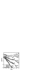
Figure 2: Evolution of GALI_k, $k=2,\ldots,6$, for the regular orbit R1 on a log–log scale, for different values of the number $m$ of deviation vectors initially tangent on the torus on which the motion occurs: a) $m=1$, b) $m=2$, c) $m=3$. In every panel lines corresponding to particular power laws are also plotted.

Let us now consider the case of a chaotic orbit which visits different regions of chaoticity in the phase space of the map. The orbit with initial conditions $x_{1}=x_{3}=x_{5}=0.55$, $x_{2}=0.05$, $x_{4}=0.21$, $x_{6}=0.0$ (orbit C2) exhibits this behavior as can be seen from the projections of its first $1000$ successive consequents on different 2–dimensional planes plotted in figure 3.

Figure 3: Projections on the planes a) $(x_{1},x_{2})$, b) $(x_{3},x_{4})$ and c) $(x_{5},x_{6})$ of the first $1000$ successive points of the chaotic orbit C2.

The projections look erratic, indicating that the orbit is chaotic. However, we also observe in all three projections that the C2 stays ‘trapped’ for many iterations in two oval–shaped regions and eventually escapes entering the big chaotic sea around these regions. This behavior is also depicted in the evolution of the Lyapunov exponents of the orbit (see figure 4a). The three positive Lyapunov exponents are seen to fluctuate around $\sigma_{1}\approx 0.033$, $\sigma_{2}\approx 0.02$, $\sigma_{3}\approx 0.005$ for about $1000$ iterations exhibiting ‘jumps’ to higher values when the orbit enters the big chaotic sea, stabilizing around $\sigma_{1}\approx 0.793$, $\sigma_{2}\approx 0.624$, $\sigma_{3}\approx 0.365$.

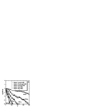
Figure 4: a) The evolution of the three positive Lyapunov exponents of the chaotic orbit C2. The evolution of GALI_k, $k=2,\ldots,6$, with respect to the number of iteration $n$ for the same orbit when we use as initial condition of the orbit its coordinates at b) $n=0$ and at c) $n=10^{6}$ iterations. The plotted lines in b) and c) correspond to functions proportional to $e^{-(\sigma_{1}-\sigma_{2})n}$, $e^{-(2\sigma_{1}-\sigma_{2}-\sigma_{3})n}$, $e^{-(3\sigma_{1}-\sigma_{2})n}$, $e^{-4\sigma_{1}n}$, $e^{-6\sigma_{1}n}$ for $\sigma_{1}=0.033$, $\sigma_{2}=0.02$, $\sigma_{3}=0.005$ in b) and $\sigma_{1}=0.793$, $\sigma_{2}=0.624$, $\sigma_{3}=0.365$ in c).

Let us now study how the GALIs are influenced by the fact that orbit C2 visits two different regions of chaoticity characterized by different values of Lyapunov exponents. Since C2 is a chaotic orbit, its GALIs should tend exponentially to zero following the laws of equation (5). Thus, starting the computation of the GALI_k, $k=2,\ldots,6$, from an initial point of C2 located in the first chaotic sea, we see that the slopes of the exponential decay of GALIs are well described by equation (5) using for $\sigma_{1}$, $\sigma_{2}$, $\sigma_{3}$ the approximate values of the Lyapunov exponents of the small chaotic region (figure 4b). On the other hand, using as initial condition for this chaotic orbit its coordinates after $10^{6}$ iterations, when the orbit has escaped in the second chaotic region, the evolution of GALIs is again well approximated by equation (5) but this time for $\sigma_{1}=0.793$, $\sigma_{2}=0.624$, $\sigma_{3}=0.365$, which are the approximations of the Lyapunov exponents of the big chaotic sea (figure 4c). Thus, we see that in this case also the $\sigma_{i}$, $i=1,\ldots,k$ which appear in equation (5) are good approximations of the first $k$ Lyapunov exponents of the large chaotic region in which the orbit eventually wanders after about $10^{3}$ iterations.

4 Conclusions

In this paper we verified the theoretically predicted behavior of the Generalized Alignment Index (GALI) by considering some particular regular and chaotic orbits of a $2N$–dimensional symplectic map with $N=3$. In particular, we showed numerically that all GALI_k, $2\leq k\leq 2N$, tend to zero exponentially for chaotic orbits, while for regular orbits they remain different from zero for $2\leq k\leq N$ and tend to zero, following particular power laws, for $N<k\leq 2N$. Thus, by using GALI_k with sufficiently large $k$, one can infer quickly the nature of the dynamics much faster than it is possible by using other methods.

Also, the study of chaotic orbits which visit different regions of chaoticity in the phase space of the system, provides further evidence that the exponents of the exponential decay of GALIs are related to the local values of Lyapunov exponents. Thus, we have shown that the different behaviors of the GALIs for regular and chaotic orbits can be used for the fast and accurate identification of regions of chaoticity and regularity in the phase space of symplectic maps. We plan to investigate this further in a future publication concerning maps with $N>>3$, which describe arrays of conservative nonlinear oscillators.

5 Acknowledgments

T. Manos was partially supported by the “Karatheodory” graduate student fellowship No B395 of the University of Patras, the program “Pythagoras II” and the Marie Curie fellowship No HPMT-CT-2001-00338. Ch. Skokos was supported by the Marie Curie Intra–European Fellowship No MEIF–CT–2006–025678. The first author (T. M.) would also like to express his gratitude to the Institut de Mécanique Céleste et de Calcul des Ephémérides (IMCCE) of the Observatoire de Paris for its excellent hospitality during his visit in June 2006, when part of this work was completed.

References

- [1] Ch. Skokos, T. Bountis and Ch. Antonopoulos, Physica D, 231, 30, (2007).
- [2] Ch. Skokos, J. Phys. A: Math. Gen., 34, 10029, (2001).
- [3] Ch. Skokos, Ch. Antonopoulos, T. Bountis and M. Vrahatis, Prog. Theor. Phys. Suppl., 150, 439, (2003).
- [4] Ch. Skokos, Ch. Antonopoulos, T. Bountis and M. Vrahatis, J. Phys. A, 37, 6269, (2004).
- [5] H. Kantz and P. Grassberger, J. Phys. A: Math. Gen, 21 L127, (1988).
- [6] T. Bountis and Ch. Skokos, Nucl. Instr. Meth. Phys. Res. A, 561, 173, (2006).
- [7] H. Christodoulidi and T. Bountis, ROMAI Journal, 2, 2, (2007).
- [8] M. A. Lieberman and A. J. Lictenberg, Regular and Chaotic Dynamics, Springer–Verlag, (1992).