Link Scheduling in STDMA Wireless Networks: A Line Graph Approach

Abstract

We consider point to point link scheduling in Spatial Time Division Multiple Access (STDMA) wireless networks under the physical interference model. We propose a novel link scheduling algorithm based on a line graph representation of the network, by embedding the interferences between pairs of nodes into the edge weights of the line graph. Our algorithm achieves lower schedule length and lower run time complexity than existing algorithms.

I Introduction

A prevalent scheme for spatial reuse in wireless networks is Spatial Time Division Multiple Access (STDMA) [1], in which time is divided into fixed-length slots that are organized cyclically. An STDMA link schedule defines the transmission rights for each time slot in such a way that communicating pairs of nodes, i.e., links, assigned to the same time slot do not collide. The interference between the links can be modeled by assuming that transmission on a link is successful if the distance between the nodes is less than some communication range and no other node is transmitting within an interference range from the receiver of the link. This is called protocol interference model [2]. Under these assumptions, the network can be modeled by a communication graph and scheduling algorithms employ edge coloring techniques to minimize the schedule length. Though determining an optimal schedule is known to be NP-complete [3], heuristics have been proposed in [3], [4], [5].

A more realistic model would be to consider a transmission on a link to be successful if the Signal to Interference and Noise Ratio (SINR) at the receiver is greater than some threshold, say $\gamma_{c}$. This model is called physical interference model [2]. Recently, few authors [6], [7], [8], [9] have proposed scheduling algorithms based on this physical interference model, which result in improved network throughput. In [6], the authors propose a polynomial time algorithm which gives a provable performance guarantee within a constant factor compared to the optimal. This algorithm is a greedy heuristic that determines a schedule based on the feasibility of satisfying SINR conditions using a communication graph based representation of the network.

In this paper, we propose a novel scheduling algorithm for STDMA wireless networks under physical interference model. Our approach is based on a line graph [10] representation of the network where the weights of the edges correspond to interferences between pairs of nodes. Analogous to a line graph, a conflict graph model under physical interference assumptions has been suggested in [11]. However, the authors of [11] do not propose any specific scheduling algorithm and use the weighted conflict graph only to compute bounds on the network throughput. On the other hand, we use a line graph representation of the network under the physical interference model and develop a novel scheduling algorithm with lower time complexity and substantially improved performance in terms of schedule length.

The rest of the paper is organized as follows. In Section II, we explain our system model, formulate the problem and describe the proposed algorithm. In Section III, we prove the correctness of our algorithm and derive its computational complexity. The performance of our algorithm is evaluated in Section IV. We conclude in Section V.

II Line graph based link scheduling algorithm

Consider an STDMA wireless network $\Upsilon(\cdot)$ with $N$ static nodes (wireless routers) in a two-dimensional plane. During a time slot, a node can transmit to exactly one node, receive from exactly one node or remain idle. We assume homogeneous and backlogged nodes. Let:

$$P =$$ transmission power of every node

$$N_{0} =$$ thermal noise power spectral density

$$\alpha =$$ path loss factor

The received signal power at a distance $d$ from a transmitter is given by $\frac{P}{d^{\alpha}}$. The STDMA wireless network $\Upsilon(\cdot)$ is modeled by its communication graph $\mathcal{G}(\mathcal{V},\mathcal{E})$, where $\mathcal{V}$ and $\mathcal{E}$ denote the sets of vertices and edges respectively, as follows:

1. Every node $i$ in $\Upsilon(\cdot)$ is represented by a vertex $v_{i}\in\mathcal{V}$ in $\mathcal{G}(\cdot)$.

2. If the Euclidean distance between two distinct nodes $a$ and $b$ is no greater than the communication range $R_{c}:=(\frac{P}{N_{0}\gamma_{c}})^{\frac{1}{\alpha}}$, then there is a directed edge from $v_{a}$ to $v_{b}$ in $\mathcal{G}(\cdot)$, i.e., $(v_{a},v_{b})\in\mathcal{E}$.

The set of edges in $\mathcal{G}(\cdot)$ to be scheduled is determined by a routing algorithm. For simplicity, we only consider exhaustive schedules, i.e., schedules which assign exactly one time slot to every directed edge in $\mathcal{G}(\cdot)$.

Algorithm 1 LineGraphLinkSchedule (LGLS)

1:  Input: Communication graph ${\mathcal{G}}$(${\mathcal{V}}$,${\mathcal{E}}$), $\gamma_{c}$, $N_{0}$, $P$

2:  Output: A coloring ${\mathcal{C}}$: ${\mathcal{E}}\rightarrow\{1,2,\ldots\}$

3:  ${\mathcal{V}^{\prime}}\leftarrow{\mathcal{E}}$ {Phase 1 begins}

4:  $\mbox{Construct the directed complete graph }{\mathcal{G}^{\prime}}({\mathcal{V}^{\prime}},{\mathcal{E}^{\prime}})$

5:  for all $e^{\prime}_{ij}\in{\mathcal{E}^{\prime}}$ do

6:     if $\mbox{edges }i\mbox{ and }j\mbox{ have a common vertex in }{\mathcal{G}(\cdot)}$ then

7:        $w_{ij}\leftarrow 1$

8:     else

9:        $w_{ij}\leftarrow\gamma_{c}\frac{{d(t_{j},r_{j})}^{\alpha}}{{d(t_{i},r_{j})}^{\alpha}}$

10:     end if

11:  end for{Phase 1 ends}

12:  for all $e^{\prime}_{ij}\in{\mathcal{E}^{\prime}}$ do {Phase 2 begins}

13:     $w^{\prime}(e^{\prime}_{ij})\leftarrow\max\{0,1-w_{ij}\}$

14:  end for{Phase 2 ends}

15:  for all $v_{j}^{\prime}\in{\mathcal{V}^{\prime}}$ do {Phase 3 begins}

16:     ${\mathcal{N}}(v_{j}^{\prime})\leftarrow\frac{N_{0}\gamma_{c}}{P}{{d(t_{j},r_{j})}^{\alpha}}$

17:  end for{Phase 3 ends}

18:  ${\mathcal{V}_{uc}^{\prime}}\leftarrow{\mathcal{V}^{\prime}}$ {Phase 4 begins}

19:  $p\leftarrow 0$

20:  while ${\mathcal{V}_{uc}^{\prime}}\neq\phi$ do

21:     $p\leftarrow p+1$

22:     $\mbox{choose }v^{\prime}\in{\mathcal{V}_{uc}^{\prime}}$ randomly

23:     ${\mathcal{C}}(v^{\prime})\leftarrow p$

24:     ${\mathcal{V}_{uc}^{\prime}}\leftarrow{\mathcal{V}_{uc}^{\prime}}\setminus\{v^{\prime}\}$

25:     ${\mathcal{V}_{p}^{\prime}}\leftarrow\{v^{\prime}\}$

26:     $\psi\leftarrow\mbox{1}$

27:     while $\psi=1\mbox{ and }{\mathcal{V}_{uc}^{\prime}}\neq\phi$ do

28:        $u^{\prime}\leftarrow\arg\max_{y^{\prime}\in{\mathcal{V}}_{uc}^{\prime}}\sum_{x^{\prime}\in{\mathcal{V}}_{p}^{\prime}}w^{\prime}(e^{\prime}_{x^{\prime}y^{\prime}})+w^{\prime}(e^{\prime}_{y^{\prime}x^{\prime}})$

29:        for all $v_{c}^{\prime}\in{\mathcal{V}_{p}^{\prime}}$ do

30:           if $\sum_{v_{1}^{\prime}\in{\mathcal{V}_{p}^{\prime}}\setminus\{v_{c}^{\prime}\}\cup\{u^{\prime}\}}w^{\prime}(e^{\prime}_{{v_{1}^{\prime}}{v_{c}^{\prime}}})\leqslant|{\mathcal{V}_{p}^{\prime}}|+{\mathcal{N}}(v_{c}^{\prime})-1$ then

31:              $\psi\leftarrow 0$

32:           end if

33:        end for

34:        if $\psi=1\mbox{ and }\sum_{v_{1}^{\prime}\in{\mathcal{V}_{p}^{\prime}}}w^{\prime}(e^{\prime}_{{v_{1}^{\prime}}u^{\prime}})>|{\mathcal{V}_{p}^{\prime}}|+{\mathcal{N}}(u^{\prime})-1$ then

35:           ${\mathcal{C}}(u^{\prime})\leftarrow p$

36:           ${\mathcal{V}_{p}^{\prime}}\leftarrow{\mathcal{V}_{p}^{\prime}}\cup\{u^{\prime}\}$

37:           ${\mathcal{V}_{uc}^{\prime}}\leftarrow{\mathcal{V}_{uc}^{\prime}}\setminus\{u^{\prime}\}$

38:        else

39:           $\psi\leftarrow 0$

40:        end if

41:     end while

42:  end while{Phase 4 ends}

We now motivate our Line Graph based Link Scheduling (LGLS) algorithm, and provide the pseudocode in Algorithm 1. In Phase 1, we first construct a directed complete line graph [10] ${\mathcal{G}^{\prime}}({\mathcal{V}^{\prime}},{\mathcal{E}^{\prime}})$ which has the edges of ${\mathcal{G}}(\cdot)$ as its vertices, i.e., ${\mathcal{V}^{\prime}}={\mathcal{E}}$. Let the edges of ${\mathcal{G}}(\cdot)$ and the corresponding vertices of ${\mathcal{G}^{\prime}}(\cdot)$ be labeled $1,2,\ldots,e$. Let $t_{i}$ and $r_{i}$ denote the transmitter and receiver respectively of edge $i$ in ${\mathcal{G}}(\cdot)$. Let $d(t_{i},r_{j})$ denote the Euclidean distance between $t_{i}$ and $r_{j}$.

For any two edges $i$ and $j$ in graph ${\mathcal{G}}(\cdot)$, the weight function $w_{ij}$ is defined as:

$$\begin{split}w_{ij}&=\begin{cases}1&\text{if }i\text{ and }j\text{ have a common vertex},\\ \gamma_{c}\frac{{d(t_{j},r_{j})}^{\alpha}}{{d(t_{i},r_{j})}^{\alpha}}&\text{otherwise.}\end{cases}\end{split}$$

This weight function $w_{ij}$ indicates the interference energy at $r_{j}$ due to transmission from $t_{i}$ to $r_{i}$ scaled with respect to the signal energy of $t_{j}$ at $r_{j}$.

In Phase 2, we compute the co-schedulability weight function $w^{\prime}(\cdot)$. For any two edges $i$ and $j$ in $\mathcal{G}(\cdot)$, the weight of the edge $e^{\prime}_{ij}$ in ${\mathcal{G}^{\prime}}(\cdot)$ is given by $w^{\prime}(e^{\prime}_{ij})=\max\{0,1-w_{ij}\}$. Since $w_{ij}$ and $w_{ji}$ represent the interference between links $i$ and $j$ in $\Upsilon(\cdot)$, $w^{\prime}(e^{\prime}_{ij})$ and $w^{\prime}(e^{\prime}_{ji})$ intuitively represent the co-schedulability of vertices $i$ and $j$ in $\mathcal{G}^{\prime}(\cdot)$. For example, if $w_{ij}$ is greater than or equal to $1$, it means that the interference between links $i$ and $j$ in $\Upsilon(\cdot)$ is very high and these links cannot be scheduled simultaneously. This will result in $w^{\prime}(e^{\prime}_{ij})$ being equal to $0$ indicating that the vertices $i$ and $j$ in $\mathcal{G}^{\prime}(\cdot)$ are not co-schedulable. On the other hand, if $w_{ij}$ is almost $0$, $w^{\prime}(e^{\prime}_{ij})$ will be almost $1$ indicating that the vertices $i$ and $j$ in $\mathcal{G}^{\prime}(\cdot)$ are co-schedulable. In Phase 3, we determine the normalized noise power at the receiver of each vertex of ${\mathcal{G}^{\prime}}(\cdot)$.

Our objective is to color the vertices of ${\mathcal{G}^{\prime}}(\cdot)$ (equivalently, edges of $\mathcal{G}(\cdot)$) using minimum number of colors under the physical interference model, i.e., subject to the condition that the SINR at every receiver of each link in $\Upsilon(\cdot)$ is greater than the communication threshold $\gamma_{c}$. Equivalently, for any ${\mathcal{V}_{cc}^{\prime}}\subseteq{\mathcal{V}^{\prime}}$, the coloring of all nodes $v_{i}^{\prime}\in{\mathcal{V}_{cc}^{\prime}}$ with the same color is defined to be feasible if

$$\frac{\frac{P}{{d(t_{v_{i}^{\prime}},r_{v_{i}^{\prime}})}^{\alpha}}}{N_{0}+\sum_{v_{j}^{\prime}\in{\mathcal{V}_{cc}^{\prime}}\setminus\{v_{i}^{\prime}\}}\frac{P}{{d(t_{v_{j}^{\prime}},r_{v_{i}^{\prime}})}^{\alpha}}}\geqslant\gamma_{c}\;\forall\;v_{i}^{\prime}\in{\mathcal{V}_{cc}^{\prime}}$$ (1)

In $\mathcal{G}^{\prime}(\cdot)$, this condition translates to the sum of weights of edges incoming to a vertex from all the co-colored vertices being greater than the sum of the number of remaining co-colored vertices and the normalized noise power minus a constant factor (unity).

The actual coloring of vertices of $\mathcal{G}^{\prime}(\cdot)$, i.e., edges of $\mathcal{G}(\cdot)$, occurs in Phase 4. Let ${\mathcal{V}_{uc}^{\prime}}$ at any time denote the set of uncolored vertices of $\mathcal{G}^{\prime}(\cdot)$ till that time. Initially, $\mathcal{V}_{uc}^{\prime}$ includes all the vertices of $\mathcal{G}^{\prime}(\cdot)$. First we choose a vertex randomly from ${\mathcal{V}_{uc}^{\prime}}$. This is assigned a new color, let it be $p$. Then we choose that vertex from ${\mathcal{V}_{uc}^{\prime}}$ which maximizes the sum of weights of all the edges between that vertex and the vertices colored by $p$. Now for each vertex colored with $p$, we check if the sum of weights of all the incoming edges is greater than the sum of the number of vertices colored with $p$ and the normalized noise power minus a constant factor (unity). If it is satisfied, the vertex is colored with $p$. If not, it is colored with a new color. The algorithm exits when all the vertices are colored.

III Analysis of LGLS Algorithm

In this section, we prove the correctness of the LGLS algorithm and derive its run time (computational) complexity. We follow the notation of Algorithm 1.

Theorem 1

For any ${\mathcal{V}_{cc}^{\prime}}\subseteq{\mathcal{V}^{\prime}}$, if $\sum_{v_{2}^{\prime}\in{\mathcal{V}_{cc}^{\prime}}\setminus\{v_{1}^{\prime}\}}w^{\prime}(e^{\prime}_{v_{2}^{\prime}v_{1}^{\prime}})$ $>|{\mathcal{V}_{cc}^{\prime}}|+{\mathcal{N}}(v_{1}^{\prime})-2$ $\;\forall\;v_{1}^{\prime}\in{\mathcal{V}_{cc}^{\prime}}$, then the coloring of all the vertices of ${\mathcal{V}_{cc}^{\prime}}$ with the same color is feasible.

Proof:

$w^{\prime}(e^{\prime}_{v_{2}^{\prime}v_{1}^{\prime}})\in[0,1]$. Suppose $w^{\prime}(e^{\prime}_{v_{3}^{\prime}v_{1}^{\prime}})=0$ for some $v_{1}^{\prime},v_{3}^{\prime}\in{\mathcal{V}_{cc}^{\prime}}$, $v_{1}^{\prime}\neq v_{3}^{\prime}$, then $\sum_{v_{2}^{\prime}\in{\mathcal{V}_{cc}^{\prime}}\setminus\{v_{1}^{\prime}\}}w^{\prime}(e^{\prime}_{v_{2}^{\prime}v_{1}^{\prime}})=$ $\sum_{v_{2}^{\prime}\in{\mathcal{V}_{cc}^{\prime}}\setminus\{v_{1}^{\prime},v_{3}^{\prime}\}}w^{\prime}(e^{\prime}_{v_{2}^{\prime}v_{1}^{\prime}})\leqslant$ $\sum_{v_{2}^{\prime}\in{\mathcal{V}_{cc}^{\prime}}\setminus\{v_{1}^{\prime},v_{3}^{\prime}\}}1=$ $|{\mathcal{V}_{cc}^{\prime}}\setminus\{v_{1}^{\prime},v_{3}^{\prime}\}|=|{\mathcal{V}_{cc}^{\prime}}|-2$, which contradicts the hypothesis. So, an edge connecting any two vertices in ${\mathcal{V}_{cc}^{\prime}}$ has positive weight. But, $w^{\prime}(e^{\prime}_{v_{2}^{\prime}v_{1}^{\prime}})=0$ or $1-w_{v_{2}^{\prime}v_{1}^{\prime}}$. So, $w^{\prime}(e^{\prime}_{v_{2}^{\prime}v_{1}^{\prime}})=1-w_{v_{2}^{\prime}v_{1}^{\prime}}\;\forall\;v_{1}^{\prime},v_{2}^{\prime}\in{\mathcal{V}_{cc}^{\prime}}$, $v_{1}^{\prime}\neq v_{2}^{\prime}$ and $w_{v_{2}^{\prime}v_{1}^{\prime}}<1\;\forall\;v_{1}^{\prime},v_{2}^{\prime}\in{\mathcal{V}_{cc}^{\prime}}$, $v_{1}^{\prime}\neq v_{2}^{\prime}$. If two vertices $v_{1}^{\prime},v_{2}^{\prime}\in{\mathcal{V}_{cc}^{\prime}}$ have a common vertex in $\mathcal{G}(\cdot)$, then $w_{v_{2}^{\prime}v_{1}^{\prime}}=1$, which is a contradiction. So no two vertices in ${\mathcal{V}_{cc}^{\prime}}$ have a common vertex in $\mathcal{G}(\cdot)$. From the hypothesis,
$\sum_{v_{2}^{\prime}\in{\mathcal{V}_{cc}^{\prime}}\setminus\{v_{1}^{\prime}\}}w^{\prime}(e^{\prime}_{v_{2}^{\prime}v_{1}^{\prime}})>|{\mathcal{V}_{cc}^{\prime}}|+{\mathcal{N}}(v_{1}^{\prime})-2$ $\;\forall\;v_{1}^{\prime}\in{\mathcal{V}_{cc}^{\prime}}$
$\Leftrightarrow\sum_{v_{2}^{\prime}\in{\mathcal{V}_{cc}^{\prime}}\setminus\{v_{1}^{\prime}\}}(1-w_{v_{2}^{\prime}v_{1}^{\prime}})>|{\mathcal{V}_{cc}^{\prime}}|+{\mathcal{N}}(v_{1}^{\prime})-2$
$\Leftrightarrow|{\mathcal{V}_{cc}^{\prime}}\setminus\{v_{1}^{\prime}\}|-\sum_{v_{2}^{\prime}\in{\mathcal{V}_{cc}^{\prime}}\setminus\{v_{1}^{\prime}\}}w_{v_{2}^{\prime}v_{1}^{\prime}}>$ $|{\mathcal{V}_{cc}^{\prime}}|+{\mathcal{N}}(v_{1}^{\prime})-2$
$\Leftrightarrow|{\mathcal{V}_{cc}^{\prime}}|-1-\sum_{v_{2}^{\prime}\in{\mathcal{V}_{cc}^{\prime}}\setminus\{v_{1}^{\prime}\}}w_{v_{2}^{\prime}v_{1}^{\prime}}>$ $|{\mathcal{V}_{cc}^{\prime}}|+{\mathcal{N}}(v_{1}^{\prime})-2$
$\Leftrightarrow\sum_{v_{2}^{\prime}\in{\mathcal{V}_{cc}^{\prime}}\setminus\{v_{1}^{\prime}\}}w_{v_{2}^{\prime}v_{1}^{\prime}}+{\mathcal{N}}(v_{1}^{\prime})<1$
$\Leftrightarrow\sum_{v_{2}^{\prime}\in{\mathcal{V}_{cc}^{\prime}}\setminus\{v_{1}^{\prime}\}}\gamma_{c}\frac{{d(t_{v_{1}^{\prime}},r_{v_{1}^{\prime}})}^{\alpha}}{{d(t_{v_{2}^{\prime}},r_{v_{1}^{\prime}})}^{\alpha}}+$ $\frac{N_{0}\gamma_{c}}{P}{d(t_{v_{1}^{\prime}},r_{v_{1}^{\prime}})}^{\alpha}<1$
$\Leftrightarrow\frac{\frac{P}{{d(t_{v_{1}^{\prime}},r_{v_{1}^{\prime}})}^{\alpha}}}{N_{0}+\sum_{v_{2}^{\prime}\in{\mathcal{V}_{cc}^{\prime}}\setminus\{v_{1}^{\prime}\}}\frac{P}{{d(t_{v_{2}^{\prime}},r_{v_{1}^{\prime}})}^{\alpha}}}>\gamma_{c}$ $\;\forall\;v_{1}^{\prime}\in{\mathcal{V}_{cc}^{\prime}}$.
Therefore, the SINR threshold condition (1) is satisfied at all the receivers of all the vertices of ${\mathcal{V}_{cc}^{\prime}}$. ∎

With respect to (w.r.t.) the communication graph $\mathcal{G}(\mathcal{V},\mathcal{E})$, let:

$$e =$$ number of edges

$$v =$$ number of vertices

Theorem 2

The run time complexity of LGLS algorithm under uniform load conditions is $O(e^{2})$.

Proof:

$|{\mathcal{V}^{\prime}}|=|{\mathcal{E}}|$. Since $\mathcal{G}^{\prime}(\cdot)$ is a directed complete graph, $|{\mathcal{E}^{\prime}}|=|{\mathcal{V}^{\prime}}|^{2}=e^{2}$. Since the computation of the function $w_{ij}$ for a given $i$ and $j$ takes unit time, the computation of $w_{ij}$ for all edges $i$ and $j$ of $\mathcal{G}(\cdot)$ takes $O(e^{2})$ time. Hence, the time complexity of Phase 1 is $O(e^{2})$. Similarly, the time complexity of Phase 2 is also $O(e^{2})$. The time complexity of Phase 3 is $O(e)$. In $\mathcal{G}^{\prime}(\cdot)$, let $C$ denote the total number of colors used to color all vertices, and let $N_{i}$ denote the number of vertices assigned color $i$. Since $C$ can never exceed the number of vertices in $\mathcal{G}^{\prime}(\cdot)$ (the number of edges in $\mathcal{G}(\cdot)$), $C$ is $O(e)$. The time required by Lines 21-26 is $O(1)$, let it be $k_{1}$, where $k_{1}$ is a constant. By using a careful implementation of storing $\sum_{x^{\prime}\in{\mathcal{V}}_{p}^{\prime}}w^{\prime}(e^{\prime}_{x^{\prime}y^{\prime}})$ and $\sum_{x^{\prime}\in{\mathcal{V}}_{p}^{\prime}}w^{\prime}(e^{\prime}_{y^{\prime}x^{\prime}})\;\forall\;y^{\prime}\in{\mathcal{V}_{uc}^{\prime}}$, the time required by Line 28 will be $O(|{\mathcal{V}_{uc}^{\prime}}|)$. Let it be equal to $a_{1}|{\mathcal{V}_{uc}^{\prime}}|$, where $a_{1}$ is a constant. With a careful implementation of storing $\sum_{x^{\prime}\in{\mathcal{V}}_{p}^{\prime}\setminus\{y^{\prime}\}\cup\{u^{\prime}\}}w^{\prime}(e^{\prime}_{x^{\prime}y^{\prime}})\;\forall\;y^{\prime}\in{\mathcal{V}_{p}^{\prime}}$, Lines 30-32 take $O(1)$ time. Hence, Lines 29-33 take time $O(|{\mathcal{V}}_{p}^{\prime}|)$, let it be $a_{2}|{\mathcal{V}_{p}^{\prime}}|$, where $a_{2}$ is a constant. Lines 34-40 take $O(|{\mathcal{V}}_{p}^{\prime}|)$ time, let it be $a_{3}|{\mathcal{V}_{p}^{\prime}}|$, where $a_{3}$ is a constant. Thus the total run time of Phase 4 is,
$\tau=\sum_{i=1}^{C}(k_{1}+\sum_{m=1}^{N_{i}}(a_{1}|{\mathcal{V}_{uc}^{\prime}}|+(a_{2}+a_{3})|{\mathcal{V}_{p}^{\prime}}|))$.

$${\mathcal{V}_{uc}^{\prime}},{\mathcal{V}_{p}^{\prime}}\subseteq{\mathcal{V}^{\prime}} \Rightarrow |{\mathcal{V}_{uc}^{\prime}}|,|{\mathcal{V}_{p}^{\prime}}|\leqslant|{\mathcal{V}^{\prime}}|=e.$$

$$\Rightarrow\tau \leqslant \sum_{i=1}^{C}\Big{(}k_{1}+\sum_{m=1}^{N_{i}}(a_{1}+a_{2}+a_{3})e\Big{)}$$

$$= \sum_{i=1}^{C}k_{1}+(a_{1}+a_{2}+a_{3})e\sum_{i=1}^{C}\sum_{m=1}^{N_{i}}1$$

$$= k_{1}C+(a_{1}+a_{2}+a_{3})e(e)$$

$$= O(e^{2})$$

Hence, the total time complexity of Algorithm 1 is $O(e^{2})$. ∎

We compare our work with that of [6], since it is the only work in STDMA link scheduling whose system model is closest to our system model.

Under uniform load on all edges, the time complexity of GreedyPhysical (GP) algorithm of [6] is $O(ve^{2})$, whereas the time complexity of the proposed LGLS algorithm is $O(e^{2})$. Thus, under uniform load conditions, the time complexity of LGLS is much lower than that of GP.

Note that our algorithm can be easily extended to incorporate non-uniform load conditions by assigning integer weights to edges in $\mathcal{G}(\cdot)$ and then considering each edge split into those many edges. Similar to [6], we assume that the ratio of the maximum load at any node to the minimum load at any node is upper bounded by a constant.

Corollary 1

The run time complexity of LGLS algorithm under non-uniform load conditions is $O(v^{2}e^{2})$.

Proof:

Let $l_{max}$ and $l_{min}$ denote the maximum load and minimum load offered by a node in $\mathcal{G}(\cdot)$. We assume that $\frac{l_{max}}{l_{min}}$ is upper bounded by $k$, a constant. We normalize the load at each node w.r.t. $l_{min}$. So, the load at each node is $i$, where $1\leqslant i\leqslant k$. Thus, the weight on each edge in $\mathcal{G}(\cdot)$ is upper bounded by $\sum_{v\in\mathcal{V}}i\leqslant vk$, which is $O(v)$. Hence, the total number of edges after replacing an edge by the number of edges equal to its weight is $O(ve)$. Therefore, along similar lines as the proof of Theorem 2, the total time complexity is $O(v^{2}e^{2})$. ∎

Thus, under non-uniform load on all edges, the time complexity of LGLS is the same as the time complexity of GP (see [6], Section 4).

IV Performance Results

In our simulations, $N$ nodes are scattered uniformly in a square by choosing the $X$ and $Y$ coordinates uniformly from $[0,L]$, where $L=3000$ m. The system parameters are $\alpha=4.5$, $\gamma_{c}=7$ dB, $P=1000$ mW and $N_{0}=-96$ dBm, which are chosen to match IEEE 802.11b operation values [12]. The LGLS algorithm is compared with the GP algorithm [6] with a weight of $1$ on all the edges. We vary $N$ from 25 to 250 in steps of 25. The schedule length is averaged over 200 random graphs for each value of $N$. Fig. 1 plots the average schedule length versus the number of nodes. We observe that LGLS achieves 50-93% lower schedule length than GP.

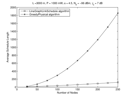
Figure 1: Schedule length vs. number of nodes for LGLS and GP algorithms.

V Conclusions

In this paper, we have proposed a novel scheduling algorithm based on a line graph representation of STDMA network under the physical interference model. Our results demonstrate that the schedule length for the proposed algorithm is substantially lower than that of the GreedyPhysical algorithm. This is due to the fact that we have embedded SINR feasibility conditions into the edge weights of the line graph, and consequently determined a conflict-free schedule.

References

• [1] R.ย Nelson and L.ย Kleinrock, โ€œSpatial TDMA: A Collision-Free Multihop Channel Access Protocol,โ€ IEEE Trans. Commun., vol.ย 33, no.ย 9, pp. 934โ€“944, Sep. 1985.
• [2] P.ย Gupta and P.ย R. Kumar, โ€œThe Capacity of Wireless Networks,โ€ IEEE Trans. Inf. Theory, vol.ย 46, pp. 388โ€“404, Mar. 2000.
• [3] S.ย Ramanathan and E.ย L. Lloyd, โ€œScheduling Algorithms for Multihop Radio Networks,โ€ IEEE/ACM Trans. Netw., vol.ย 1, no.ย 2, pp. 166โ€“177, Apr. 1993.
• [4] W.ย Wang, Y.ย Wang, X.-Y. Li, W.-Z. Song, and O.ย Frieder, โ€œEfficient Interference-Aware TDMA Link Scheduling for Static Wireless Networks,โ€ in Proc. ACM MobiCom, Los Angeles, CA, Sep. 2006, pp. 262โ€“273.
• [5] M.ย Alicherry, R.ย Bhatia, and L.ย Li, โ€œJoint Channel Assignment and Routing for Throughput Optimization in Multi-radio Wireless Mesh Networks,โ€ in Proc. ACM MobiCom, Cologne, Germany, Aug.-Sep. 2005, pp. 58โ€“72.
• [6] G.ย Brar, D.ย M. Blough, and P.ย Santi, โ€œComputationally Efficient Scheduling with the Physical Interference Model for Throughput Improvement in Wireless Mesh Networks,โ€ in Proc. ACM MobiCom, Los Angeles, CA, Sep. 2006, pp. 2โ€“13.
• [7] T.ย Moscibroda and R.ย Wattenhofer, โ€œThe Complexity of Connectivity in Wireless Networks,โ€ in Proc. IEEE Infocom, Barcelona, Spain, Apr. 2006.
• [8] A.ย D. Gore, S.ย Jagabathula, and A.ย Karandikar, โ€œOn High Spatial Reuse Link Scheduling in STDMA Wireless Ad Hoc Networks,โ€ accepted for publication in IEEE Globecom 2007.
• [9] A.ย D. Gore and A.ย Karandikar, โ€œOn High Spatial Reuse Broadcast Scheduling in STDMA Wireless Ad Hoc Networks,โ€ in Proc. National Conference on Communications, Kanpur, India, Jan. 2007, pp. 74โ€“78.
• [10] D.ย B. West, Introduction to Graph Theory, 2ndย ed.ย ย ย Prentice Hall, 2000.
• [11] K.ย Jain, J.ย Padhye, V.ย N. Padmanabhan, and L.ย Qiu, โ€œImpact of Interference on Multi-Hop Wireless Network Performance,โ€ Wireless Networks, vol.ย 11, no.ย 4, pp. 471โ€“487, Jul. 2005.
• [12] M.ย V. Clark, K.ย K. Leung, B.ย McNair, and Z.ย Kostic, โ€œOutdoor IEEE 802.11 Cellular Networks: Radio Link Performance,โ€ in Proc. IEEE ICC, Apr.-May 2002, pp. 512โ€“516.