Entanglement of distant flux qubits mediated by non-classical electromagnetic field

Abstract

The mechanism for entanglement of two flux qubits each interacting with a single mode electromagnetic field is discussed. By performing a Bell state measurements (BSM) on photons we find the two qubits in an entangled state depending on the system parameters. We discuss the results for two initial states and take into consideration the influence of decoherence.

1 Introduction

Entanglement is one of the most fundamental features of quantum mechanics. Besides its fascinating conceptual aspect it also plays an important role in quantum information science because entanglement of qubits is the essential requirement for quantum computing. Various systems have been considered as qubits [1, 2], among them the solid state ones seem to be very promising. In particular superconducting flux qubit has been developed in superconducting ring with Josephson Junction [3, 4]. The junction playing the role of the tunneling barrier can be replaced by a superconducting quantum wire which allows for quantum phase slip [5]. Recently a flux qubit based on semiconducting quantum ring with a controllable barrier has been proposed [6]. In this context the problem of entanglement of two (or more) solid state qubits is of great importance. It has been investigated for superconducting flux qubits interacting via the mutual inductance, via the connecting loop with Josephson Junction and via the LC circuit [7, 8, 9, 4]. It was found [7] that entangled states do not decohere faster than the uncoupled states. This is remarkable considering the expectation that spatially extended entangled states could be very susceptible to decoherence.

In this paper we want to study the entanglement of distant flux qubits by swapping. Presented model considerations may be applied both to superconducting or semiconducting flux qubits. We investigate two independently evolving subsystems each composed of a qubit exposed to a single mode of quantized electromagnetic field (Fig. 1). Contrary to the previous studies where the so called external approximation was used [10] in this paper we take into account the full qubit-field interaction.

The entanglement swapping was originally proposed for photons [11] and has been investigated both theoretically and experimentally [12, 13]. Recently this idea has been used to demonstrate the entanglement of two single atom quantum bits each spontaneously emitting a photon [14]. In our paper we use this idea to entangle solid state qubits which seem to be the most scalable and integrable [15]. The process of entanglement can be described in this case by the interaction Hamiltonian with controllable parameters. The use of solid state qubits instead of atomic qubits described in [14] allows to build systems operating at microwave rather than optical frequencies.

The scheme of entanglement swapping for the discussed system is presented in Fig. 1.

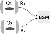
Figure 1: Entanglement swapping scheme

Each qubit $Q$ interacts with an electromagnetic field mode $R$ leading to an entangled qubit-field $(QR)$ state. This effect has been observed in a series of experiments [16]. The two $(QR)_{i}$ ($i=1,2$) systems do not interact with each other and therefore the state of the whole system is a product state. If one then performs the Bell State Measurement (BSM) on $R_{1}$ and $R_{2}$, the partner subsystems $Q_{1}$ and $Q_{2}$ will collapse to an entangled state although they have never physically interacted. To enhance the qubit-field interaction the qubits can be placed into the quantum cavity. The photons can escape from the cavity e.g. through a less reflecting mirror [15, 17]. To quantify the entanglement we calculate the negativity, we discuss the results for two different initial states.
In chapters II-IV we investigate the behaviour at short time scales where the decoherence effects are negligible, the influence of decoherence is studied in chapter V.

2 The qubit-cavity system

To show the idea we consider the rf-SQUID qubit [4] in the presence of static magnetic flux $\phi^{cl}$. The Hamiltonian $H_{Q}$ of such qubit can be written in a pseudo-spin notation

$$H_{Q}=-\frac{1}{2}B_{z}{\sigma_{z}}-\frac{1}{2}B_{x}{\sigma_{x}}.$$ (1)

We operate at $T\ll B_{x}/k_{B}$ in order to neglect thermal fluctuations. The diagonal term $B_{z}$ in (1) has the form

$$B_{z}=2I_{c}\sqrt{6(\beta_{L}-1)}(\frac{\phi_{0}}{2}-\phi)$$ (2)

where $\beta_{L}=2\pi L\left(I_{c}/\phi_{0}\right)>1$,$\phi=\phi^{cl}$, $I_{c}$ is the Josephson junction critical current, $B_{x}$ is the tunneling energy between the two potential wells. Close to $\phi=\frac{1}{2}\phi_{0}$ ($\phi_{0}=h/2e$) the ring is well described by the quantum superpositions of two opposite persistent current states.
At first we describe the process of entanglement of a qubit $Q_{1}$($Q_{2})$ with a single electromagnetic field mode $R_{1}(R_{2})$. We model the electromagnetic field of the resonant cavity as an LC resonator described by $H_{R}$

$$H_{R}=\hbar\omega_{R}\left(a^{\dagger}a+\frac{1}{2}\right).$$ (3)

When the qubit is exposed to the quantized electromagnetic field the total flux $\phi=\phi^{cl}+\phi^{q},$ contains the quantum part

$$\phi^{q}=\sqrt{\frac{\hbar}{2\omega_{R}C_{R}}}\left(a+a^{+}\right)$$ (4)

which leads to the qubit-field coupling. After some algebra we obtain

$$H_{QR} = \frac{\hbar\omega_{Q}}{2}\sigma_{z}+\hbar\omega_{R}\left(a^{\dagger}a+\frac{1}{2}\right)$$ (5)

$$-\hbar\tilde{g}\left(a+a^{\dagger}\right)\left(\sigma_{z}\cos\theta-\sigma_{x}\sin\theta\right)$$

where
$\omega_{Q}$ is the qubit frequency

$$\frac{\hbar\omega_{Q}}{2}=\frac{1}{2}\sqrt{\left(B_{z}^{cl}\right)^{2}+B_{x}^{2}},$$ (6)

the ”mixing angle” $\theta$ [18] is

$$\theta=\tan^{-1}\frac{B_{x}}{B_{z}^{cl}},$$ (7)

and the coupling constant $\tilde{g}$ takes the form

$$\tilde{g}=I_{c}\sqrt{\frac{3\left(\beta_{L}-1\right)}{\hbar\omega_{R}C_{R}}}.$$ (8)

The above considerations can be equally well performed for a semiconducting flux qubit [6] with

$$B_{z}=2I_{0}\left(\frac{\phi_{0}}{2}-\phi^{cl}\right),$$ (9)

where $I_{0}$ is the amplitude of persistent current, $\phi_{0}=h/e,$ $B_{x}$ describes the tunneling amplitude of an electron via a potential barrier.

Assuming realistic values of the parameters for superconducting qubit e.g. $\omega_{R}=2\pi\cdot 50GHz$, $I_{c}=0.5\mu A$, we get $\tilde{g}=0.2\omega_{R}$.

To discuss the qubit-field entanglement we assume that the coherent coupling overwhelms the dissipative processes (strong coupling regime). For creation and manipulation of entangled states, it is thus essential that both the cavity decoherence time $T_{R}$ and the qubit decoherence time $T_{Q}$ are much longer than the qubit-cavity interaction time $T_{\Omega}\sim\pi/\tilde{g}\sim 10^{-11}$ s. Recently a high quality cavities (quality factor $Q_{f}\sim 10^{5}-10^{8}$) have been built [17, 18]. They have a photon storage time $T_{R}$ in the range $0.3\mu s-300\mu s$. The estimated decoherence times $T_{Q}$ of the considered qubits are of the order of a few $\mu s$ (to be specific we assume $T_{Q}\sim 1\mu s$ [4]). In the next two chapters we investigate the system at $t\ll T_{Q},T_{R}$ allowing the entanglement to be obtained before the relaxation processes set in.

3 Entanglement swapping

The $(QR)_{i}$, $i=1,2$ system is described by a state vector $\left|\psi_{QR}(t)\right\rangle_{i}$, which at $t=0$ is a direct product of the qubit and the cavity states:

$$\rho_{(QR)_{i}}(0) = |\psi_{QR}(0)\rangle_{ii}\langle\psi_{QR}(0)|,$$

$$|\psi_{QR}(0)\rangle_{i} = |\sigma n\rangle_{i}=|\sigma\rangle_{i}\otimes|n\rangle_{i},$$ (10)

where $\sigma$ represents the qubit pseudo-spin states ($g$-ground ,$e$-excited), $|n\rangle$ are the photon number eigenstates, forming the so called Fock basis, $n=0,1,2,...$.

The interaction of the qubit with the field leads, in general, to the entangled state

$$|\psi_{QR}\left(t\right)\rangle_{i}=e^{-\frac{i}{\hbar}H_{QR}t}|\psi_{QR}\left(0\right)\rangle_{i}$$ (11)

As the two qubit-boson subsystems do not interact with each other their time evolved state remains separable:

$$\rho\left(t\right)=\rho_{(QR)_{1}}(t)\otimes\rho_{(QR)_{2}}(t)$$ (12)

The time evolution of this composite is a product of two unitary evolutions of its constituents generated by the Hamiltonian (5) where

$$|\psi_{QR}(t)\rangle_{1} = \sum_{n}[a_{n}(t)|gn\rangle_{1}+b_{n}(t)|en\rangle_{1}]$$ (13)

$$|\psi_{QR}(t)\rangle_{2} = \sum_{n}[\tilde{a}_{n}(t)|gn\rangle_{2}+\tilde{b}_{n}(t)|en\rangle_{2}]$$ (14)

The BSM is performed on electromagnetic modes in Fock basis (one photon with the vacuum) [12] and projects the formerly independent qubits onto an entangled state

$$\rho_{QQ}(t)=Tr_{R}\left(|B_{R}^{1}\rangle\langle B_{R}^{1}|\rho(t)\right),$$ (15)

where

$$|B_{R}^{1}\rangle=\frac{1}{\sqrt{2}}\left(|01\rangle-|10\rangle\right)$$ (16)

is one of the Bell states of the electromagnetic field modes, the trace $Tr_{R}$ is taken with respect to photonic degrees of freedom.
After the BSM, the final qubit-qubit ($QQ$) state is of the form

$$\begin{array}[]{rcl}|\psi_{QQ}\rangle&=&[a_{0}(t)\tilde{a}_{1}(t)-a_{1}(t)\tilde{a}_{0}(t)]|gg\rangle\\ &+&[a_{0}(t)\tilde{b}_{1}(t)-a_{1}(t)\tilde{b}_{0}(t)]|ge\rangle\\ &+&[b_{0}(t)\tilde{a}_{1}(t)-b_{1}(t)\tilde{a}_{0}(t)]|eg\rangle\\ &+&[b_{0}(t)\tilde{b}_{1}(t)-b_{1}(t)\tilde{b}_{0}(t)]|ee\rangle\end{array}$$ (17)

We quantify the entanglement by the negativity [19] $N(\rho)=\max(0,-\sum_{i}\lambda_{i})$, where $\lambda_{i}$ are negative eigenvalues of the partially transposed [20] density matrix of the two qubits. For an entangled state, the negativity is positive reaching its maximal value $N=0.5$ for maximally entangled pure state. It vanishes for disentangled states. Moreover, as it is an entanglement monotone it can be used to quantify the degree of entanglement. The use of negativity, instead of some entropic criteria as e.g. linear entropy, allows for simultaneous treatment of the entanglement of pure and mixed states. Let us notice that in general (e.g. beyond Jaynes–Cummings approximation) the qubit–resonator system evolves in an infinite dimensional Hilbert space. It is known [21] that in high dimensional systems the so called PPT (positive with respect to partial transposition) entangled states can occur. They cannot be detected by the Peres criterion and negativity. In this paper we limit our attention to the NPT entangled states i.e those which are negative with respect to partial transposition.

4 Numerical results

We present results for entanglement of both qubit-field ($N_{i}$) and qubit-qubit ($N_{QQ}$) systems. As the calculations are numerical we are not limited to the weak coupling regime. In numerical calculations the Hilbert space of microwave modes is truncated at $n_{\max}=10$. We test the validity of the truncation by controlling the traces of the matrices [22] being never smaller than $0.99$.

There are many parameters affecting entanglement of qubits. To show the idea we restrict our considerations to selected examples and discuss the results for two initial states. In our model calculation we assume that both qubits are identical, the analysis can easily be extended beyond . In this paper we consider only the resonant case i.e. $\omega_{R_{i}}=\omega_{Q_{i}}\equiv\omega_{R}=2\pi\cdot 50GHz$. The values of $\tilde{g}_{i}$ are in the units of $\omega_{R}$.

At first we assume the initial state to be

$$|\psi_{QR}(0)\rangle_{1}\otimes|\psi_{QR}(0)\rangle_{2}=|e0\rangle_{1}\otimes|g1\rangle_{2}.$$ (18)

In Fig. 2 we show how the qubit-field negativity depends on the coupling strength $\tilde{g}$ and in Fig. 3 its behaviour for different values of the mixing angle $\theta$.

Figure 2: The qubit-field negativity for different values of $\tilde{g}$, $\theta=\pi/2$, initial state $|e0\rangle$ and $\omega_{Q}=\omega_{R}=2\pi\cdot 50GHz$.

Figure 3: The qubit-field negativity for different values of $\theta$, $\tilde{g}=0.2$, initial state $|e0\rangle$, $\omega_{Q}=\omega_{R}=2\pi\cdot 50GHz$.

Comparing these figures we see that both $\theta$ and $\tilde{g}$ influence the effective qubit-field interaction strength. The increase of $\tilde{g}$ causes the increase of the Rabi oscillation frequency and the entanglement arises faster than for weaker coupling. Similarly, bringing $\theta$ closer to $\pi/2$ increases the Rabi frequency. For $\theta=0$ the $QR$ entanglement disappears. In the following we assume $\theta=\pi/2$ which gives the strongest effective coupling with fixed $\tilde{g}$.

Figure 4: Negativities $N_{1}$ (crosses), $N_{2}$ (dashed line), $N_{QQ}$ (solid line) and probabilities for finding the two qubits in different states after the BSM. The initial state $|e0\rangle_{1}\otimes|g1\rangle_{2}$, coupling strength $\tilde{g}_{i}=0.2$, $\theta_{i}=\pi/2$.

In the upper panel of Fig. 4 the oscillating qubit-field negativities $N_{1}$ and $N_{2}$ reflect the varying degree of entanglement as a function of time. The differences in these two curves arise from different initial states for $(QR)_{i}$ systems ( $|e0\rangle_{1}\otimes|g1\rangle_{2}$). If we perform the BSM at certain time $t$ we obtain an entanglement of qubits (solid line) conditioned by the degree of entanglement of ($QR)_{i}$. In particular if we do the BSM at the time window in which the $(QR)_{i}$ subsystems are almost maximally entangled we obtain the maximally entangled qubits with $N_{QQ}\sim 0.5$. On the other hand if we perform the BSM in the time window where the $(QR)_{i}$ subsystems are weakly entangled the $QQ$ entanglement is vanishingly small.

We emphasize that the ’time’ in the figures is either the physical time of the quantum evolution of the $QR$ system or the time, called the ’BSM time’, at which the BSM was performed.

The bottom parts of Fig. 4 and Fig. 5 show the probabilities of finding the qubits in $|ee\rangle$, $|eg\rangle$, $|ge\rangle$ and $|gg\rangle$ states (e.g. $P_{eg}=|\langle eg|\psi_{QQ}(t)\rangle|^{2}$). We see that the final state belongs to the subspace spanned by $|eg\rangle$ and $|ge\rangle$. This is because of the value of $\theta_{i}=\pi/2$ and the chosen projection operator. For such $\theta$ the interaction term in (5) reduces to the form $\tilde{g}\left(a^{\dagger}+a\right)\sigma_{x}$ that excites only $|en\rangle$ with $n$ even and $|gm\rangle$ with $m$ odd if we start from $|e0\rangle$ and $|g1\rangle$ initial states respectively. Then when the BSM is done the only nonzero elements, in equation (17), are $b_{1}\tilde{a}_{0}$ and $a_{1}\tilde{b}_{0}$. The relation between the ’occupation probabilities’ can be directly translated into the entanglement of the state: the more one of the probabilities dominates the other the less entangled is the state and when the probabilities $P_{eg}$ and $P_{ge}$ equal 0.5 the entanglement reaches its maximal value.

The decay rate of the $QR$ system can be estimated as [18]

$$\frac{1}{T_{QR}}=\frac{1}{2}\left(\frac{1}{T_{Q}}+\frac{1}{T_{R}}\right)$$ (19)

Assuming the cavity with $Q_{f}=10^{5}$ we find $T_{R}\sim 0.3\mu s$ and $T_{QR}\sim 0.5\mu s$. For the cavity with $Q_{f}=10^{6}$ we get $T_{R}\sim 3\mu s$ and $T_{QR}\sim 1.5\mu s$. The decoherence time of the $QQ$ entangled state is accordingly $T_{QQ}\sim T_{Q}\sim 1\mu s$. This estimation is in agreement with the experimental findings [7] that entangled states do not decohere faster than uncoupled systems.

Figure 5: $N_{1}$ (crosses), $N_{2}$ (dashed line) and $N_{QQ}$ (solid line) negativities (top) and probabilities (bottom) for the initial state (20), $\theta_{i}=\pi/2$ and small detuning $\tilde{g_{1}}=0.2,~{}\tilde{g_{2}}=0.202$.

For the initial state

$$|\psi_{QR}(0)\rangle_{1}\otimes|\psi_{QR}(0)\rangle_{2}=|e0\rangle_{1}\otimes|e0\rangle_{2}$$ (20)

the situation looks different. The identity of the systems (the same parameters and initial states) leads to the striking results. Whenever we perform the BSM we almost always (with some exceptions) obtain the maximally entangled qubit-qubit state. In order to show some subtleties we take the systems slightly detuned with $\tilde{g_{1}}=0.2,\tilde{g_{2}}=0.202$ and treat $\tilde{g_{1}}=\tilde{g_{2}}=0.2$ as a limiting case. Because the two $QR$ systems are almost identical differing minutely in Rabi frequencies, they evolve to almost the same quantum states and even if $QR$’s are not strongly entangled the BSM gives nearly the same probabilities $P_{eg}=P_{ge}\sim 0.5$. In consequence, we get almost maximally entangled $QQ$ state for arbitrary BSM time, except for some moments (in Fig. 5 for $\omega_{R}t\sim 16$ ) at which the norm of the BSM output approaches zero and the above quantities become undefined. If the BSM were performed at these moments the entanglement would be unsuccessful. In the case $\tilde{g_{1}}=\tilde{g_{2}}$ the probabilities are always the same and the qubits get maximally entangled for each BSM time (see B line in Fig. 7) with the exceptions described above. Similar results we have obtained for the initial state $|g1\rangle_{1}\otimes|g1\rangle_{2}$.

5 Decoherence

Design and construction of quantum devices is always limited by the influence of environment. Here, instead of rigorous treatment, developed e.g. for pure dephasing [23, 24], we apply the commonly used Markovian approximation [25] and model the reduced dynamics of the $QR$ system in terms of master equation generating complete positive dynamics [26]. Following [18] we assume that the effect of environment can be included in terms of two independent Lindblad terms:

$$\dot{\rho}(t)=[L_{H}-\frac{1}{2}L_{1}-\frac{1}{2}L_{2}]\rho(t)$$ (21)

where the ’conservative part’ is given by

$$L_{H}(\cdot)=-i[H_{Q},\cdot]$$ (22)

whereas the ’Lindblad dissipators’

$$L_{k}(\cdot)=A^{\dagger}_{k}A_{k}(\cdot)+(\cdot)A^{\dagger}_{k}A_{k}-2A_{k}(\cdot)A^{\dagger}_{k},\,\,\,\,k=1,2.$$ (23)

are expressed in terms of creation and annihilation operators ’weighted’ by suitable lifetimes $A_{1}=a/\sqrt{T_{R}}$ and $A_{2}=\sigma_{-}/\sqrt{T_{Q}}$. To be precise we assume $T_{Q}\sim 1\mu s$, $T_{R}\sim 0.3\mu s$. As the dynamics becomes non-unitary the system evolves, in general, to the mixed state. The BSM applied to the density operator of the mixed states is well defined physical operation of projection and reduction which can be shown to be completely positive (see Appendix) and thus applicable to arbitrary ${\rho}$.

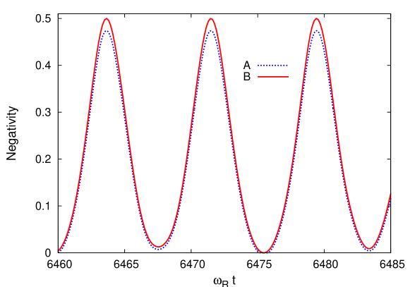
Figure 6: (color online) The QQ negativity with (A) and without (B) decoherence for the initial state (18). The parameters are $\theta_{i}=\pi/2$, $\tilde{g}_{i}=0.2$, $T_{R_{i}}=0.3\mu s$, $T_{Q_{i}}=1\mu s$.

In Fig. 6 we show the results of the master equation simulations of the negativity (the line labeled by A in Fig. 6) in comparison with the calculations which neglect decoherence (the line labeled by B) for the initial state (18). The periodicity with the decoherence included is conserved. For better visibility we present the results only in a short time period. We see that decoherence decreases slightly the amplitude of the oscillations.
The influence of decoherence on the entanglement of the system starting from (20) (Fig. 7) is much more dramatic. In contrast to the non dissipative case (B) the result of the BSM depends strongly on the BSM time and the character of the entanglement becomes quasi-periodic.

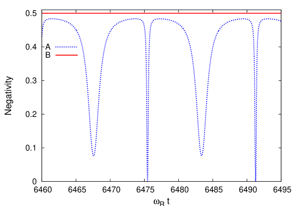
Figure 7: (color online) The QQ negativity with (A) and without (B) decoherence for the initial state (20). The parameters are as in Fig. 6.

In Fig. 8. we show the decrease of the amplitude of negativity as a function of time in the larger time scale for both initial conditions. The decrease is faster for the initial state (18) in comparison with that for the initial state (20).

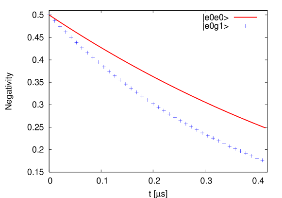
Figure 8: (color online) The amplitude of the qubit-qubit negativity plotted as a function of BSM time for two different initial states. The parameters are as in Fig. 6.

6 Conclusions

We investigated a mechanism for creation of entanglement of two qubits, each interacting with a single mode electromagnetic field coming from independent sources. This interaction leads to two independent entangled qubit-field states and that BSM performed on the electromagnetic field modes projects the qubits onto an entangled state. Thus we discussed transfer of quantum information between systems having different physical nature and defined in Hilbert spaces of different dimensions.

In the first part of the paper we have dealt with the pure states which is justified to some extent by estimated relatively long decoherence times. The discussed systems offer the advantage of reaching a strong coupling regime between light and matter. We have checked that the Jaynes-Cummings model, valid for weaker $QR$ coupling [27], gives the results in agreement with our calculations for $g\leq 0.03\omega_{R}$. Assuming reasonable values of parameters we found that the strong coupling regime ($T_{\Omega}^{-1}\gg T_{R}^{-1},T_{Q}^{-1}$) can be realized and coherent manipulations of qubits (especially with the quantum error correction technique) and maximally entangled qubit-qubit states are possible.
Analyzing the dynamics of the system in the presence of decoherence we found that the observation of coherent phenomena and in particular the generation of highly entangled states is still possible.

It seems that entanglement of distant qubits by swapping can have some advantages over standard schemes of setting up entanglement that rely on generating entangled subsystems at a point and supplying them to distant areas. The qubits emerge entangled despite the fact that they never interacted in the past and therefore they do not influence each other by disturbing the single qubit features. They can be at much larger distances as the scheme does not depend essentially on the distance between them. The degree of entanglement depends on the moment at which the BSM was performed. Verifying experimentally that two qubits are unambiguously entangled is a difficult task requiring sophisticated methods such as e.g. quantum state tomography [28]. The solid state qubits and their entanglement discussed in this paper can be scaled to a larger set of quantum bits [29]. It can be of interest in the study of fundamental laws of quantum mechanics and can be useful in quantum information processing and quantum communication. It seems that the experimental realization of the presented model considerations may be performed with currently available technologies. Following [21], we hope that ’what is predicted by quantum formalism must occur in the laboratory’. Sooner or later.

Appendix

We will prove that the transformation described by (15) and (16) which was defined for pure states, makes sense also for an arbitrary mixed state of the two-qubit-field ($QRQR$) system, ie. it is described by a completely positive operator transforming an arbitrary density matrix of the full system into a density matrix of two-qubit ($QQ$) system. Although it is easy to understand on a purely physical basis (transformation consists of a measurement and a reduction to a subsystem), it is instructive to give an explicit proof of the statement. As a bonus we will easily find an explicit Kraus form of the transformation in question.

Let

$$\rho=\sum_{\begin{subarray}{c}\mu k\nu l\\ \varsigma m\tau n\end{subarray}}\rho^{\mu k\nu l}_{\varsigma m\tau n}|\mu k\nu l\rangle\!\langle\varsigma m\tau n|,$$ (24)

where, cf. (3),

$$|\,\mu k\nu l\rangle=|\,\mu\rangle_{1}\otimes|\,k\rangle_{1}\otimes|\,\nu\rangle_{2}\otimes|\,l\rangle_{2}=|\,\psi_{QR}\rangle_{1}\otimes|\,\psi_{QR}\rangle_{2}$$ (25)

for $\mu,\nu\in\{g,e\}$, $k,l\in\{0,1,\ldots\}$ form a basis of pure states for the full system.

For the moment let us consider only the Jaynes-Cummings approximation where we take into account only the modes $|\,0\rangle$ and $|\,1\rangle$ of the electromagnetic field, hence all Latin indices in (24) and (25) take the values $0,1$ only. In this case density matrices of the $QRQR$ system act in the $16$-dimensional complex space, $\mathcal{H}_{1}=\mathbb{C}^{16}$, and as such form a subset of the $16\times 16$-dimensional complex linear space. Analogously, density matrices of the $QQ$ system, acting in the $4$-dimensional complex space, $\mathcal{H}_{2}=\mathbb{C}^{4}$, form a subset of the $4\times 4$-complex space. The transformation (denoted in the following by $\Lambda$) described by (15) regarded on the whole $256$-dimensional complex space transforms it into the $16$-dimensional one. Straightforward calculations give

$$\Lambda(\rho) =: \sigma=\sum_{\begin{subarray}{c}\mu,\nu\in\{g,e\}\\ \varsigma,\tau\in\{g,e\}\end{subarray}}\sigma^{\mu\nu}_{\varsigma\tau}|\mu\nu\rangle\!\langle\varsigma\tau|,$$ (26)

$$\sigma^{\mu\nu}_{\varsigma\tau} = \frac{1}{2}\left(\rho^{\mu 0\nu 1}_{\varsigma 0\tau 1}-\rho^{\mu 1\nu 0}_{\varsigma 0\tau 1}-\rho^{\mu 0\nu 1}_{\varsigma 1\tau 0}+\rho^{\mu 1\nu 0}_{\varsigma 1\tau 0}\right),$$ (27)

where $|\,\mu\nu\rangle:=|\,\mu\rangle_{1}\otimes|\,\nu\rangle_{2}$ form a basis of pure states of the $QQ$ system. In the following we will need only

$$\Lambda\big{(}|\mu k\nu l\rangle\!\langle\varsigma m\tau n|\big{)}=$$ (28)

$$= \frac{1}{2}\big{(}\delta_{0k}\delta_{1l}\delta_{0m}\delta_{1n}-\delta_{1k}\delta_{0l}\delta_{0m}\delta_{1n}$$

$$- \delta_{0k}\delta_{1l}\delta_{1m}\delta_{0n}+\delta_{1k}\delta_{0l}\delta_{1m}\delta_{0n}\big{)}|\mu\nu\rangle\!\langle\varsigma\tau|$$

To check the complete positivity of $\Lambda$ we use the Choi-Jamiolkowski isomorphism defined as [30]

$$\mathcal{J}(\Lambda)=(\Lambda\otimes\mathbb{I}_{1})(P_{+}),$$ (29)

where $\mathbb{I}_{1}$ is the identity operator on the $256$-dimensional space and $P_{+}$ is a maximally entangled state on the $\mathcal{H}_{1}\otimes\mathcal{H}_{1}$ space

$$P_{+}=|\Phi_{+}\rangle\!\langle\Phi_{+}|,\quad|\,\Phi_{+}\rangle=\sum\limits_{\mu k\nu l}|\,\mu k\nu l\rangle\otimes|\,\mu k\nu l\rangle.$$ (30)

According to the Choi theorem [31], $\Lambda$ is completely positive if and only if $\mathcal{J}(\Lambda)$ is a positive-definite operator. Applying (29) and (28) to (30) we get

$$\mathcal{J}(\Lambda)=|\Phi\rangle\!\langle\Phi|,$$ (31)

where

$$|\,\Phi\rangle=\frac{1}{\sqrt{2}}\sum\limits_{\mu\nu}|\,\mu\nu\rangle\otimes\big{(}|\,\mu 0\nu 1\rangle-|\,\mu 1\nu 0\rangle\big{)}.$$ (32)

article Hence $\mathcal{J}(\Lambda)$ is a projection and as such a positive definite operator, consequently $\Lambda$ is completely positive.

The obtained results allow to write explicitly the so called Kraus form of $\Lambda$,

$$\Lambda(\rho)=\sum_{n}A_{n}\rho A_{n}^{\dagger},$$ (33)

where $A_{n}$ are $\mathrm{dim}\mathcal{H}_{2}\times\mathrm{dim}\mathcal{H}_{1}=4\times 16$ matrices. To this end [32] we have to perform the spectral decomposition of the positive definite operator $\mathcal{J}(\Lambda)$

$$\mathcal{J}(\Lambda)=\sum\limits_{\mu}d_{n}|\chi^{\prime}_{n}\rangle\!\langle\chi^{\prime}_{n}|.$$ (34)

Since $d_{n}$ are positive, we can rescale the eigenvectors

$$|\,\chi_{n}\rangle:=\sqrt{d_{n}}|\,\chi^{\prime}_{n}\rangle.$$ (35)

Now the operators $A_{n}$ can be found in the form

$$A_{n}:=\big{(}\mathbb{I}_{2}\otimes\langle\Phi_{+}|\big{)}\big{(}|\,\chi_{n}\rangle\otimes\mathbb{I}_{1}\big{)},$$ (36)

where $\mathbb{I}_{2}$ is the identity on $\mathcal{H}_{2}$. The above formula should be properly understood. Observe that since $|\,\chi_{n}\rangle$ is an element of $\mathcal{H}_{2}\otimes\mathcal{H}_{1}$, it has the form $|\,\chi_{n}\rangle=\sum_{i}|\,\phi_{n,i}\rangle\otimes|\,\xi_{n,i}\rangle$, where $|\,\phi_{n,i}\rangle\in\mathcal{H}_{2}$, $|\,\xi_{n,i}\rangle\in\mathcal{H}_{1}$, whereas $\langle\Phi_{+}|=\sum\langle\mu k\nu l|\otimes\langle\mu k\nu l|$. Hence

$$A_{n} = \big{(}\mathbb{I}_{2}\otimes\langle\Phi_{+}|\big{)}\left(|\,\chi_{n}\rangle\otimes\mathbb{I}_{1}\right)$$ (37)

$$= \big{(}\mathbb{I}_{2}\otimes\sum_{\mu k\nu l}\langle{\mu k\nu l}|\otimes\langle{\mu k\nu l}|\big{)}\big{(}\sum_{i}|\,\phi_{n,i}\rangle\otimes|\,\xi_{n,i}\rangle\otimes\mathbb{I}_{1}\big{)}$$

$$= \sum_{i,{\mu k\nu l}}\langle{\mu k\nu l}|\xi_{n,i}\rangle\,|\phi_{n,i}\rangle\!\langle{\mu k\nu l}|.$$

In our case $\mathcal{J}(\Lambda)$ has only one non vanishing eigenvalue corresponding to the eigenvector $|\,\chi_{1}\rangle=|\,\Phi\rangle=\sum_{\mu\nu}|\,\phi_{1,\mu\nu}\rangle\otimes|\,\xi_{1,\mu\nu}\rangle$. Hence $|\,\phi_{1,\mu\nu}\rangle=|\,\mu\nu\rangle$ and $|\,\xi_{1,\mu\nu}\rangle=\big{(}|\,\mu 0\nu 1\rangle-|\,\mu 1\nu 0\rangle\big{)}/\sqrt{2}$. Using (32) and (37) we obtain finally:

$$A=\frac{1}{\sqrt{2}}\sum_{\mu\nu}\big{(}|\mu\nu\rangle\!\langle\mu 0\nu 1|-|\mu\nu\rangle\!\langle\mu 1\nu 0|\big{)}$$ (38)

A short calculation shows that indeed, cf. (26),

$$\Lambda(\rho)=A\rho A^{\dagger}.$$ (39)

The calculations do not change considerably if we go beyond the Jaynes-Cummings approximation, by taking into account arbitrary finite numbers of photons in each cavity. In fact, in this case, the only difference consists of extending all summations over the number of photons from two terms corresponding to 0 and 1 to the desired numbers of cavity excitations which we would like to regard. The final results (38) and (39) remain unaltered. The situation is more subtle if we want to take into account the infinite number of possible photonic excitations of the cavity modes. The corresponding cavity Hilbert space becomes now infinite-dimensional and a straightforward generalization of the Choi-Jamiołkowski isomorphism does not exist – one has to resort to slightly more involved procedures to investigate directly the complete positivity [33]. It is, however, not really needed in our case. As it is easy to check, the final result (38), (39) is correct also in the infinite-dimensional setting.

References

References

- [1] J M Raimond, M Brune, S Haroche 2001 Rev. Mod. Phys. 73, 565
- [2] Y Nakamura, Yu A Pashkin, J S Tsai 1999 Nature 398 786
- [3] J E Mooij, T P Orlando, L S Levitov, L Tian, C H van der Wal, S Lloyd 1999 Science 285, 1036
- [4] R Migliore, A Messina 2003 Phys. Rev. B 67, 134505; R Migliore, A Messina 2005 Phys. Rev. B 72, 214508
- [5] J E Mooij, C J P Harmans 2005 New J. Phys. 7, 219
- [6] E Zipper, M Kurpas, M Szelag, J Dajka, M Szopa 2006 Phys. Rev. B 74, 125426
- [7] A J Berkeley at al. 2003 Science 300, 5625; R McDermott et al. 2005 Science 307, 1299
- [8] B L T Plourde et al. 2004 Phys. Rev. B 70, 140501; A Izmalkov et al. 2004 Phys. Rev. Lett. 93, 037003
- [9] M Paternostro, G Falci, M Kim. G M Palma 2004 Phys. Rev. B 69, 214502
- [10] J Dajka, M Szopa, A Vourdas, E Zipper 2004 Phys. Rev. B 69, 043505; J Dajka, A Vourdas, S Zhang, and E Zipper 2006 J. Phys. Cond. Matter 18, 4, 1376
- [11] M Zukowski, A Zeilinger, M A Horne, A K Ekert 1993 Phys. Rev. Lett. 71, 4287
- [12] H. de Riedmatten, I. Markicic, J. A. W. van Houwelingen, W. Tittel, H. Zbinden, N. Gisin 2005 Phys. Rev. A 71, 050302
- [13] J-W Pan et al. 1998 Pys. Rev. Lett. 80, 3891; J-W Pan et al. 2001 Phys. Rev. Lett. 86, 4435 ; F.Sciarrino, E Lombardi, G Milani, F De Martini 2002 Phys.Rev. A 66, 024309
- [14] D L Moehring, P Maunz, S Olmschenk, K C Younge, D N Matsukevich, L-M Duan, C Monroe 2007 Nature 449, 68
- [15] S D Barrett, P Kok 2005 Phys. Rev. A71, 060310(R)
- [16] I Chiorescu et al. 2004 Nature 431, 159; A Walraff et al. 2004 Nature 431, 162
- [17] J M Raimond, M Brune, S Haroche 2001 Rev. Mod. Phys. 73, 565
- [18] A Blais, R Huang, A Wallraff, S M Girvin, R J Schoelkopf 2004 Phys. Rev. A 69, 062320.
- [19] G Vidal, R F Werner 2002 Phys. Rev. A 65, 032314
- [20] A Peres 1996 Phys. Rev. Lett. 77, 1413
- [21] R Horodecki, P Horodecki, M Horodecki, K Horodecki 2007 quant-ph/0702225v2
- [22] R Migliore, A Konstadopoulou, A Vourdas, T P Spiller, A Messina 2003 Phys. Lett. A 319, 67
- [23] Łuczka J 1990 Physica A 167, 919
- [24] J Dajka, M Mierzejewski, J Łuczka 2007 J. Phys. A: Math. Theor. 40 F879
- [25] C W Gadiner, P Zoller 2000 Quantum noise, Springer, Berlin
- [26] R Alicki, K Lendi 1987 Quantum dynamical semigroups and applications, (Lecture Notes in Physics 286), Berlin, Springer
- [27] A T Sornborger, A N Cleland, M R Geller 2004 Phys. Rev. A 70, 052315
- [28] M Steffen et al. 2006 Science 313, 1423
- [29] S Bose, V Vedral, P L Knight 1998 Phys. Rev. A 57, 822
- [30] A. Jamiolkowski 1972 Rep. Math. Phys. 3 275278.
- [31] M D Choi 1975 Lin Alg. Appl. 10285290.
- [32] P Arrighi and C Patricot 2004 Ann. Phys. 311 2652.
- [33] J Grabowski, M Kuś and G Marmo 2007 Open Sys. Information Dyn. 14 355.