HFAG Charm Mixing Averages

Abstract

Recently the first evidence for charm mixing has been reported by several experiments. To provide averages of these mixing results and other charm results, a new subgroup of the Heavy Flavor Averaging Group has been formed. We here report on the method and results of averaging the charm mixing results.

I Introduction

Almost since the discovery of charm mesons, mixing of $D^{0}-\overline{D}^{0}$ mesons have been sought in analogy to the well-known $K^{0}-\overline{K}^{0}$ mixing. Due to very effective GIM suppression, the expected mixing rate in the charm system is much smaller than for kaons. Only very recently, the BaBar Aubert:2007wf and Belle Staric:2007dt collaborations have reported the first evidence of charm mixing. These results have renewed the interest from the theory community as the observed mixing rate could be caused by physics beyond the standard model or at least provide additional constraints on new physics.

None of the mixing measurement have a significance above four standard deviations, but several have similar precision for the mixing parameters. By combining the measurements we therefore obtain more precise values for the mixing parameters and exclude the no-mixing hypothesis with larger confidence. Combining the different mixing measurements is not completely straightforward, since not all measurements are sensitive to the same charm mixing parameters.

The Heavy Flavor Averaging Group (HFAG) in 2006 created a subgroup with the responsibility of providing averages of charm physics measurements. One of the high priority tasks of this group is to combine the charm mixing measurements into world-average values for the fundamental mixing parameters. The first average assuming CP conservation was shown at FPCP Schwartz:2007fw . Besides those results, we here report the first results of combining mixing measurements where we allow for CP violation.

II Averaging Method

Mixing is present in the $D^{0}-\overline{D}^{0}$ system if the mass eigenstates, $|D_{1}\rangle$ and $|D_{2}\rangle$, differ from the flavor eigenstates, $|D^{0}\rangle$ and $|\overline{D}^{0}\rangle$. Generally one can write $|D_{1,2}\rangle=p|D^{0}\rangle\pm q|\overline{D}^{0}\rangle$. The variables of fundamental interest are the mass difference, $\Delta M=M_{1}-M_{2}$ and decay width difference, $\Delta\Gamma=\Gamma_{1}-\Gamma_{2}$ between the two mass eigenstates. Traditionally, in charm mixing one uses the dimensionless variables, $x=\Delta M/\Gamma$ and $y=\Delta\Gamma/2\Gamma$, where $\Gamma$ is the average decay width. CP violation in mixing or in the interference between mixing and decay would manifest itself as $|q/p|\neq 1$ and $\phi=\arg(q/p)\neq 0$, respectively. In addition CP violation could show up in the decay itself giving rise to decay mode dependent parameters.

Most measurements do not directly measure $(x,y)$. For instance in mixing measurements using $D^{0}\rightarrow K^{+}\pi^{-}$ decays there is a unknown strong phase, $\delta_{K\pi}$, so the results obtained are for $x^{\prime}=x\cos\delta_{K\pi}+y\sin\delta_{K\pi}$ and $y^{\prime}=-x\sin\delta_{K\pi}+y\cos\delta_{K\pi}$. In the averaging procedure, we first combine measurements of the same parameters to obtain the more precise observables. Most measurements are performed using likelihood fits and the combination is therefore performed by multiplying likelihood functions from each measurement and finding the new maximum. By combining likelihoods, correlations between observables and possible non-Gaussian tails are taken into account. For measurements which are not using likelihoods, we construct a likelihood using symmetrized, Gaussian uncertainties. To combine different types of measurements, the different combined likelihoods are recalculated as a function of $(x,y,\delta_{K\pi})$ minimizing over any other variables. $\delta_{K\pi}$ is included since there is both a direct measurement Asner:2006md and by combining the $D^{0}\rightarrow K^{+}\pi^{-}$ measurement with the other measurement of $x$ and $y$, one can also get a precise measurement of $\delta_{K\pi}$. When plotting confidence contours for $(x,y)$ we minimize the likelihood over $\delta_{K\pi}$.

The combining of likelihood functions is currently only done for the CP conserving case. In principle it can be done also for the CP violating case by simply having two more variables, $|q/p|$ and $\phi$, in the final likelihood function. Unfortunately not all likelihoods are currently available for the measurements which allow for CP violation. A simple combination is therefore performed by forming a $\chi^{2}$ of all measurements expressed in terms of the fundamental mixing parameters. The $\chi^{2}$ assumes Gaussian errors, but correlations between observables in each individual measurement is taken account by using the full covariance matrix for each result.

III CP Conserving Averages

The following averages were performed by adding log likelihoods from fits where CP conservation was assumed.

III.1 Lifetime Ratio Average

One can observe charm mixing by finding a difference in the lifetime measured in decays to CP eigen states such as $D^{0}\rightarrow K^{+}K^{-}$ and $D^{0}\rightarrow\pi^{+}\pi^{-}$ and the mixed-CP decay $D^{0}\rightarrow\pi^{+}K^{-}$. We combine six results Staric:2007dt ; Aitala:1999dt ; Link:2000cu ; Csorna:2001ww ; Aubert:2003pz ; Abe:2001ed from such analyzes. All of these measure $y_{\mathrm{CP}}=\tau_{K\pi}/\tau_{hh}-1$. In the limit of CP conservation one has $y_{\mathrm{CP}}=y$. The average of the six measurements is $y_{\mathrm{CP}}=(1.12\pm 0.32)\times 10^{-2}$. This is $3.5\sigma$ from the no-mixing hypothesis. As can be seen from Figure 1, this average is mainly driven by the recent Belle measurement.

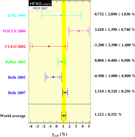
Figure 1: Measured $y_{\mathrm{CP}}$ values and the HFAG average.

III.2 Mixing Rate Average

Wrong-signed semileptonic decays provide a clean way of searching for charm mixing, but the measurements are only sensitive to the integrated mixing rate $R_{M}=(x^{2}+y^{2})/2$. Four measurements Aitala:1996vz ; Cawlfield:2005ze ; Abe:2005nq ; Aubert:2007aa are combined and give an average of $R_{M}=(1.7\pm 3.9)\times 10^{-4}$. In addition to the semileptonic decays, $R_{M}$ can also measured in the analysis of fully hadronic decays. The semileptonic result is therefore combined from two hadronic analyzes Aubert:2006kt ; Aubert:2006rz and in addition an analysis of tagged decays at the $\psi(3770)$ Asner:2006md . The combination is illustrated in Figure 2 and gives an average value of $R_{M}=(2.1\pm 1.1)^{-4}$. In the transformation to a likelihood in $(x,y)$, we ignore the non-physical region of $R_{M}<0$.

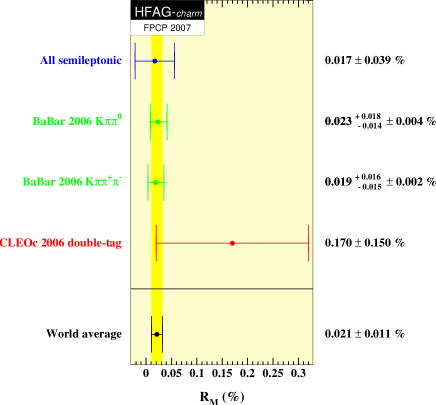
Figure 2: The mixing rate from measurements using semileptonic $D^{0}$ decays are averaged with results from multi-body hadronic charm decays.

III.3 $(x,y)$ Average

One can measure $x$ and $y$ directly using a time-dependent Dalitz plot analysis of $D^{0}\rightarrow K_{S}^{0}\pi^{+}\pi^{-}$ decays. Two measurements Asner:2005sz ; Zhang:2007dt have been published and these have been averaged by HFAG and gives $x=(8.1\pm 3.3)\times 10^{-3}$ and $y=(3.1\pm 2.8)\times 10^{-3}$. Combining this average with the averages above for $R_{M}$ and $y_{\mathrm{CP}}$ using likelihoods mapped as a function of $(x,y)$ we obtain $x=(9.2\pm 3.4)\times 10^{-3}$ and $y=(7.0\pm 2.2)\times 10^{-3}$. Contours of the combined likelihood function at the levels corresponding to $1$ to $5\sigma$ confidence levels are shown in Figure 3. Note that the confidence levels shown correspond to two-dimensional coverage probabilities of 68.27%, 95.45%, etc., and therefore $2\Delta\ln L=2.30,6.18,$ etc.

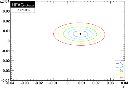
Figure 3: Confidence level contours in the mixing parameters $(x,y)$ from the combination of $y_{\mathrm{CP}}$, $R_{M}$ and $(x,y)$ from the time-dependent Dalitz analysis of $D^{0}\rightarrow K_{S}\pi^{+}\pi^{-}$.

III.4 Averages for $D^{0}\rightarrow K^{+}\pi^{-}$ Decays

As mentioned above, one can measure $x^{\prime}$ and $y^{\prime}$ using the doubly-Cabibbo suppressed (DCS) decay $D^{0}\rightarrow K^{+}\pi^{-}$. The likelihood functions are available for two measurements Aubert:2007wf ; Zhang:2006dp of this type. These are combined and gives the averages $x^{\prime 2}=(-0.1\pm 2.0)\times 10^{-4}$ and $y^{\prime}=(5.5^{+2.8}_{-3.7})\times 10^{-3}$. The corresponding likelihood contours are shown in Figure 4.

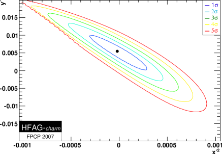
Figure 4: Confidence level contours from the combination of BaBar and Belle measurements using $D^{0}\rightarrow K^{+}\pi^{-}$. The wiggles in the 4 and $5\sigma$ contours for $x^{\prime 2}<0$ is a binning effect.

III.5 World Average

The combined likelihood for $D^{0}\rightarrow K^{+}\pi^{-}$ decays can be expressed as a function of $(x,y,\delta_{K\pi})$ ignoring the part with $x^{\prime 2}<0$. This likelihood can be combined with the likelihood from the combination of the other mixing results in Section III.3 which do not depend on $\delta_{K\pi}$. An additional constraint comes from a CLEO-c measurement Asner:2006md of $\cos\delta_{K\pi}=1.09\pm 0.66$, where a small dependence on $x$ and $y$ is ignored in the combination. Figure 5 shows the likelihood contours in $(x,y)$ after minimizing over $\delta_{K\pi}$. The region around the central value is almost unchanged with respect to the result without the $D^{0}\rightarrow K^{+}\pi^{-}$ decays (Figure 3). This is also reflected in the over all average for $x$ and $y$ which are

$$x = (8.7^{+3.0}_{-3.4})\times 10^{-3},$$

$$y = (6.6\pm 2.1)\times 10^{-3}.$$

The $D^{0}\rightarrow K^{+}\pi^{-}$ measurements do not contribute much to the central value, because of the poorly known phase $\delta_{K\pi}$. However they do help exclude the no-mixing hypothesis and cause the dip seen in the contours close to $(x,y)=(0,0)$. At $(x,y)=(0,0)$ we obtain $2\Delta\ln L=37$ with respect to the minimum. This corresponds to a significance of the combined mixing signal of $5.7\sigma$.

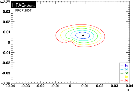
Figure 5: Confidence level contours from combining all mixing measurements under the assumption of CP conservation.

The combination also gives an improved value for $\delta_{K\pi}$. This can be seen in the projection of the likelihood after minimizing over $x$ and $y$ in Figure 6. The combination gives $\delta_{K\pi}(=0.33^{+0.26}_{-0.29})\mathrm{rad}$. Without the CLEO-c measurement of $\delta_{K\pi}$, there would be an equally good second minimum at $\delta_{K\pi}=-2.17\mathrm{rad}$.

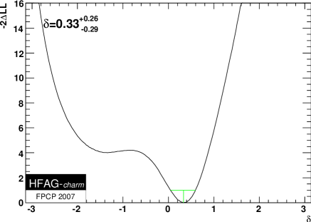
Figure 6: Log-likelihood function for the strong phase, $\delta_{K\pi}$, from combining all mixing measurements.

IV CP Violating Averages

Measurements of charm mixing can be done without assuming CP conservation by fitting $D^{0}$ and $\overline{D}^{0}$ mesons as separate samples. Most of the measurements above have done that and we therefore can combine those to also provide constraints on the CP violating parameters. When allowing for CP violation, the measured parameters are related slightly differently to the mixing parameters. For the lifetime ratio measurements, one has

$$2y_{\mathrm{CP}} = (|q/p|+|p/q|)y\cos\phi-(|q/p|-|p/q|)x\sin\phi,$$

$$2A_{\Gamma} = (|q/p|-|p/q|)y\cos\phi-(|q/p|+|p/q|)x\sin\phi,$$

where $A_{\Gamma}$ is the measured relative lifetime difference for $D^{0}\rightarrow h^{+}h^{-}$ and $\overline{D}^{0}\rightarrow h^{+}h^{-}$. For $D^{0}\rightarrow K^{+}\pi^{-}$ decays, the $x^{\prime}$ and $y^{\prime}$ measured for $D^{0}$ and $\overline{D}^{0}$ are related as follows

$$x^{\prime\pm} = \left(\frac{1\pm A_{M}}{1\mp A_{M}}\right)^{1/4}(x^{\prime}\cos\phi\pm y^{\prime}\sin\phi),$$

$$y^{\prime\pm} = \left(\frac{1\pm A_{M}}{1\mp A_{M}}\right)^{1/4}(y^{\prime}\cos\phi\mp x^{\prime}\sin\phi),$$

where $A_{M}=\frac{|q/p|^{2}-|p/q|^{2}}{|q/p|^{2}+|p/q|^{2}}$. For $D^{0}\rightarrow K_{S}^{0}\pi^{+}\pi^{-}$ decays the measurement directly gives $x$, $y$, $|q/p|$ and $\phi$, while for the $R_{M}$ analysis the results are not separated and therefore just measure $R_{M}=(x^{2}+y^{2})/2$. The measurement of $\delta_{K\pi}$ from CLEO-c is not done separately for $D^{0}$ and $\overline{D}^{0}$ mesons and is not included in the combined result allowing for CP violation.

In total 22 measurements are combined in a $\chi^{2}$-fit to extract seven parameters, the four mixing and CP violation parameters, $x$, $y$, $|q/p|$ and $\phi$, and three characterizing $D^{0}\rightarrow K^{+}\pi^{-}$, namely $\delta_{K\pi}$, the DCS rate $R_{D}$, and the direct decay rate asymmetry $A_{D}$. The fit gives $\chi^{2}=14.4$ and the following mixing parameters

$$x = (8.4^{+3.2}_{-3.4})\times 10^{-3},$$

$$y = (6.9\pm 2.1)\times 10^{-3},$$

$$|q/p| = 0.88^{+0.23}_{-0.20},$$

$$\phi = (-0.09^{+0.17}_{-0.19})\,\mathrm{rad}.$$

The mixing parameters are almost unchanged with respect to the CP conserving average. This is also seen from the confidence levels shown in Figure 7. One can also draw the $1$ to $5\sigma$ confidence level contour for $\phi$ versus $|q/p|$ using $\Delta\chi^{2}$. This is shown in Figure 8. The no-CP violation hypothesis is seen to lie well within the $1\sigma$ contour.

The combined results for the $D^{0}\rightarrow K^{+}\pi^{-}$ parameters are

$$\delta_{K\pi} = 0.33^{+0.26}_{-0.29}\,\mathrm{rad},$$

$$R_{D} = (3.35\pm 0.11)\times 10^{-3},$$

$$A_{D} = (-0.8\pm 3.1).$$

There is little change in $\delta_{K\pi}$ with respect to the CP conserving average and no evidence for direct CP violation as $A_{D}$ is consistent with zero.

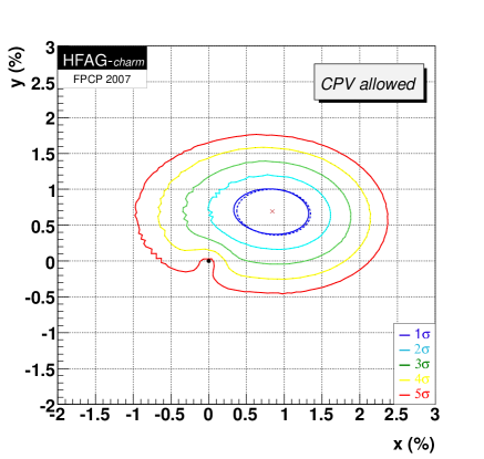
Figure 7: Confidence level contours for $(x,y)$ from combining mixing measurements with CP violation allowed. The dashed blue curve shows the $1\sigma$ contour from the CP conserving case for comparison.

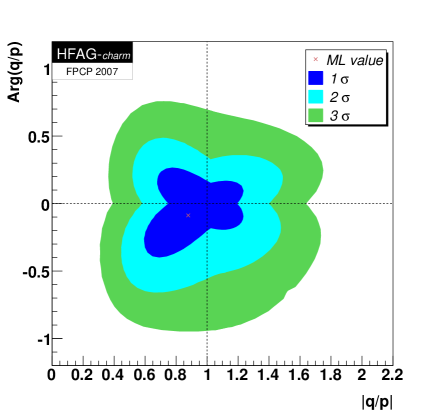
Figure 8: Confidence level contours for $(|q/p|,\phi)$ from combining mixing measurements with CP violation allowed.

V Summary

Evidence of charm mixing has been reported from several experiments in the last year. A new subgroup of HFAG has performed an average of these and other existing charm mixing results. The combined result has a signal significance in excess of 5 standard deviations and gives the mixing parameters

$$x = (8.4^{+3.2}_{-3.4})\times 10^{-3},$$

$$y = (6.9\pm 2.1)\times 10^{-3}.$$

CP violation parameters have also been combined and gives

$$|q/p| = 0.88^{+0.23}_{-0.20},$$

$$\phi = (-0.09^{+0.17}_{-0.19})\mathrm{rad}.$$

This is fully consistent with no CP violation being present in charm mixing. HFAG intends to periodically update these averages as new results become available in order to provide the most precise mixing parameters to the community.

References

- (1) B. Aubert et al. [BABAR Collaboration], Phys. Rev. Lett. 98, 211802 (2007) [arXiv:hep-ex/0703020].
- (2) M. Staric et al. [Belle Collaboration], Phys. Rev. Lett. 98, 211803 (2007) [arXiv:hep-ex/0703036].
- (3) A. J. Schwartz, In the Proceedings of 5th Flavor Physics and CP Violation Conference (FPCP 2007), Bled, Slovenia, 12-16 May 2007, pp 024 [arXiv:0708.4225 [hep-ex]].
- (4) D. M. Asner et al. [CLEO Collaboration], Int. J. Mod. Phys. A 21, 5456 (2006) [arXiv:hep-ex/0607078].
- (5) E. M. Aitala et al. [E791 Collaboration], Phys. Rev. Lett. 83, 32 (1999) [arXiv:hep-ex/9903012].
- (6) J. M. Link et al. [FOCUS Collaboration], Phys. Lett. B 485, 62 (2000) [arXiv:hep-ex/0004034].
- (7) S. E. Csorna et al. [CLEO Collaboration], Phys. Rev. D 65, 092001 (2002) [arXiv:hep-ex/0111024].
- (8) B. Aubert et al. [BABAR Collaboration], Phys. Rev. Lett. 91, 121801 (2003) [arXiv:hep-ex/0306003].
- (9) K. Abe et al. [Belle Collaboration], Phys. Rev. Lett. 88, 162001 (2002) [arXiv:hep-ex/0111026].
- (10) E. M. Aitala et al. [E791 Collaboration], Phys. Rev. Lett. 77, 2384 (1996) [arXiv:hep-ex/9606016].
- (11) C. Cawlfield et al. [CLEO Collaboration], Phys. Rev. D 71, 077101 (2005) [arXiv:hep-ex/0502012].
- (12) U. Bitenc et al. [Belle Collaboration], Phys. Rev. D 72, 071101 (2005) [arXiv:hep-ex/0507020].
- (13) B. Aubert et al. [BABAR Collaboration], Phys. Rev. D 76, 014018 (2007) [arXiv:0705.0704 [hep-ex]].
- (14) B. Aubert et al. [BABAR Collaboration], Phys. Rev. Lett. 97, 221803 (2006) [arXiv:hep-ex/0608006].
- (15) B. Aubert et al. [BABAR Collaboration], arXiv:hep-ex/0607090.
- (16) D. M. Asner et al. [CLEO Collaboration], Phys. Rev. D 72, 012001 (2005) [arXiv:hep-ex/0503045].
- (17) L. M. Zhang et al. [Belle Collaboration], Phys. Rev. Lett. 99, 131803 (2007) [arXiv:0704.1000].
- (18) L. M. Zhang et al. [BELLE Collaboration], Phys. Rev. Lett. 96, 151801 (2006) [arXiv:hep-ex/0601029].