The impact of magnetic field on the thermal evolution of neutron stars

Abstract

The impact of strong magnetic fields $B>10^{13}$G on the thermal evolution of neutron stars is investigated, including crustal heating by magnetic field decay. For this purpose, we perform 2D cooling simulations with anisotropic thermal conductivity considering all relevant neutrino emission processes for realistic neutron stars. The standard cooling models of neutron stars are called into question by showing that the magnetic field has relevant (and in many cases dominant) effects on the thermal evolution. The presence of the magnetic field significantly affects the thermal surface distribution and the cooling history of these objects during both, the early neutrino cooling era and the late photon cooling era. The minimal cooling scenario is thus more complex than generally assumed. A consistent magneto-thermal evolution of magnetized neutron stars is needed to explain the observations.

It has been long hoped that the comparison of theoretical models for the cooling of neutron stars (NSs) with the direct observation of their thermal emission would help to unveil the physical conditions in the interior of these fascinating objects (Page et al., 2004; Yakovlev & Pethick, 2004). Our knowledge of the cooling history of a NS has been improving as we were refining the physical ingredients that play a key role on the thermal evolution of NSs. In the past, the field has become more exciting every time that a new relevant idea was introduced (direct Urca, superfluidity in dense matter, fast processes due to exotic matter, etc.). However, despite the fact that a number of NSs are known to have large magnetic fields, most studies assumed weak magnetic fields. The main reason for this simplification was that the observed distribution of magnetic fields in radio-pulsars peaks in a region where its effect were thought not to be relevant.

The increasing evidence that most of the nearby NSs with reported thermal emission in the x-ray band of the electromagnetic spectrum have anisotropic surface temperature distributions (Zavlin, 2007; Haberl, 2007), the striking appearance of magnetars (Kaspi, 2007), and the discovery of thermal emission from some high field radio-pulsars (Gonzalez et al., 2005), are indicating that most NSs which can be potentially used to contrast theoretical cooling curves have actually large magnetic fields ($B>10^{13}$ G). The conclusion is that a realistic NS cooling model must not avoid the inclusion of high magnetic fields.

The so-called minimal cooling scenario (see e.g. Page et al., 2004; Yakovlev & Pethick, 2004, for recent reviews) defines the cooling model in which the emissivity is given by slow processes in the core, such as modified Urca and nucleon–nucleon Bremsstrahlung, and enhanced by the neutrino emission from the formation and breaking of Cooper-pairs of superfluid neutrons. On the other hand, if fast neutrino processes (i.e. direct URCA) take place, the evolution of a NS changes dramatically, resulting in the enhanced or fast cooling scenario. Nevertheless, direct URCA only operates in the inner core of high mass NSs for some equations of state.

In this letter, we want to revisit the minimal cooling model considering the effects of magnetic field. If a minimal model must include the minimum number of ingredients (but all the necessary ones) to explain the observations, the magnetic field should be taken into account as well.

The effect of the magnetic field on the surface temperature distribution caused by the anisotropic heat transport in the envelope was studied in a pioneering paper by Greenstein & Hartke (1983). The observational consequences of these models were analyzed for the pulsars Vela and Geminga among others (Page, 1995). Potekhin & Yakovlev (2001) calculated the angular distribution of temperatures in magnetized envelopes taking into account the quantizing effect of the magnetic field on the electrons, and the suppression (enhancement) of the electron thermal conductivity in the direction perpendicular (parallel) to magnetic field lines. Nevertheless, the anisotropy generated in the envelope is not strong enough to be consistent with the observed thermal distribution of some isolated NSs, and it should be originated deeper in the NS crust. The understanding of kinetic properties of matter in NS crusts and envelopes has also been recently improved, with special attention received by the role of ions and phonons (Chugunov and Haensel, 2007), which can be relevant at low temperatures and densities. In addition, the effect of impurities on the heat conduction in a non–perfect lattice is also an open problem that must be considered in the near future.

More recently, crustal confined magnetic fields were considered to be responsible for the surface thermal anisotropy observed in some isolated NSs. Temperature distributions in the crust were obtained as stationary solutions of the diffusion equation with axial symmetry (Geppert et al., 2004). The approach assumed an isothermal core and a magnetized envelope as inner and outer boundary condition, respectively. The results showed important deviations from the crust isothermal case for crustal confined magnetic fields with strengths $B>10^{13}$ G and temperature $T<10^{8}$ K. Same conclusions have been obtained considering not only poloidal but also toroidal components of the magnetic field (Pérez-Azorín et al., 2006a; Geppert et al., 2006). These models succeeded in explaining simultaneously the observed x-ray spectrum, the optical excess, the pulsed fraction, and other spectral features of some isolated NS, such as RX J0720.4-3125 (Pérez-Azorín et al., 2006b).

Although former studies about anisotropic temperature distributions on the cooling history of NSs (Shibanov & Yakovlev, 1996; Potekhin & Yakovlev, 2001) provided very useful information, detailed investigations of heat transport in the non spherical case for different magnetic field geometries have not been available until recently. In Aguilera et al. (2007) we have revisited the cooling of NSs combining the insulating effect of strong non radial fields with the additional source of heating due the Ohmic dissipation of the magnetic field in the crustal region. We have shown that, during the neutrino cooling era and the early stages of the photon cooling era, the thermal evolution is coupled to the magnetic field evolution, and both processes (cooling and magnetic field diffusion) proceed on a similar timescale ($\simeq 10^{6}$ yr). The energy released by magnetic field decay (Joule heating) in the crust is an important heat source that modifies or even controls the thermal evolution of a NS. There is indeed observational evidence of this fact. As shown in Pons et al. (2007), there is a strong correlation between the inferred magnetic field and the surface temperature in a wide range of magnetic fields: from magnetars ($B\geq 10^{14}$ G), through radio-quiet isolated NSs ($B\simeq 10^{13}$ G) down to some ordinary pulsars ($B\leq 10^{13}$ G). The main conclusion is that, rather independently from the stellar structure and the matter composition, the correlation can be explained by heating from dissipation of currents in the crust on a timescale of $\simeq 10^{6}$ yrs.

Table 1Properties of neutron stars with reported thermal emission, ordered by decreasing magnetic field strength.

Source	$T^{\infty}$	$t_{sd}$	$B_{d}$	Ref.
	($10^{6}$ K)	($10^{3}$ yr)	(1013 G)
SGR 1806-20	$7.56^{+1.6}_{-0.7}$	0.22	210	1
SGR 0526-66	$6.16^{+0.07}_{-0.07}$	2.0	73	1
1E 1841-045	$5.14^{+0.02}_{-0.02}$	4.5	71	1
SGR 1900+14	$5.06^{+0.93}_{-0.06}$	1.1	64	1
1RXS J170849-400910	$5.30^{+0.98}_{-1.23}$	9.0	47	1
1E 1048.1-5937	$7.24^{+0.13}_{-0.07}$	3.8	42	1
CXOU J010043.1-721134	$4.44^{+0.02}_{-0.02}$	6.8	39	1
XTE J1810-197	$7.92^{+0.22}_{-5.83}$	17	17	1
4U 0142+61	$4.59^{+0.92}_{-0.40}$	70	13	1
PSR J1718-3718	$1.69^{+0.62}_{-0.23}$	34	7.4	2
1E 2259+586	$4.78^{+0.34}_{-0.89}$	230	5.9	1
CXOU J1819-1458	$1.40^{+0.47}_{-0.47}$	117	5.0	3
PSR J1119-6127	$2.40^{+0.30}_{-0.20}$	1.7	4.1	4
RBS1223	$1.00^{+0.0}_{-0.0}$	1461	3.4	5
RX J0720.4$-$3125	$1.05^{+0.06}_{-0.06}$	1905	2.4	5
PSR B2334+61	$0.65^{+0.13}_{-0.34}$	40.9	0.99	6
PSR B0656+14	$1.25^{+0.03}_{-0.03}$	111	0.47	7
PSR B0531+21 (Crab)	$<1.97$	1.24	0.38	8
PSR J0205+6449	$<1.02$	5.37	0.36	9
RX J0822-4300	$1.75^{+0.15}_{-0.15}$	7.96	0.34	10
PSR B0833-45 (Vela)	$0.68^{+0.03}_{-0.03}$	11.3	0.34	11
PSR B1706-44	$0.82^{+0.01}_{-0.34}$	17.5	0.31	12
PSR J0633+1748	$0.50^{+0.01}_{-0.01}$	342	0.16	7
PSR B1055-52	$0.79^{+0.03}_{-0.03}$	535	0.11	7

References. — (1) SGR/AXP Online Catalogue; (2) Kaspi & McLaughlin (2005); (3) Reynolds, S. P. et al (2006), McLaughlin, M. A. et al. (2007); (4) Gonzalez et al. (2005); (5) Haberl (2007); (6) McGowan et al. (2006); (7) De Luca et al. (2005); (8) Weisskopf et al. (2004); (9) Slane et al. (2004); (10)Zavlin et al. (1999), Hui & Becker (2006); (11) Pavlov et al. (2001); (12) McGowan et al. (2004). For the PSRs, $t_{sd}$ and $B_{d}$ from Pulsar Online Catalogue.

In order to investigate if there is observational evidence that supports our models for the crustal field evolution, we have compared theoretical cooling curves including magnetic field decay with a sample of NSs with reported thermal emission. To obtain the cooling curves we have performed two–dimensional simulations by solving the energy balance equation that describes the thermal evolution of a NS

$$C_{v}\frac{\partial T}{\partial t}-\vec{\nabla}\cdot(\hat{\kappa}\cdot\vec{\nabla}T)=-Q_{\nu}+Q_{\rm J}~{},$$ (1)

where $C_{v}$ is the specific heat per unit volume, $Q_{\nu}$ are energy losses by $\nu$-emission, $Q_{\rm J}$ the energy gains by Joule heating, and $\hat{\kappa}$ is the thermal conductivity tensor, in general anisotropic in presence of a magnetic field. In this equation we have omitted relativistic factors for simplicity. A detailed description of the formalism, the code, and results can be found in Aguilera et al. (2007). The geometry of the magnetic field is fixed during the evolution. As a phenomenological description of the field decay, we have assumed the following law

$$B=B_{0}\frac{\exp{(-t/\tau_{\rm Ohm})}}{1+(\tau_{\rm Ohm}/\tau_{\rm Hall})(1-\exp{(-t/\tau_{\rm Ohm})})}~{},$$ (2)

where $B$ is the magnetic field at the pole, $B_{0}$ its initial value, $\tau_{\rm Ohm}$ is the Ohmic characteristic time, and $\tau_{\rm Hall}$ the typical timescale of the fast, initial Hall stage. In the early evolution, when $t\ll\tau_{\rm Ohm}$, we have $B\simeq B_{0}(1+t/\tau_{{\rm Hall}})^{-1}$ while for late stages, when $t\geq\tau_{\rm Ohm}$, $B\simeq B_{0}\exp(-t/\tau_{{\rm Ohm}})$. This simple law reproduces qualitatively the results from more complex simulations (Pons & Geppert, 2007) and facilitates the implementation of field decay in the cooling of NSs for different Ohmic and Hall timescales.

Our sample of objects includes magnetars, isolated radio-quiet NSs, and radio-pulsars, and it covers about three orders of magnitude in magnetic field strength. Before we discuss our results several caveats should be mentioned. For most NSs, $B$ is estimated by assuming that the lose of angular momentum is entirely due to dipolar radiation. If the magnetic field is constant along the evolution, the dipolar component can be estimated by $B_{d}=3.2\times 10^{19}({P\dot{P}})^{1/2}$ G, where $P$ is the spin period in seconds, and $\dot{P}$ is its time derivative. Alternatively, for a few radio-quiet isolated NSs, $B$ is estimated assuming observed x-ray absorption features are proton cyclotron lines. This association is still controversial and, if true, it should be read as an estimate of the surface field, which is usually larger than the external dipolar component. In order to work with a more homogeneous sample, we have included in our study only those objects for which $\dot{P}$ is available. The quoted magnetic fields are always the spin-down estimate for the dipolar component.

Ages are also subject to a large uncertainty. If the birth spin rate far exceeds the present spin rate and $B$ is considered constant, the age can be estimated by the spin-down age ($t_{sd}=P/2\dot{P}$). In the cases that an independent estimate is available (e.g. a kinematic age), the spin-down age does not necessarily coincide with the other estimation. If one considers magnetic field decay, however, $t_{sd}$ seriously overestimates the true age ($t$). Correcting the spin-down age to include the temporal variation of the magnetic field may help to reconcile the observed discrepancy between the spin-down ages and independent measures of the ages of some of the objects we have included in this analysis. This makes the comparison with observations more meaningful. Other sources of error do probably exist but it is not the purpose of this letter to discuss each observation separately.

As for the temperatures, in general there is no clear way to define error-bars. We have adopted the range of values found in the literature, and we also indicate those cases in which the estimate should be interpreted as an upper limit, more than a measure. This is the case of the Crab pulsar, or even of some magnetars, which show large variations in the flux in the soft x-ray band on a timescale of a few years, indicating that the real thermal component may be that measured during quiescence and that the x-ray luminosity during their active periods might be a result of magnetospheric activity. Following the criteria adopted in Page et al. (2004), most reported temperatures are blackbody temperatures, except for low field radio-pulsars in which the blackbody fit results in an unrealistic small radius of the NS. In these four cases, we took the temperature consistent with Hydrogen atmospheres. We include a list of the sources considered in Table 1, with the corresponding references.

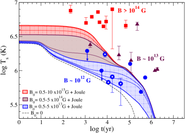
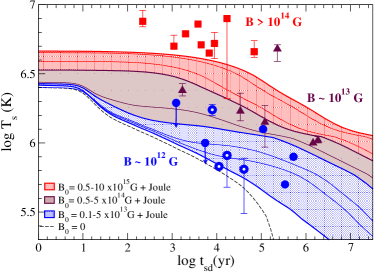
Figure 1.— Cooling curves. Surface temperature at the pole as a function of $t$ (upper panel) and $t_{sd}$ (lower panel) for different $B_{0}$. The magnetar region (red) contains curves for NSs born with $B_{0}>5\times 10^{14}$G. Intermediate field NSs ($5\times 10^{13}$G$\,<B_{0}<5\times 10^{14}$G) evolve within the brown area and the blue region corresponds to NSs with $B_{0}<5\times 10^{13}$G. Observations: squares for sources with $B_{d}>10^{14}$G, triangles with $10^{13}$G$\,<B_{d}<10^{14}$G, and circles with $B_{d}<10^{13}$G. Open circles are temperatures obtained from fits to Hydrogen atmospheres.

In Fig. 1, we show two types of theoretical curves: temperature versus true age (according to the simulation) and temperature versus the spin-down age consistent with the assumptions made on each model about the magnetic field evolution. We have sampled the objects in three groups according to their measured magnetic field: high field NSs with $B_{d}\geq 10^{14}$ G, intermediate field NSs with $10^{13}$ G$<B_{d}<10^{14}$ G and low field NSs for which $B_{d}\leq 10^{13}$ G. We found that this three samples could be explained qualitatively by cooling curves in three different regimes: high, intermediate and low magnetized NSs, in all cases with Joule heating included. Each of these regimes is represented by a set of curves with a given order of magnitude of the initial field, $B_{0}$. We have taken ${\tau_{\rm Ohm}}=10^{6}$ yr and ${\tau_{\rm Hall}}=10^{3}{\rm yr}/B_{0,15}$, where $B_{0,15}$ is $B_{0}$ in units of $10^{15}$ G. The dependence of the results on the decay rates is discussed in Aguilera et al. (2007). These three regions are depicted in Fig. 1 as colored zones. For comparison, the cooling curve corresponding to a non-magnetized NS is represented by a dashed line.

Focusing in the high field (red) region, we see that the effect of the magnetic field is visible from the very beginning of the NS evolution. The initial equilibrium temperature reached in a non–magnetized model may be increased up to a factor of 5 and it is kept nearly constant for a much longer time, up to $10^{4}$ years. The effect of Joule heating is very significant and may help to understand the high temperatures observed in magnetars (Kaspi, 2007), although other physical processes could contribute as well. For instance, the initially higher temperatures result in higher electrical resistivity, therefore accelerating the magnetic field dissipation in an early epoch. We have not yet considered the consistent temperature dependence of the resistivity, in combination with the evolution of the magnetic field geometry. A fully coupled magneto-thermal evolution code should be employed for this purpose (work in progress). The observed temperatures of radio-quiet, isolated NSs could be explained either if they are old NS ($\approx 10^{6}$ years) born as magnetars with $B_{0}=10^{14}$-$10^{15}$ G, or by middle age NSs born with fields in the range of $B_{0}=10^{13}$-$10^{14}$ G, as plotted in the intermediate brown zone of Fig. 1. For intermediate field strengths, the initial effect is not so pronounced but the star can be kept much hotter than non-magnetized NSs during the period from $10^{4}$ to $10^{6}$ yrs. Finally, the effect of the magnetic field in stars born with initial fields of the order of $10^{13}$ G is moderate, but still visible. These would be the case of some radio-pulsars, for which the detection of a thermal component in their spectrum has been reported. For weakly magnetized NSs with $B\simeq 10^{12}$ G, the effect of the magnetic field is small and they can satisfactorily be explained by non-magnetized models, except for very old NSs ($t>10^{6}$ years), as discussed in Miralles et al. (1998).

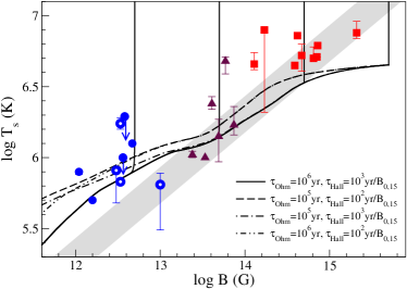
Figure 2.— Surface temperature (at the pole) as a function of the magnetic field. Theoretical curves are shown for different $B_{0}$ and varying $\tau_{\rm Ohm}$ and $\tau_{\rm Hall}$. The grey band corresponds to the HBL (Pons et al., 2007). Observations correspond to Fig. 1.

The fact that the magnetic field plays a relevant role in the thermal evolution of neutron stars at least during the first million years of its life is supported but another observational fact. The magnetic field distribution observed in radio-pulsars is peaked in $3\times 10^{12}$ G. Therefore, assuming no correlation between $B$ and $T$, one would expect to find thermal emission from neutron stars below and above that value in approximately the same number. However, almost all nearby objects for which its temperature is known have fields far exceeding that value. This mismatch between the pulsar field distribution and the thermal emitters field distribution can be easily explained by our assumption: magnetic field decays significantly during the first $10^{6}$ years of a NS life and this effect governs its thermal evolution. As a consequence, NSs with larger fields have higher temperatures and cool slower, increasing the chances to be detected. This hypothesis has been recently outlined by Pons et al. (2007) who reported a strong correlation between the surface temperature and the magnetic field, well approximated by the expression

$$T_{s,6}^{4}\simeq CB_{d,14}^{2}$$ (3)

where $T_{s,6}$ is $T_{s}$ in units of $10^{6}$ K, $B_{d,14}$ is $B_{d}$ in units of $10^{14}$ G, and $C$ is a constant that depends on the thickness of the crust, the Ohmic dissipation timescale, and the ratio between the unknown internal field and the observed external dipole. For typical numbers, $C\simeq 10$. This straight line in a logarithmic plot of temperature versus magnetic field has been named the heat balance line (HBL).

To contrast our results with this hypothesis based on a simple energetics argument, we plot in Fig. 2 the variation of the polar surface temperature $T_{s}$ (usually identified with the hot component of the thermal spectrum) as a function of $B$ for different theoretical curves, and we compare them with the observational data from Table 1. In this $T$-$B$ diagram the thermal history of a NS proceeds as follows. A NS begins its life high on the figure with some initial field $B_{0}$. As it cools it moves vertically downward, until decay of its field provides an energy source able to counterbalance the thermal loses. This causes the trajectory to bend to the left. Then it continues moving down but the temperature and the field evolution are coupled since heating produced by magnetic field depends on the field strength and the cooling mechanisms depend on the temperature. For young magnetars the initial stage is very short because the high field prevents the star to cool down further and the surface temperature remains relatively high. A further evolution proceeds only when the field is also decaying. For low magnetic field stars the drop in the initial temperature is more pronounced and they reach the equilibrium region much later. The region in the diagram where all cooling curves tend to converge is in agreement with the HBL defined in Pons et al. (2007) (indeed it is a band, since not all NSs are necessarily identical). The grey band corresponds to the choice $C=5$-$50$.

Since the initial vertical trajectory is very fast, NSs do not spend much time in that region of the diagram. A clustering of sufficiently old objects in the grey region is expected. Low magnetic field stars reach undetectable low temperatures more quickly, thus they are more difficult to detect than highly magnetized NSs. In the late photon cooling era, since the main mechanism to radiate energy is photons from the star surface, one expects that the correlation given by Eq. (3) is more clear. Although it was a very simplified approximation, we show that our evolution curves approach the HBL slope asymptotically. Finally, it is worth to notice that some objects are crossed by curves belonging to different initial $B_{0}$, so there is no unique determination of the initial conditions.

As a result of this investigation we conclude that consistent magneto-thermal evolution simulations are needed before we can disentangle the properties of the interiors of neutron stars by studying their cooling history. A first step in that direction has been given in this work, showing that the effect of magnetic field decay in the highly resistive crust (as opposed to the highly conductive core) could be very large. It certainly has a significant impact on the thermal evolution of stars with $B\gtrsim 10^{13}$ G. The thermal and magnetic evolution of neutron stars is (at least) a two parameter space, in which the evolutionary tracks of NSs born with different initial conditions (the mass of the object, the initial magnetic field) cannot be properly described by a unique temperature versus age curve. It becomes clear that the minimal model that hopefully will be used to understand neutron stars needs to include the magnetic field structure and evolution.

References

- Aguilera et al. (2007) Aguilera, D. N., Pons, J. A., & Miralles, J. A. 2007, preprint (ArXiv 0710.0854)
- De Luca et al. (2005) De Luca, A., Caraveo, P. A., Mereghetti, S., Negroni, M., & Bignami, G. F. 2005, ApJ, 623, 1051
- Chugunov and Haensel (2007) Chugunov, A. I. and Haensel, P. 2007, MNRAS, 381, 1143
- Geppert et al. (2004) Geppert, U., Küker, M., & Page, D. 2004, A&A, 426, 267
- Geppert et al. (2006) —. 2006, A&A, 457, 937
- Gonzalez et al. (2005) Gonzalez, M. E., Kaspi, V. M., Camilo, F., Gaensler, B. M., & Pivovaroff, M. J. 2005, ApJ, 630, 489
- Greenstein & Hartke (1983) Greenstein, G. & Hartke, G. J. 1983, ApJ, 271, 283
- Haberl (2007) Haberl, F. 2007, Ap&SS, 308, 181
- Hui & Becker (2006) Hui, C. Y. & Becker, W. 2006, A&A, 454, 543
- Kaspi (2007) Kaspi, V. M. 2007, Ap&SS, 308, 1
- Kaspi & McLaughlin (2005) Kaspi, V. M. & McLaughlin, M. A. 2005, ApJ, 618, L41
- McGowan et al. (2004) McGowan, K. E., Zane, S., Cropper, M., Kennea, J. A., Córdova, F. A., Ho, C., Sasseen, T., & Vestrand, W. T. 2004, ApJ, 600, 343
- McGowan et al. (2006) McGowan, K. E., Zane, S., Cropper, M., Vestrand, W. T., & Ho, C. 2006, ApJ, 639, 377
- McLaughlin, M. A. et al. (2007) McLaughlin, M. A. et al. 2007, preprint (ArXiv 0708.1149)
- Miralles et al. (1998) Miralles, J. A., Urpin, V., & Konenkov, D. 1998, ApJ, 503, 368
- Page (1995) Page, D. 1995, ApJ, 442, 273
- Page et al. (2004) Page, D., Lattimer, J. M., Prakash, M., & Steiner, A. W. 2004, ApJS, 155, 623
- Pavlov et al. (2001) Pavlov, G. G., Zavlin, V. E., Sanwal, D., Burwitz, V., & Garmire, G. P. 2001, ApJ, 552, L129
- Pérez-Azorín et al. (2006a) Pérez-Azorín, J. F., Miralles, J. A., & Pons, J. A. 2006a, A&A, 451, 1009
- Pérez-Azorín et al. (2006b) Pérez-Azorín, J. F., Pons, J. A., Miralles, J. A., & Miniutti, G. 2006b, A&A, 459, 175
- Pons & Geppert (2007) Pons, J. A. & Geppert, U. 2007, A&A, 470, 303
- Pons et al. (2007) Pons, J. A., Link, B., Miralles, J. A., & Geppert, U. 2007, Physical Review Letters, 98, 071101
- Potekhin & Yakovlev (2001) Potekhin, A. Y. & Yakovlev, D. G. 2001, A&A, 374, 213
- Reynolds, S. P. et al (2006) Reynolds, S. P. et al. 2006, ApJ, 639, L71
- Shibanov & Yakovlev (1996) Shibanov, Y. A. & Yakovlev, D. G. 1996, A&A, 309, 171
- Slane et al. (2004) Slane, P., Helfand, D. J., van der Swaluw, E., & Murray, S. S. 2004, ApJ, 616, 403
- Weisskopf et al. (2004) Weisskopf, M. C., O’Dell, S. L., Paerels, F., Elsner, R. F., Becker, W., Tennant, A. F., & Swartz, D. A. 2004, ApJ, 601, 1050
- Yakovlev & Pethick (2004) Yakovlev, D. G. & Pethick, C. J. 2004, ARA&A, 42, 169
- Zavlin (2007) Zavlin, V. E. 2007, preprint (ArXiv astro-ph/0702426)
- Zavlin et al. (1999) Zavlin, V. E., Trümper, J., & Pavlov, G. G. 1999, ApJ, 525, 959