Resonant fluxon transmission through impurities

Abstract

Fluxon transmission through several impurities of different strength and type (i.e., microshorts and microresistors), placed in a long Josephson junction is investigated. Threshold pinning current on the impurities is computed as a function of the distance between them, their amplitudes and the dissipation parameter. It is shown that in the case of consequently placed microshorts or microresistors, the threshold pinning current exhibits a clear minimum as a function of the distance between the impurities. In the case of a microresistor, followed by a microshort, an opposite phenomenon is observed, namely the threshold pinning current exhibits maximum as a function of the distance between the impurities.

1 Introduction and the background

The dynamics of magnetic flux propagation in a long Josephson junction (LJJ) is a subject of increasing theoretical and practical interest barone82 ; u98pd . Magnetic flux quantum in a LJJ is a soliton (also known as fluxon) governed by the well-known sine-Gordon (SG) equation. A convenient way to prepare a junction with the required properties is to install various inhomogeneities into it. Up to now substantial work has been devoted to the study of the fluxon motion in the LJJs with point-like impurities. The interaction of a fluxon with a single impurity became a textbook example ms78pra .

On the other hand, the phenomenon of resonant tunneling of an electron through a double-well structure is well-known in quantum mechanics restun . A natural question arises: what is an analog of the quantum-mechanical resonant tunneling in the fluxon dynamics? Resonant soliton transmission has been investigated in detail for non-dissipative systems ksckv92jpa ; zkv94jpsj and complex resonant behaviour has been reported. However, fluxon dynamics in a LJJ cannot be considered without taking into account dissipative effects, which are a consequence of the normal electron tunneling across the insulating barrier. As a result, transmission in a LJJ with constant bias and dissipation can yield only two scenarios: fluxon transmission or fluxon pinning on the impurities. And, consequently, the transmission ratio can attain only two values: zero or unity. Therefore the attention has to be turned toward other characteristic quantities, especially the minimal bias, necessary for the fluxon pinning on impurities.

The present paper aims to investigate fluxon transmission through several (two or more) point-like impurities: microshorts, microresistors or a combination of both. Of particular interest is dependence of the threshold pinning current on the distance between the impurities and their amplitudes.

The paper is organized as follows. In Section 2 we present the model and the basic equations of motion. In the next section we describe the methods of the analysis of the equations and motion and study the fluxon transmission through two microshorts, two microresistors and a microshort and a microresistor as a function of their amplitudes and distance between them. Discussion of the obtained results and final remarks are given in Sec. 4.

2 The model

We consider the long Josephson junction (LJJ) subjected to the external time-independent bias. The main dynamical variable is the difference between the phases $\theta_{2}(x,t)-\theta_{1}(x,t)=\phi(x,t)$ of the macroscopic wave functions of the the superconducting layers of the junction. The time evolution of the phase difference is governed by the perturbed sine-Gordon (SG) equation:

$$\phi_{tt}-\phi_{xx}+\sin\phi=\epsilon f[\phi,\phi_{t};x]~{},$$

$$\epsilon f[\phi,\phi_{t};x]\doteq-\alpha\phi_{t}-\gamma-\sin\phi\sum_{n=1}^{m}\mu_{n}\delta(x-a_{m}).$$ (1)

In this dimensionless equation spacial variable $x$ is normalized to the Josephson penetration depth $\lambda_{J}$, the temporal variable $t$ is normalized to the inverse Josephson plasma frequency $\omega_{J}^{-1}$parameters . Here the bias current $\gamma$ is normalized to the critical Josephson current of the junction and the dimensionless parameter $\alpha$ describes dissipation. It is supposed that there are $N$ impurities in this junction, positioned at the points $x=a_{n}$, $n=1,2,\ldots,N$, $a_{1}\equiv 0<a_{2}<...<a_{m}$, with $\mu_{n}$ being “strength” or amplitude of the $n$th impurity. The impurity is a microshort if $\mu_{n}>0$ and a microresistor if $\mu_{n}<0$.

3 Fluxon transmission

A standard tool for analyzing the fluxon dynamics in Josephson junctions is the McLaughlin-Scott perturbation theory ms78pra . Also, direct numerical integration of the perturbed SG equation (1) will be performed to check the validity of the analytical approximation. We are going to solve the problem for the idealized case of an infinite junction with free ends boundary conditions, however, in actual simulation a sample with length that significantly exceeds the fluxon size will be used.

3.1 Perturbation theory and collective coordinates

Using the perturbation theory, one obtains in the first order the evolution equations for the fluxon parameters, i.e., its center of mass $X$ and fluxon velocity $v$:

$$\dot{v}=\frac{\pi\gamma}{4}(1-v^{2})^{3/2}-\alpha v(1-v^{2})+$$

$$+\frac{1-v^{2}}{2}\sum_{n=1}^{N}\mu_{n}g[X-a(n-1),v]~{},$$ (2)

$$\dot{X}=v-\frac{v}{2}\sum_{n=1}^{N}\mu_{n}[X-a(n-1)]g[X-a(n-1),v],$$ (3)

$$g(X,v)\doteq\frac{\tanh{(X/\sqrt{1-v^{2}})}}{\cosh^{2}{(X/\sqrt{1-v^{2}})}}~{}.$$

For the sake of simplicity in the following only equidistant impurities will be considered, i.e., $a_{n}\equiv a$, $n=1,2,\ldots,N$. Also, only positive values of bias $\gamma$ will be considered. The case of one impurity ($N=1$, $\mu_{1}\equiv\mu$) has been discussed in detail in ms78pra ; kmn88jetp . There exist two characteristic values of the bias current, $\gamma_{c}\equiv 4\sqrt{3}\mu/(9\pi)$ and $\gamma_{thr}$, $\gamma_{c}>\gamma_{thr}$. If $\gamma>\gamma_{c}$, the pinning on the impurity is not possible and only one attractor that corresponds to fluxon propagation does exist. In the interval $\gamma_{thr}<\gamma<\gamma_{c}$ two attractors exist: one corresponds to fluxon pinning on the microshort and another one to fluxon propagation. If $\gamma<\gamma_{thr}$, the only possible regime is fluxon pinning on the impurity. It has been shown ms78pra ; kmn88jetp that there exists a threshold value of the dc bias, which can be approximated as

$$\gamma_{thr}=\frac{\alpha}{\pi}\sqrt{8\mu+\mu^{2}}~{}\left[1-2\alpha\ln 2\right]~{}.$$ (4)

In the case of one microresistor $\mu<0$, the threshold bias has been defined in kmn88jetp as

$$\gamma_{thr}=2\frac{\alpha}{\pi}\left[2\sqrt{\sqrt{2|\mu|}\pi\alpha}+\frac{9}{2}\alpha\ln(\alpha\sqrt{2/|\mu|})\right]~{}.$$ (5)

In the non-relativistic limit ($v\ll 1$) the system (2)-(3) can be rewritten as a Newtonian second order ODE for the particle of mass $8$ (see Refs. ms78pra ; kmn88jetp ):

$$8\ddot{X}+8\alpha\dot{X}=-\frac{\partial U}{\partial X}~{},$$ (6)

$$U(X)=-2\pi\gamma X+U_{0}(X)\equiv-2\pi\gamma X+$$ (7)

$$+2\sum_{n=1}^{m}\frac{\mu_{n}}{\cosh^{2}{[X-a(n-1)]}}~{},~{}~{}\gamma\geq 0~{}.$$

In the case of strongly separated impurities ($a\gg 1$), the potential $U(X)$ has $2N$ extrema [they approximately coincide with the fixed points $X=X_{2k}$, $k=1,2,\ldots,N$, of equations (2)-(3)] where each pair (a minimum and a maximum) is associated with a certain impurity. If there is an impurity at $X=a(k-1)$, the minimum at $X=X_{2k-1}$ always comes before the maximum at $X=X_{2k}$. Microshorts are repelling impurities, thus the fluxon that arrives from $X=-\infty$ decelerates when approaching it and accelerates after passing the impurity until the fluxon velocity reaches the equilibrium value

$$v_{\infty}=\left[1+\left(\frac{4\alpha}{\pi\gamma}\right)\right]^{-1/2}~{}.$$ (8)

Microresitors are attractive impurities, and, as a result, the fluxon accelerates before approaching the microresistor and slows down to the equilibrium velocity (8) after being released from it. Decrease of the distances between the impurities $a$ causes disappearance of some of the extrema via inverse pitchfork bifurcations. The systematic phase plane analysis of equations (2)-(3) for the case of two microshorts has been performed in bp90pla for the SG equation and in pb94pla for the double SG equation. In those papers the behaviour of the fixed points of the system (2)-(3) has been studied as a function of the distance between them, $a$.

Our aim is to determine the threshold current $\gamma_{thr}=\gamma_{thr}(a,\{\mu_{n}\}_{1}^{N};N)$ as a function of the distance between impurities and their amplitudes. In the case of one impurity, $\gamma_{thr}(\mu;1)$ obviously does not depend on the distance $a$. It is described approximately by equations (4) and (5) for the microshort and microresistor, respectively. Some general statement can be made before one proceeds to specific cases. Two important limits should be mentioned. One case corresponds to impurities being separated by the distance much larger the fluxon size. Then the transmission will be governed by the fluxon interaction with each individual impurity. In the opposite limit ($a\rightarrow 0$) the power of all impurities adds up. The effect of the both limits on the threshold current can be written as follows

$$\gamma_{thr}(a,\{\mu_{n}\}_{1}^{N};N)=\left\{\begin{array}[]{c}\gamma_{thr}\left(\sum_{n=1}^{N}\mu_{n};1\right),~{}a\to 0,\\ \max_{1\leq n\leq N}[\gamma_{thr}(\mu_{n};1)],~{}a\to\infty.\end{array}\right.$$ (9)

In the subsections below the transmission through impurities of different polarities (e.g, $\mu_{n}<0$ and $\mu_{n}>0$) will be considered. It appears that for $N\geq 2$ the analytical treatment of equations (2)-(3) is virtually not possible even in the non-relativistic case, especially when none of the limits, described by the equation (9), hold. Therefore equations (2)-(3) are going to be solved numerically.

3.2 Transmission through two microshorts

Consider first the case of two microshorts ($N=2$, $\mu_{1,2}>0$). The problem is tackled in the following way. The fluxon approaches the system of two microshorts from $X=-\infty$ with the equilibrium velocity $v_{\infty}$, given by equation (8). Evolution of the system (2)-(3) on the phase plane $(X,v)$ is shown in Figure 1. Depending on the strength of the bias, three scenarios are possible: trapping on the first microshort (curve 1); trapping on the second microshort, if the external bias is a bit larger (curve 2); or transmission (curve 3).

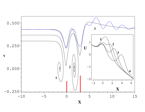
Figure 1: Phase space trajectories of equation (2) for $N=2$ microshorts with $\mu_{1}=0.4$, $\mu_{2}=0.6$ and distance $a=3$ between them. Curve $1$ corresponds to $\gamma=0.04$, curve $2$ - to $\gamma=0.05$ and curve $3$ - to $\gamma=0.06$. Blue curve shows results of direct integration of the equation (1) at $\gamma=0.06$ the using Runge-Kutta method. The fluxon center of mass is defined as $X(t)=\int_{-\infty}^{+\infty}x\phi_{x}dx$ and its velocity as $v(t)=dX(t)/dt$. Dissipation for all cases is $\alpha=0.1$. The inset shows the effective potential $U(X)$ [equation (7)] for $\mu_{1}=0.4,\mu_{2}=0.6$, $\gamma=0.05$, $a=1$ (curve 1), $a=1.7$ (curve 2), $a=2.5$ (curve 3) and $a=4$ (curve 4). Red vertical bars denote locations of the microshorts and the lengths of the bars is proportional to the microshort amplitudes, $\mu_{1,2}$.

If the microshorts are too close to each other, trapping on the second microshort does not happen (see references bp90pla ; pb94pla for details). We note that direct numerical simulations of the perturbed SG equation (1) (curve 4 of Figure 1) are in good correspondence with the trajectories of the system (2). The oscillations after the collision with the microshort can be attributed to the fluxon radiation (not accounted by the first order perturbation theory) and errors in determination of the fluxon center.

The systematic evaluation of the threshold current $\gamma_{thr}$ as a function of the distance $a$ for different values of $\mu_{1}$ and $\mu_{2}$ is shown in Figure 2. The resonant nature of the dependence of $\gamma_{thr}$ on $a$ for $\mu_{1}<\mu_{2}$ can be observed clearly. While in the respective limiting cases it satisfies equation (9), a resonant value $a=a_{r}$ appears, at which the threshold current attains its minimal value.

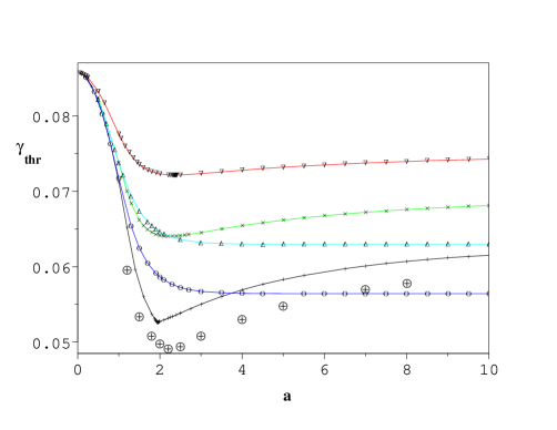
Figure 2: Threshold pinning current as a function of the distance between the microshorts for $\mu_{1}=0.6$, $\mu_{2}=0.4$ ($\Delta$); $\mu_{1}=\mu_{2}=0.5$ ($\circ$); $\mu_{1}=0.4$, $\mu_{2}=0.6$ ($+$); $\mu_{1}=0.3$, $\mu_{2}=0.7$ ($\times$); $\mu_{1}=0.2$, $\mu_{2}=0.8$ ($\nabla$). Results, obtained via direct numerical integration of the equations of motion for $\mu_{1}=0.4$, $\mu_{2}=0.6$ are shown by $\oplus$.

The explanation of the resonant transmission can be done on the following qualitative argument. The analysis of the phase portraits in Figure 1 shows that after being released from the microshort, the fluxon accelerates in order to regain its equilibrium velocity $v_{\infty}$. This acceleration occurs in such a way that for some short interval the fluxon velocity exceeds the equilibrium value $v_{\infty}$. Therefore the fluxon has kinetic energy, which is larger than it was while approaching the microshort from $X=-\infty$, and consequently it has enough energy to pass the microshort with the amplitude larger than $\mu_{1}$. Obviously, the best transmission would take place if $a$ slightly exceeds $|X_{2}-X_{1}|$. The estimation of the resonant distance $a_{r}$ can be made from the analysis of the fluxon dynamics in the non-relativistic limit, given by equations (6)-(7). According to these equations the fluxon can be compared to the particle that slides down along the potential $U(X)=U(X\to\pm\infty)\sim-2\pi\gamma X$. Depending on the value of $\gamma$, it can be trapped in one of the wells of this potential (shown in the inset of Figure 1). If the distance between microshorts is small enough, it can be considered as one microshort with the renormalized strength ${\bar{\mu}}(a)=\mu_{1}+\mu_{2}/\cosh^{2}{a}$. The trapping can occur at the only existing minimum $X_{1}$ (see curve $1$ in the inset of Figure 1) as shown by the trajectory $1$ of Figure 1. As $a$ increases, the potential barriers separate and a local minimum $X_{3}$ appears, as shown by curves $2-4$ in the inset of Figure 1. If a new minimum appears, the trapping can occur also at the second microshort, as shown by the trajectory $2$ of Figure 1. Plots of the potential $U(X)$ clearly demonstrate that the shape of the barrier will be optimal when the minimum at $X=X_{3}$ is quite shallow. Since the half-width of the function $\cosh^{-2}(X)$ is of the order of unity, it is expected that optimal separation of barriers occurs at $a\sim 2$. Numerical evaluation of $a_{r}$ confirms this estimate: $a_{r}=1.94$ (for $\mu_{1}=0.4$, $\mu_{2}=0.6$); $a_{r}=2.24$ ($\mu_{1}=0.3$, $\mu_{2}=0.7$) and $a_{r}=2.36$ (for $\mu_{1}=0.2$, $\mu_{2}=0.8$). If $\mu_{1}\geq\mu_{2}$, the transmission scenario is always determined by the first microshort and the trapping occurs only at $X=X_{1}$. Therefore the dependence $\gamma_{thr}$ on $a$ is monotonically decreasing as shown in Figure 2 for $\mu_{1}=0.6$, $\mu_{2}=0.4$.

It would be of interest to compare how the threshold pinning current depends on the dissipation parameter $\alpha$ and the ratio of the microshort amplitudes $\mu_{1}$ and $\mu_{2}$. Since the resonant distance $a_{r}$ weakly depends on $\mu_{1,2}$ and the pinning current depends strongly on the dissipation constant, it is convenient to normalize $\gamma_{thr}(a,\mu_{1},\mu_{2};2)$ to the pinning current on the strongest microshort
$\max{[\gamma_{thr}(\mu_{1};1),\gamma_{thr}(\mu_{2};1)]}$. In Figure 3 the dependence of the enhancement factor

$$\eta(a,\mu_{1},\mu_{2};2)=\frac{\gamma_{thr}(a,\mu_{1},\mu_{2};2)}{\max{[\gamma_{thr}(\mu_{1};1),\gamma_{thr}(\mu_{2};1)]}}~{},$$ (10)

on the ratio $\mu_{1}/(\mu_{1}+\mu_{2})$ for different values of dissipation is shown. The value of the distance between the microshorts has been fixed to $a=2$. Increase of dissipation does not change much the resonant values of $\mu_{1,2}$. However, the value of the enhancement factor at the minimum decreases significantly.

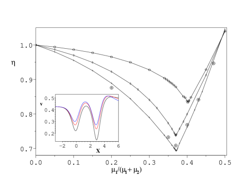
Figure 3: Dependence of the enhancement factor (10) on the ratio $\mu_{1}/(\mu_{1}+\mu_{2})$ $\alpha=0.1$ ($\circ$), $\alpha=0.2$ ($\diamond$) and $\alpha=0.3$ ($+$). Solid lines are used as a guide for an eye. Results, obtained via direct numerical integration of the SG equation with the 4th order Runge-Kutta method for $\alpha=0.3$ are shown by $\oplus$. The inset shows trajectories in the phase plane $(X,v)$ for $\alpha=0.1$, $\gamma=0.06$ (black line); $\alpha=0.2$, $\gamma=0.12$ (red line) and $\alpha=0.3$, $\gamma=0.18$ (blue line). Other parameters are $\mu_{1}=0.4$, $\mu_{2}=0.6$, $a=2$.

In the inset of Figure 3 comparison of the fluxon slowing down on the microshorts is shown for different values of dissipation and dc bias. Note that the ratio $\alpha/\gamma$ was kept constant in order to fix the equilibrium velocity $v_{\infty}$. For stronger dissipation the fluxon slows down to smaller velocities (compare the black and blue curves that correspond to $\alpha=0.1$ and $\alpha=0.3$, respectively). Therefore after release from the microshort the fluxon can accelerate to greater values of velocity. As a result, it has more kinetic energy to pass the second microshort. In other words, for larger dissipation one needs larger bias, $\gamma$. Therefore, the tilt of the potential $U(X)$ increases and it smears out the inhomogeneities, created by the impurities.

It should be emphasized that the validity of the perturbation theory approach has been confirmed by the direct numerical integration of the original perturbed SG equation (1). In Figure 2, $\gamma_{thr}$ has been computed via integration of equation (1) for $\mu_{1}=0.4$ and $\mu_{2}=0.6$. It is evident that the perturbation theory gives qualitatively the same result and the quantitative difference is not very large. Similarly, in Figure 3 the results of the numerical integration of equation (1) with $\alpha=0.3$ are given alongside with the perturbation theory results. A good qualitative and quantitative correspondence between these two types of results is clearly demonstrated. Therefore the usage of the approximation (2)-(3) is justified.

3.3 Transmission through $N>2$ microshorts

Now we extend the results of the previous subsection on the case of more then $N=2$ microshorts. In Figure 4 the dependence of $\gamma_{thr}$ on $a$ for $N=2,3,4,5$ is presented. It clearly demonstrates that addition of an extra impurity to the left from the weakest one decreases further the minimum of the threshold current.

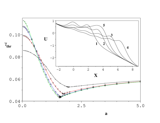
Figure 4: Threshold pinning current as a function of the distance between the microshorts for $\alpha=0.1$, $N=2$, $\mu_{1}=0.4$, $\mu_{2}=0.6$ ($+$); $N=3$, $\mu_{1}=0.27$, $\mu_{2}=0.4$, $\mu_{3}=0.6$ ($\nabla$); $N=4$, $\mu_{1}=0.18$, $\mu_{2}=0.27$, $\mu_{3}=0.4$, $\mu_{4}=0.6$ ($\circ$) and $N=5$, $\mu_{1}=0.12$, $\mu_{2}=0.18$, $\mu_{3}=0.27$, $\mu_{4}=0.4$, $\mu_{5}=0.6$ ($\times$). Solid lines are used as an guide for an eye. The inset depicts the effective potential $U(X)$ [see equation (7)] for the configurations, described in the main figure at $\gamma=0.05$ and for the same values of $\{\mu_{n}\}$: $N=2$, $a=2$ (curve 1); $N=3$, $a=1.7$ (curve 2); $N=4$, $a=1.6$ (curve 3); $N=5$, $a=1.6$ (curve 4) and $a=1$ (curve 5).

The explanation can be easily seen with the help of the effective potential $U(X)$ [see equation (7)]. Its shape changes significantly when extra microshorts are added. Comparing curves 1 and 2 in the inset of Figure 4 one can see that the energy barrier, which the fluxon should cross, lowers. Adding yet another microshort further lowers the barrier (see curves 3 and 4), so that in the interval $0<X<(N-1)a$ the potential barrier almost turns into the decaying slope which is less steep then $-2\pi\gamma X$. Decrease of $a$ leads to the gradual raising of this slope (compare curves 4 and 5) and consequently to increase of $\gamma_{thr}$.

3.4 Transmission through microresistors

A microresistor is an attracting impurity, therefore the fluxon accelerates when approaching it and decelerates back to $v=v_{\infty}$ after passing through or remains trapped if its velocity (and consequently the external bias current) is less than the threshold value. The effective potential $U(X)$ for a microresistor corresponds to the potential well. If two different microresistors are added consequently, the fluxon can be trapped on the first or on the second one, or, if the bias is large enough, pass through. In Figure 5 the phase portraits for the system with $N=2$ microresistors is shown. The change of the shape of $U(X)$ for the different distances between the microresistors is shown in the inset of Figure 5.

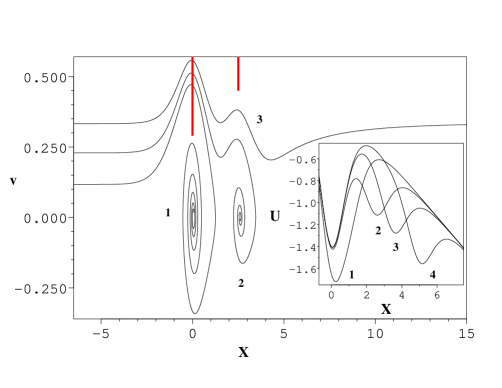
Figure 5: Phase space trajectories of equations (2)-(3) for $N=2$ microresistors with $\mu_{1}=-0.7$, $\mu_{2}=-0.3$ and distance $a=2.5$ between them. Curve $1$ corresponds to $\gamma=0.015$, curve $2$ - to $\gamma=0.03$ and curve $3$ - to $\gamma=0.045$. Dissipation for all cases is $\alpha=0.1$. The inset shows the effective potential $U(X)$ [equation (7)] for $\mu_{1}=-0.7,\mu_{2}=-0.3$, $\gamma=0.03$, $a=1$ (curve 1), $a=2.5$ (curve 2), $a=3.5$ (curve 3) and $a=5$ (curve 4). Red vertical bars denote locations of the microresistors and the lengths of the bars is proportional to their amplitudes, $\mu_{1,2}$.

The computation of the threshold current $\gamma_{thr}$ shows that resonant fluxon transmission is possible if $\mu_{1}<\mu_{2}$ and does not happen if $\mu_{1}\geq\mu_{2}$ (see Figure 6a). Explanation of this phenomenon is similar to the case of two microshorts. If the microresistors are located very close to each other, then their amplitudes add up and the fluxon interacts with the microresistor of the amplitude $\mu\simeq\mu_{1}+\mu_{2}$. When the impurities start to separate, the effective energy barrier which the fluxon should surmount, lowers (compare curve $1$ with curves $2$ and $3$ in the inset Figure 6). The distance between the wells becomes optimal for the best fluxon transmission before they are completely separated (compare curves $3$ and $4$).

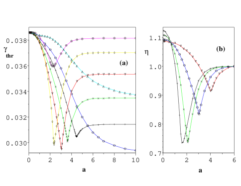
Figure 6: Panel (a). Threshold pinning current as a function of the distance between two microresistors for $\mu_{1}=-0.3$, $\mu_{2}=-0.7$ ($\Delta$); $\mu_{1}=\mu_{2}=-0.5$ ($\circ$); $\mu_{1}=-0.6$, $\mu_{2}=-0.4$ ($+$); $\mu_{1}=-0.7$, $\mu_{2}=-0.3$ ($\times$); $\mu_{1}=-0.8$, $\mu_{2}=-0.2$ ($\nabla$); $\mu_{1}=-0.9$, $\mu_{2}=-0.1$ ($\diamond$) and $\mu_{1}=-0.97$, $\mu_{2}=-0.03$ ($\oplus$). Damping coefficient equals $\alpha=0.1$. Panel (b). Enhancement factor $\eta$ [see equation (10)] as a function of $a$ for $\mu_{1}=-0.8$, $\mu_{2}=-0.2$ and different values of damping $\alpha$: $\alpha=0.3$ ($+$), $\alpha=0.2$ ($\times$), $\alpha=0.1$ ($\circ$) and $\alpha=0.05$ ($\nabla$).

In contrast to the transmission through two microshorts, the resonant value $a=a_{r}$ depends strongly on the amplitudes $\mu_{1,2}$. Indeed, for $\mu_{1}=-0.7$, $\mu_{2}=-0.3$ one obtains $a_{r}\simeq 3.62$ and for $\mu_{1}=-0.9$, $\mu_{2}=-0.1$ the resonant distance equals $a_{r}\simeq 2.35$. Comparing curves $2-4$ in the inset of Figure 5, one can notice that the fluxon needs enough kinetic energy to overcome the second maximum, located at $X=X_{4}$. Obviously, if $X_{2}$ and $X_{4}$ are not enough separated, the fluxon will have no time to accelerate in order to avoid trapping on the second microresistor. Therefore the case of curve $3$ is the most optimal one: the height of the barrier at $X_{2}$ is not too large, as compared to the curve $4$ and the distance between $X_{2}$ and $X_{3}$ is enough to gain velocity, sufficient for the successful passage over the second barrier. These considerations, of course, correspond to the situation, when the impurities are not strongly separated. Otherwise only the interaction with the first one would matter. For the same reason the position of the minimal threshold current, $a_{r}$, (see Figure 6b) increases with decrease of the damping parameter $\alpha$. Depth of the minimum decays with decrease of $\alpha$ similarly to the case of two microshorts because with the stronger bias the fluxon can pass through the impurities much easier.

Putting additional microresistors after $\mu_{2}$, $0>\mu_{N}>\cdots>\mu_{2}>\mu_{1}$ further lowers the critical pinning current similarly to the case of $N>2$ microshorts, described in the previous Subsection.

3.5 Transmission through a microshort and a microresistor

Finally, we consider the case when two impurities of different polarity (a microshort and a microresistor) are placed one after another. If the microresistor is located before the microshort ($\mu_{1}<0,\mu_{2}>0$) resonant enhancement of the threshold pinning current does not happen. In Figure 7 (panel a) the phase portraits for this case are shown. The microresistor is an attracting impurity after which the fluxon slows down. On contrary, the microshort is a repelling impurity and the fluxon slows down when approaching it. Therefore it is obvious that by placing impurities in such a way one increases $\gamma_{thr}$ as compared to the case of each individual impurity. The analysis of the effective potential $U(X)$, shown in Figure 7 (panel c), further confirms above considerations. The height of the effective barrier, which the fluxon should overcome, can be greater than the height of the individual barriers, created by the individual impurities. If the impurities are very close their influences cancel each other and the fluxon interacts with the impurity of the strength $-|\mu_{1}|+\mu_{2}$. The dependence of the threshold pinning current $\gamma_{thr}$ on the distance between the impurities is given in Figure 8 (panel a).

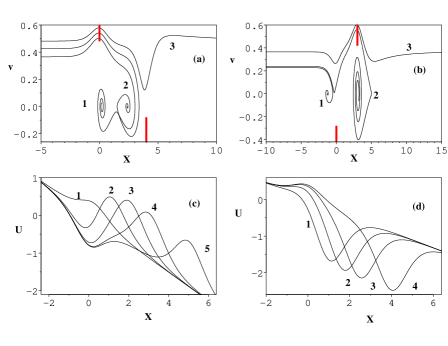
Figure 7: Phase portraits of the fluxon dynamics and effective potentials for the fluxon dynamics in the case of one microshort and one microresistor. Panel (a) shows fluxon trajectories on the phase plane $(X,v)$ for $\alpha=0.1$, $\mu_{1}=-0.4$, $\mu_{2}=0.6$, $a=4$; $\gamma=0.05$ (curve 1), $\gamma=0.06$ (curve 2) and $\gamma=0.07$ (curve 3). Panel (b) shows fluxon trajectories on the phase plane $(X,v)$ for $\alpha=0.1$, $\mu_{1}=0.2$, $\mu_{2}=-0.8$, $a=3$; $\gamma=0.03$ (curve 1), $\gamma=0.0314$ (curve 2) and $\gamma=0.05$ (curve 3). Panel (c) shows the effective potential $U(X)$ for $\mu_{1}=-0.4$, $\mu_{2}=0.6$ and different values of $a$: $a=0.1$ (curve 1), $a=1$ (curve 2), $a=2$ (curve 3), $a=3$ (curve 4) and $a=5$ (curve 5). Panel (d) shows the effective potential $U(X)$ for $\mu_{1}=0.2$, $\mu_{2}=-0.8$ and different values of $a$: $a=1$ (curve 1), $a=1.7$ (curve 2), $a=2.5$ (curve 3) and $a=4$ (curve 4).

For $\mu_{1}=-\mu_{2}=-0.5$ the microshort and microresistor cancel each other for $a=0$, therefore the dependence starts at zero and increases until it reaches the maximal value and then decreases, tending monotonically to the value of $\gamma_{thr}$ that corresponds to one microshort with $\mu=0.5$. The dependence of $\gamma_{thr}$ on $a$ shows an “antiresonant” behaviour because it has a maximum at some certain value of $a$. Analysis of the shape of $U(X)$ from the Figure 7c predicts that the worst transmission would occur when the potential well and the barrier, created by the microresistor and the microshort, respectively, separate from each other far enough to create the highest total barrier (see the curve $3$ of Figure 7c), but not too far (as for the curve $5$ of the same figure) so that each impurity interacts individually with the fluxon.

Consider now the case $\mu_{1}>0,\mu_{2}<0$. The phase portraits for the fluxon dynamics are shown in Figure 7 (panel b). The dependence of the threshold pinning current on the distance between the impurities is shown in Figure 8 (panel b). In the case $\mu_{1}=-\mu_{2}=0.5$ at $a=0$ the impurities cancel each other. When $a$ increases, $\gamma_{thr}$ monotonically increases, tending to the threshold value of one isolated microshort with the amplitude $\mu=0.5$. In this case trapping occurs only on the microshort because analysis of equations (4)-(5) shows that $\gamma_{thr}(0.5;1)>\gamma_{thr}(-0.5;1)$. If $\mu_{1}>|\mu_{2}|$ the dependence of $\gamma_{thr}$ on $a$ is also monotonic. At $a\simeq 0$ the fluxon “feels” both impurities as one microshort with $\mu_{1}-|\mu_{2}|$. When the impurities separate, the contribution of the microresistor to the total amplitude weakens and the threshold current gradually increases till the value $\gamma_{thr}(\mu_{1};1)$.

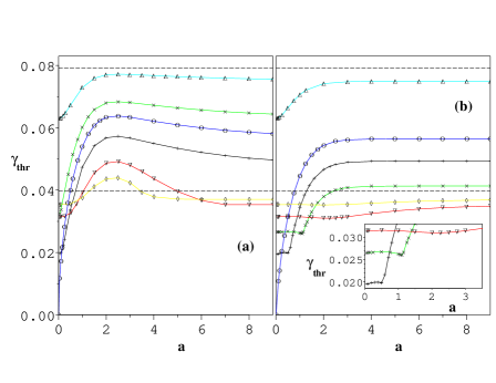
Figure 8: Threshold pinning current as a function of the distance between two impurities $\mu_{1}\mu_{2}<0$ with $\alpha=0.1$. Panel (a): $\mu_{1}=-0.2$, $\mu_{2}=0.8$ ($\Delta$); $\mu_{1}=-0.4$, $\mu_{2}=0.6$ ($\times$); $\mu_{1}=-0.5$, $\mu_{2}=0.5$ ($\circ$); $\mu_{1}=-0.6$, $\mu_{2}=0.4$ ($+$); $\mu_{1}=-0.8$, $\mu_{2}=0.2$ ($\nabla$) and $\mu_{1}=-0.9$, $\mu_{2}=0.1$ ($\diamond$). Panel (b): $\mu_{1}=0.8$, $\mu_{2}=-0.2$ ($\Delta$); $\mu_{1}=0.5$, $\mu_{2}=-0.5$ ($\circ$); $\mu_{1}=0.4$, $\mu_{2}=-0.6$ ($+$); $\mu_{1}=0.3$, $\mu_{2}=-0.7$ ($\times$); $\mu_{1}=0.2$, $\mu_{2}=-0.8$ ($\nabla$) and $\mu_{1}=0.1$, $\mu_{2}=-0.9$ ($\diamond$). Dashed lines correspond to the values $\gamma_{thr}(\pm 1;1)$. Inset shows more detailed picture of $\gamma_{thr}=\gamma_{thr}(a)$.

If $\mu_{1}$ decreases and $|\mu_{2}|$ increases, behaviour of the critical pinning current on $a$ becomes more complicated. Consider first the case $\mu_{1}=0.4$, $\mu_{2}=-0.6$. In the neighbourhood of $a=0$ the system can be considered as a microresistor with the amplitude $\mu_{1}-|\mu_{2}|$. When $a$ increases, the well and the barrier, created by the microshort $\mu_{1}$ start to separate, increasing the depth of the well (created by the microresistor). After some value of the distance $a$ the dependence of $\gamma_{thr}=\gamma_{thr}(a)$ experiences sharp breaking and $\gamma_{thr}$ starts to grow with $a$. The difference between trapping before this breaking point and after it is based on the trapping scenario at $\gamma\leq\gamma_{thr}$. For values of $a$ below the breaking point trapping occurs in the well, created by the microresistor (curve $2$ of Figure 7b) while after the breaking point trapping occurs on the microshort. In other words, the breaking point signals the value of the separation of the impurities, before which the fluxon “feels” them as one microresistor and after which the fluxon “feels” them separately. Decrease of $\mu_{1}$, and subsequent increase of $|\mu_{2}|$ leads to the gradual shift of the breaking point to the right and smoothing of the shape of the dependence $\gamma_{thr}(a)$. Further decrease of $\mu_{1}$ and increase of $|\mu_{2}|$ makes the dependence $\gamma_{thr}(a)$ more and more flat, so that in the limit $\mu_{1}\to 1$, $\mu_{2}\to 0$ it tends to the horizontal line $\gamma_{thr}=\gamma_{thr}(-1;1)$.

4 Conclusions

We have investigated the fluxon transmission in a dc-biased long Josephson junction (LJJ) through two or more impurities of different polarity: microshorts and/or microresistors. We have observed that the threshold pinning current can depend on the distance between impurities in the resonant way for the case of two or more microshorts or two or more microresistors. That means that at some value of the distance the threshold current attains a minimal value, which is less than the threshold current of the strongest impurity. The resonant transmission does not occur if the fluxon interacts with two impurities of different sign: a microshort and a microresistor.

The observed effect should not be confused with the resonant soliton transmission in the non-dissipative cases ksckv92jpa ; zkv94jpsj . In the case of fluxon dynamics in a long Josephson junction the presence of dissipation is unavoidable. Far away from the impurities fluxon exists as an only one attractor of the system with the velocity, predefined by the damping parameter and external bias. Therefore, contrary to the non-dissipative case, there is no sense in computing the transmission ratio, which in our case can take only two values: zero (trapping) and unity (transmission). Also it should not be confused with the fluxon tunneling as a quantum-mechanical object sb-jm97prb across the double-barrier potential, created by two identical microshorts.

The discussed phenomenon can be observed experimentally in an annular LJJ via monitoring the current-voltage (IV) characteristics. For a LJJ with one impurity the fluxon IV curve has a hysteresis-like nature with two critical values of the dc bias (discussed in Section 2). The lower one is the threshold pinning current, which is the smallest current for which fluxon can propagate. Although simulation in this paper have been performed for the infinite junction, there should be no principal differences with the case of an annular junction with sufficiently large length $L\gg\lambda_{J}$. Currently experiments are performed in the junctions $L\sim 10\lambda_{J}$ (see u98pd ) that can be considered as long.

For the future research in this direction it is of interest to find out how the resonant fluxon transmission changes if the actual size of the impurities and the junction width along the $y$-axis are taken into account.

References

- (1) A. Barone, G. Paterno, Physics and Applications of the Josephson Effect, (Wiley, New York, 1982).
- (2) A. V. Ustinov, Physica D 123, 315 (1998).
- (3) D. W. McLaughlin, A. C. Scott. Phys. Rev. A 18, 1652 (1978).
- (4) A. F. J. Levi, Applied Quantum Mechanics, (Cambridge University Press, New York, 2006).
- (5) Yu. S. Kivshar, A. Sanchez, O. Chubykalo, A. M. Kosevich, L. Vazquez, J. Phys. A: Math. Gen. 25, 5711 (1992).
- (6) F. Zhang, Y. S. Kivshar, L. Vazquez, J. Phys. Soc. Jpn. 63, 466 (1994).
- (7) Expressions for the Josephson penetration depth and Josephson plasma frequency and their actual values can be found in barone82 .
- (8) Yu. S. Kivshar, B. A. Malomed, A. A. Nepomnyashchy, Zh. Eksp. Teor. Fiz. 94, 356 (1988) [Sov. Phys. JETP 67, 850 (1988)].
- (9) T. Bountis, St. Pnevmatikos, Phys. Lett. A 143, 221 (1990).
- (10) Th. Pavlopoulos, T. Bountis. Phys. Lett. A 192, 215 (1994).
- (11) A. Shnirman, E. Ben-Jacob, B. Malomed. Phys. Rev. B 56, 14 677 (1997).