arXiv:0712.1120 [hep-ph]

Thermal effects on slow-roll dynamics

Abstract

A description of the transition from the inflationary epoch to radiation domination requires the understanding of quantum fields out of thermal equilibrium, particle creation and thermalisation. This can be studied from first principles by solving a set of truncated real-time Schwinger-Dyson equations, written in terms of the mean field (inflaton) and the field propagators, derived from the two-particle irreducible effective action. We investigate some aspects of this problem by considering the dynamics of a slow-rolling mean field coupled to a second quantum field, using a $\varphi^{2}\chi^{2}$ interaction. We focus on thermal effects. It is found that interactions lead to an earlier end of slow-roll and that the evolution afterwards depends on details of the heatbath.

1 Introduction

Cosmological observations strongly suggest that a stage of accelerated expansion took place in the very early Universe [1, 2]. Such a stage is well described in terms of the dynamics of a scalar field, the inflaton $\phi(t)=\langle\varphi(t,{\mathbf{x}})\rangle$, slow-rolling in a suitable potential $V[\phi]$. Classically, the inflaton equation of motion reads

$$\ddot{\phi}(t)+3H(t)\dot{\phi}(t)+V^{\prime}[\phi(t)]=0,$$ (1.1)

with the Hubble rate determined by the Friedmann equation

$$H^{2}(t)=\frac{\left(\frac{1}{2}\dot{\phi}^{2}(t)+V[\phi(t)]\right)}{3M_{\rm pl}^{2}},$$ (1.2)

where $M_{\rm pl}$ is the Planck mass.

It is natural to assume that the inflaton is coupled directly or indirectly to the Standard Model fields and that after inflation, the energy stored in the inflaton is transfered to excitations of these fields. This can be realised through perturbative reheating [3, 4] or nonperturbative preheating [5, 6, 7, 8, 9, 10, 11, 12, 13] processes. Through scattering, the system eventually reaches thermal equilibrium and a radiation dominated Universe emerges. In quantum field theory, the inflaton evolution in real time is described by a Schwinger-Dyson equation,

$$\ddot{\phi}(t)+3H(t)\dot{\phi}(t)+V^{\prime}[\phi(t)]=-\int_{t_{0}}^{t}dt^{\prime}\,\Sigma_{\phi}(t,t^{\prime})\phi(t^{\prime}),$$ (1.3)

where $t_{0}=0$ is the initial time, taken as the starting point for the evolution. The nonlocal (self-energy like) term $\Sigma_{\phi}(t,t^{\prime})$ contains the interaction with quantum fields and is to be determined, either through some well-motivated ansatz or in terms of a systematic diagrammatic expansion.

Due to the interactions, one may expect a backreaction on the inflaton resulting in, e.g., a modified effective mass parameter and possibly friction. A phenomenological inflaton equation of motion incorporating this would be

$$\ddot{\phi}(t)+\left[3H(t)+\Upsilon(t)\right]\dot{\phi}(t)+V_{\rm eff}^{\prime}[\phi(t)]=0.$$ (1.4)

Various approximations have been invoked to motivate Eq. (1.4) [14, 15, 16, 17, 18]. Effective inflaton dynamics as described by Eq. (1.4) is important for warm inflation [15, 22], in which it is assumed that particles created during inflation interact fast enough such that a quasi-stable nonvacuum state is reached.

For a mean field $\phi(t)$ undergoing small amplitude oscillations in a thermal background, an effective damping rate $\Upsilon$ is indeed generated, and it can be calculated perturbatively in a linear response treatment [23]. However, when the mean field displacement from equilibrium cannot be treated as a small perturbation, as in the case of a slow-rolling inflaton, things are less clear and a fully nonequilibrium treatment is required. This is even more the case if properties of the heatbath depend on the value of the mean field through interactions.

In this paper we will not attempt a full investigation in an expanding background. Instead, we will study some aspects of this problem in a simple inflation-inspired model using the tools of nonequilibrium field theory, i.e. solving the Schwinger-Dyson equation (1.3), as derived from truncations of the two-particle irreducible (2PI) effective action [24, 25]. In section 2 we introduce the model, explain how we deal with the expansion and describe the dynamics of the mean field and fluctuations in absence of most interactions. We write down the Schwinger-Dyson equations to next-to-leading order in a coupling expansion of the 2PI effective action in Section 3. In Section 4 we subsequently solve the lattice discretised integro-differential equations numerically without further approximations. We consider various scenarios and study in particular the role of thermal initial conditions for the two quantum fields in our model. Our findings are summarized in Section 5. In the Appendix we collect several approximations that are well-known in the literature and that are used in the main body of the paper for comparison.

2 Model and free evolution

We consider two interacting scalar fields $\varphi$ and $\chi$ evolving in a flat Friedmann-Robertson-Walker Universe, with the action

$$S=-\int d^{4}x\,\sqrt{-g}\left[\frac{1}{2}g^{\mu\nu}\partial_{\mu}\varphi\partial_{\nu}\varphi+\frac{1}{2}g^{\mu\nu}\partial_{\mu}\chi\partial_{\nu}\chi+\frac{1}{2}m_{\varphi}^{2}\varphi^{2}+\frac{1}{2}m_{\chi}^{2}\chi^{2}+\frac{1}{2}g^{2}\varphi^{2}\chi^{2}\right].$$ (2.1)

The metric is specified by $ds^{2}=dt^{2}-a^{2}(t)d{\mathbf{x}}^{2}$. Hence, the spatial derivatives are given by $\partial_{\bf x}/a(t)$, where ${\bf x}$ is co-moving. The Friedmann equation determines the evolution of the scale factor as

$$\left(\frac{\dot{a}(t)}{a(t)}\right)^{2}\equiv H^{2}(t)=\frac{\langle T^{00}(t)\rangle}{3M^{2}_{\rm pl}},$$ (2.2)

where $\langle T^{00}\rangle$ is the renormalized expectation value of the energy density of matter. We let $\varphi$ play the role of the inflaton: its expectation value $\langle\varphi(t,{\bf x})\rangle=\phi(t)$ is homogeneous and set to some large value initially, $\phi(0)=\phi_{0}$, prompting slow-roll inflation. We take $\langle\chi(t,{\bf x})\rangle=0$ for all times, consistent with the symmetries of the action.

In order to understand the dynamics in this model, we start by considering the classical evolution of $\phi(t)$ without interactions. Its equation of motion is

$$\ddot{\phi}(t)+3H(t)\dot{\phi}(t)+m_{\varphi}^{2}\phi(t)=0,$$ (2.3)

with $H$ given by

$$H^{2}(t)=\frac{\dot{\phi}^{2}(t)+m_{\varphi}^{2}\phi^{2}(t)}{6M_{\rm pl}^{2}}.$$ (2.4)

In the slow-roll limit, $H^{2}(t)=m_{\varphi}^{2}\phi^{2}(t)/6M^{2}_{\rm pl}$, and we find

$$\phi(t)=\phi_{0}-\sqrt{\frac{2}{3}}m_{\varphi}M_{\rm pl}t.$$ (2.5)

Assuming that inflation ends when the slow-roll parameter $\epsilon=\frac{1}{2}M_{\rm pl}^{2}(V^{\prime}[\phi]/V[\phi])^{2}$ equals 1, we find that there is inflation when $\phi/M_{\rm pl}\gtrsim\sqrt{2}$, irrespective of the value of $m_{\varphi}$; a given initial value $\phi_{0}$ corresponds in the slow-roll approximaton to $N_{e}=[(\phi_{0}/M_{\rm pl})^{2}-2]/4$ e-folds before the end of inflation.

The $\chi$ field, coupled to this slow-rolling inflaton, is expanded in terms of creation and annihilation operators as

$$\chi(t,{\bf x})=\int_{\mathbf{k}}\left(a_{\bf k}f_{\bf k}(t)e^{i{{\mathbf{k}}\cdot{\mathbf{x}}}}+a^{\dagger}_{\bf k}f^{*}_{\bf k}(t)e^{-i{{\mathbf{k}}\cdot{\mathbf{x}}}}\right),$$ (2.6)

where

$$\int_{\mathbf{k}}=\int\frac{d^{3}k}{(2\pi)^{3}}.$$ (2.7)

The mode functions $f_{\bf k}(t)$ obey the equation

$$\left[\partial_{t}^{2}+3H(t)\partial_{t}+{\bf k}^{2}/a^{2}(t)+m_{\chi}^{2}+{g^{2}}\phi^{2}(t)\right]f_{\bf k}(t)=0.$$ (2.8)

At this level the inflaton acts as a time-dependent mass.

We now make a practical choice that we will follow throughout this paper: we ignore the expansion of the Universe for the quantum fields (or mode functions) and put $H=0$, $a(t)=1$ in Eq. (2.8), while keeping Hubble friction in the mean field equation. This has the effect of emphasizing the role of scattering and energy transfer during the slow-roll regime and maximises the backreaction of the quantum modes on the mean field by omitting the effect of dilution and redshift. As a result we are not studying inflation, but rather the impact of interactions on a slow-rolling mean field. It allows us to disentangle the direct effect of field theory interactions from the effect of including a $\chi$-component in $T^{00}$. Such a component would influence the inflaton evolution via the Friedmann equation. Neglecting expansion is expected to strongly favour thermalisation. We can make a rough estimate by comparing the expansion rate $H$ to the perturbative damping rate $\Gamma(T)$ [23]. The ratio $\Gamma/H$ is maximal at the end of inflation, and for the largest temperatures used in Section 4 ($T/M_{\rm pl}=4$), we find $\Gamma/H\sim 0.03$. The expansion could therefore have a significant impact on thermalisation. In practice however, the time scales under consideration here are much shorter than the thermalisation time scale, and, as we will see below, equilibration and thermalization will not play a role here.

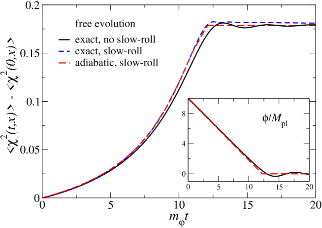
Figure 1: The equal-time correlator $\langle\chi^{2}(t,{\mathbf{x}})\rangle-\langle\chi^{2}(0,{\mathbf{x}})\rangle$ for free evolution of the $\chi$ modes in the mean-field background. Shown are the numerically determined evolution in the exact (full) and the slow-roll (dashed) background, as well as in the adiabatic approximation (long-dashed). The inset shows the mean field during the exact evolution (full) and in the slow-roll approximation (dashed).

In Fig. 1 we show the evolution of the mean field $\phi(t)$ and the (subtracted) equal-time correlator

$$\langle\chi^{2}(t,{\mathbf{x}})\rangle=\int_{\mathbf{k}}\left|f_{\mathbf{k}}(t)\right|^{2},$$ (2.9)

for an initial state in vacuum. The initial value of the mean field is $\phi_{0}/M_{\rm pl}=10>\sqrt{2}$, ensuring an extended slow-roll stage. We show the evolution of $\langle\chi^{2}\rangle$ determined by numerically solving the equations for the mode functions $f_{\mathbf{k}}(t)$ using various approximations detailed in Appendices A.1 and A.2: in the exact mean-field background determined by Eqs. (2.3,2.4), in the slow-roll background (2.5), and in the adiabatic approximation. In the inset the time evolution of the mean field is shown, determined by solving Eqs. (2.3,2.4) numerically and in the slow-roll approximation (2.5). In the latter the evolution is stopped when $\phi(t)$ reaches zero; $\phi(t)$ is kept constant at zero from then on.

During the slow-roll regime the mean field $\phi(t)$ and hence the effective $\chi$ mode energies $\omega_{\mathbf{k}}(t)=[{\mathbf{k}}^{2}+m_{\chi}^{2}+g^{2}\phi^{2}(t)]^{1/2}$ decrease. As a result the equal-time correlator $\langle\chi^{2}\rangle$ increases in time. The sharp increase is described very well in the adiabatic approximation. Therefore it does not correspond to a large amount of particle production. The question we address in the remainder of the paper is whether and how interactions modify this basic scenario.

3 2PI expansion at weak coupling

Corrections to the dynamics considered above arise from quantum and possibly thermal back-reaction effects. These can be deduced from taking the expectation value of the Heisenberg operator equation of motion, yielding

$$\partial_{t}^{2}\langle\varphi(x)\rangle+3H(t)\partial_{t}\langle\varphi(x)\rangle+m_{\varphi}^{2}\langle\varphi(x)\rangle+{g^{2}}\langle\chi^{2}(x)\varphi(x)\rangle=0.$$ (3.1)

The last term can be expanded in terms of connected correlators,

$$\langle\chi^{2}(x)\varphi(x)\rangle=\langle\chi^{2}(x)\rangle\phi(t)+\langle\chi^{2}(x)\varphi(x)\rangle_{\rm connected},$$ (3.2)

using again that $\langle\chi(x)\rangle=0$ and writing $\langle\varphi(x)\rangle=\phi(t)$. As is well-known, keeping only the first term amounts to the Hartree or Gaussian approximation (see Appendix A.3). In that case the effects of interactions reduce to a time-dependent mass. In order to systematically go beyond the Hartree approximation and include effects from the connected three-point correlator in Eq. (3.2), we use a formalism that allows for consistent truncations of the Schwinger-Dyson hierarchy: the two-particle irreducible (2PI) effective action.

The 2PI effective action is a functional written in terms of the mean field $\phi$ and the propagators $G_{\varphi}$, $G_{\chi}$ [24],

$$\Gamma[\phi,G_{\varphi},G_{\chi}]= S[\phi]+\frac{i}{2}\mbox{Tr}\ln\,G_{\varphi,0}^{-1}\,+\frac{i}{2}\mbox{Tr}\,G_{\varphi,0}^{-1}G_{\varphi,0}$$ (3.3)

$$+\frac{i}{2}\mbox{Tr}\ln\,G_{\chi,0}^{-1}\,+\frac{i}{2}\mbox{Tr}\,G_{\chi,0}^{-1}G_{\chi,0}+\Gamma_{2}\left[\phi,G_{\varphi},G_{\chi}\right],$$

where $S[\phi]$ is the tree-level action (2.1) written in terms of the mean field, $G_{\varphi/\chi,0}^{-1}$ are the free inverse propagators,

$$iG_{0,\varphi}^{-1}(x,y)= -\left[\square_{x}+m_{\varphi}^{2}\right]\delta_{\mathcal{C}}(x-y),$$ (3.4)

$$iG_{0,\chi}^{-1}(x,y)= -\left[\square_{x}+m_{\chi}^{2}+{g^{2}}\phi^{2}(x)\right]\delta_{\mathcal{C}}(x-y),$$ (3.5)

and $\Gamma_{2}$ is the sum of all two-particle-irreducible diagrams, depending on full propagators and the mean field $\phi$ via the three-point vertex $g^{2}\phi\varphi\chi^{2}$. We follow the notation of Ref. [26].

The series of diagrams in $\Gamma_{2}$ can be truncated, with each set of diagrams corresponding to an approximation to the full theory. In a weak-coupling expansion we include (see Fig. 2),

$$i\Gamma_{2}[\phi,G_{\varphi},G_{\chi}]=\frac{{g^{2}}}{4}\int_{\cal C}d^{4}x\,G_{\varphi}(x,x)G_{\chi}(x,x)$$ (3.6)

$$-\frac{ig^{4}}{4}\int_{\cal C}d^{4}xd^{4}y\,\phi(x)G_{\varphi}(x,y)G_{\chi}^{2}(x,y)\phi(y)-\frac{ig^{4}}{8}\int_{\cal C}d^{4}xd^{4}y\,G_{\varphi}^{2}(x,y)G_{\chi}^{2}(x,y).$$

Diagram b) is formally $\sim g^{4}\phi^{2}$. We have ignored the three-loop diagram that is $\sim g^{8}\phi^{4}$. All $g^{2}\phi^{2}$ insertions are resummed already at the Hartree level: therefore the truncation we use here formally amounts to assuming that $g^{2}\phi$ is small, but with no constraints on $g^{2}\phi^{2}$. Convergence properties of the 2PI coupling expansion were briefly discussed in Ref. [23], and for the $1/N$ expansion in the $O(N)$ model in Refs. [27, 28].

Figure 2: Diagrams included in the 2PI effective action: a) figure 8 b) pippi c) basketball. Full/dashed lines are $\chi$/$\varphi$ propagators. The crosses denote the inflaton mean field.

The equations of motion result from taking the functional derivatives,

$$\frac{\delta\Gamma\left[\phi,G_{\varphi},G_{\chi}\right]}{\delta\phi(x)}=0,\;\;\;\;\;\;\;\;\frac{\delta\Gamma\left[\phi,G_{\varphi},G_{\chi}\right]}{\delta G_{\chi}(x,y)}=0,\;\;\;\;\;\;\;\;\frac{\delta\Gamma\left[\phi,G_{\varphi},G_{\chi}\right]}{\delta G_{\varphi}(x,y)}=0.$$ (3.7)

After going to momentum space and writing the contour propagators and self energies in terms of the statistical and spectral components,

$$G_{\chi}(t,t^{\prime};{\mathbf{k}})=F_{\chi}(t,t^{\prime};{\mathbf{k}})-\frac{i}{2}\,{\rm sign}_{\cal C}(t,t^{\prime})\rho_{\chi}(t,t^{\prime};{\mathbf{k}}),$$ (3.8)

we find the standard equations [26, 29, 30]

$$\left[\partial_{t}^{2}+{\bf k}^{2}+M^{2}_{\varphi/\chi}(t)\right]\rho_{\varphi/\chi}(t,t^{\prime};{\mathbf{k}})= -\int_{t^{\prime}}^{t}dt^{\prime\prime}\,\Sigma_{\varphi/\chi,\rho}(t,t^{\prime\prime};{\mathbf{k}})\rho_{\varphi/\chi}(t^{\prime\prime},t^{\prime};{\mathbf{k}}),$$

$$\left[\partial^{2}_{t}+{\bf k}^{2}+M^{2}_{\varphi/\chi}(t)\right]F_{\varphi/\chi}(t,t^{\prime};{\mathbf{k}})= -\int_{0}^{t}dt^{\prime\prime}\,\Sigma_{\varphi/\chi,\rho}(t,t^{\prime\prime};{\mathbf{k}})F_{\varphi/\chi}(t^{\prime\prime},t^{\prime};{\mathbf{k}})$$

$$+\int_{0}^{t^{\prime}}dt^{\prime\prime}\,\Sigma_{\varphi/\chi,F}(t,t^{\prime\prime};{\mathbf{k}})\rho_{\varphi/\chi}(t^{\prime\prime},t^{\prime};{\mathbf{k}}),$$

with

$$M_{\varphi}^{2}(t)= m_{\varphi}^{2}+{g^{2}}\int_{\mathbf{k}}F_{\chi}(t,t;{\mathbf{k}}),$$

$$M_{\chi}^{2}(t)= m_{\chi}^{2}+{g^{2}}\left[\phi^{2}(t)+\int_{\mathbf{k}}F_{\varphi}(t,t;{\mathbf{k}})\right].$$ (3.10)

The nonlocal self-energies originate from diagrams b) and c) and are easiest written in real space. They are

$$\Sigma_{\chi/\varphi}(x,y)= \Sigma_{\chi/\varphi}^{(b)}(x,y)+\Sigma_{\chi/\varphi}^{(c)}(x,y),$$ (3.11)

where

$$\Sigma_{\chi/\varphi,\rho}^{(b)}(x,y)= -2g^{4}\phi(x)\left[F_{\chi}(x,y)\rho_{\varphi/\chi}(x,y)+F_{\varphi/\chi}(x,y)\rho_{\chi}(x,y)\right]\phi(y),$$

$$\Sigma_{\chi/\varphi,F}^{(b)}(x,y)= -2g^{4}\phi(x)\left[F_{\chi}(x,y)F_{\varphi/\chi}(x,y)-\rho_{\varphi/\chi}(x,y)\rho_{\chi}(x,y)/4\right]\phi(y),$$

and

$$\Sigma_{\chi/\varphi,\rho}^{(c)}(x,y)= -2g^{4}\left[F^{2}_{\varphi/\chi}(x,y)-\rho^{2}_{\varphi/\chi}(x,y)/4\right]\rho_{\chi/\varphi}(x,y),$$

$$-4g^{4}F_{\varphi/\chi}(x,y)\rho_{\varphi/\chi}(x,y)F_{\chi/\varphi}(x,y)$$

$$\Sigma_{\varphi/\chi,F}^{(c)}(x,y)= -2g^{4}\left[F^{2}_{\chi/\varphi}(x,y)-\rho^{2}_{\chi/\varphi}(x,y)/4\right]F_{\varphi/\chi}(x,y)$$ (3.13)

$$+g^{4}F_{\chi/\varphi}(x,y)\rho_{\chi/\varphi}(x,y)\rho_{\varphi/\chi}(x,y),$$

The mean field equation is given by

$$\left[\partial^{2}_{t}+3H(t)\partial_{t}+M_{\phi}^{2}(t)\right]\phi(t)=-\int_{0}^{t}dt^{\prime}\,\Sigma_{\phi}(t,t^{\prime})\phi(t^{\prime}),$$ (3.14)

with $M_{\phi}^{2}(t)=M_{\varphi}^{2}(t)$, $H(t)$ determined by Eq. (2.4), and

$$\Sigma_{\phi}(t,t^{\prime})=\Sigma_{\varphi,\rho}^{(c)}(t,t^{\prime};{\mathbf{k}}={\mathbf{0}}).$$ (3.15)

4 Numerical analysis

In order to solve the set of coupled integro-differential equations presented in the previous sections, the system is discretized on a space-time lattice with spatial lattice spacing $a_{s}$ and temporal spacing $a_{t}$. The resulting discretized 2PI equations are solved numerically, see Refs. [30, 25, 23] and references therein for details. The initial density matrix is taken to be Gaussian, such that only the one- and two-point functions need to be initialized. For the one-point functions we take $\dot{\phi}(0)=0$ but a large initial $\phi(0)=\phi_{0}=10M_{\rm pl}$. For the two-point functions we use

$$G_{\chi/\varphi}(t,t^{\prime};{\mathbf{k}})\bigg{|}_{t=t^{\prime}=0}= \frac{n_{\bf k}^{\chi/\varphi,0}+1/2}{\omega_{\bf k}^{\chi/\varphi,0}},$$ (4.1)

$$\partial_{t}\partial_{t^{\prime}}G_{\chi/\varphi}(t,t^{\prime};{\mathbf{k}})\bigg{|}_{t=t^{\prime}=0}= \left(n_{\bf k}^{\chi/\varphi,0}+1/2\right)\omega_{\bf k}^{\chi/\varphi,0},$$ (4.2)

$$\partial_{t}G_{\chi/\varphi}(t,t^{\prime};{\mathbf{k}})\bigg{|}_{t=t^{\prime}=0}= 0,$$ (4.3)

where the initial mode energy is

$$\omega_{\bf k}^{\chi/\varphi,0}=\sqrt{{\mathbf{k}}^{2}+M_{\chi/\varphi}^{2}(0)},$$ (4.4)

and the initial particle number is

$$n_{\bf k}^{\chi/\varphi,0}=\left(\exp\left[\omega_{\mathbf{k}}^{\chi/\varphi,0}/T_{\chi/\varphi}\right]-1\right)^{-1}.$$ (4.5)

For the lattice discretized formulation, an ${\cal O}(a_{t})$ improvement term is added to the RHS of Eq.  (4.3),

$$\frac{1}{a_{t}}\left[G_{\chi/\varphi}(a_{t},0;{\mathbf{k}})-G_{\chi/\varphi}(0,0;{\mathbf{k}})\right]=-\frac{a_{t}}{2}\left(n_{\bf k}^{\chi/\varphi,0}+1/2\right)\omega_{\bf k}^{\chi/\varphi,0},$$ (4.6)

which ensures that, in the Hartree approximation, evolution initialized at the Hartree fixed point [31] remains at that fixed point, for finite $a_{t}$. The initial conditions then read

$$G_{\chi/\varphi}(a_{t},a_{t};{\mathbf{k}})= G_{\chi/\varphi}(0,0;{\mathbf{k}})=\frac{n_{\bf k}^{\chi/\varphi,0}+1/2}{\omega_{\bf k}^{\chi/\varphi,0}},$$ (4.7)

$$G_{\chi/\varphi}(a_{t},0;{\mathbf{k}})= G_{\chi/\varphi}(0,0;{\mathbf{k}})\left[1-\frac{1}{2}\left(a_{t}\omega_{\mathbf{k}}^{\chi/\varphi,0}\right)^{2}\right],$$ (4.8)

We introduce separate initial “temperatures” $T_{\chi,\varphi}$ for the $\chi$ and the $\varphi$ modes, so that several scenarios can be explored. The initial masses $M^{2}_{\chi/\varphi}(0)$ are obtained by solving the gap equations (3.10) at $t=0$ with $\phi=\phi_{0}$. These equations are divergent and we use a simple local mass counterterm to take care of this. A much more sophisticated renormalisation scheme exists [32, 33, 34, 35, 36], but this more straightforward approach has been seen to perform well [23]. For the coupling constant we take ${g^{2}}=1$ throughout. The (renormalized) masses at zero temperature are $m_{\chi}/M_{\rm pl}=0.1$ and $m_{\varphi}/M_{\rm pl}=1$. Finally, the spatial and temporal lattice spacings are taken as $a_{s}M_{\rm pl}=1$ and $a_{t}/a_{s}=0.01$. The spatial lattice discretisation is fairly coarse, especially at early times when $\phi(t)$ is still large. The time discretisation is well under control throughout.

We compare a range of approximations described above and in the Appendix:

1. free: the mean field equation is solved without back-reaction, the $\chi$ propagator is solved in this background (Sec. 2).

2. perturbative: solution of the perturbatively expanded mean-field equation, the $\chi$ propagator is reconstructed in the perturbative coupling expansion (Appendix A.4).

3. Hartree: solution of the 2PI equations keeping diagram a) (Appendix A.3).

4. no pippi: solution to the 2PI equations keeping diagrams a) and c).

5. full: solution of the 2PI equations keeping diagrams a), b) and c).

Approximation 4) is used since it mimics the case considered in Ref. [37], where the mean field equation includes the (perturbatively expanded) Hartree term, but with a dressed $\chi$ propagator. Including the basketball diagram c) amounts to dressing the $\chi$ and $\varphi$ propagators with the sunset self-energy; this affects the mean field only via the equal-time $\chi$ propagator. Comparing 4) and 5) also gives the possibility to assess whether a given effect originates from diagram b) or c).

We now explore different scenarios and vary the initial “temperatures” $T_{\chi/\varphi}$. Explicitly, we take vacuum initial conditions ($T_{\chi/\varphi}=0$), partly thermal conditions ($T_{\chi/\varphi}\neq 0$, $T_{\varphi/\chi}=0$), and thermal conditions ($T_{\chi/\varphi}\neq 0$).

4.1 Vacuum initial conditions

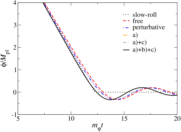
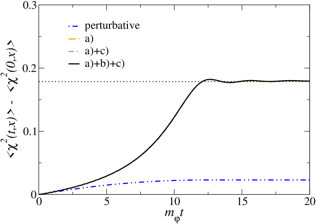
Figure 3: Evolution of the mean field (top) and the equal-time $\langle\chi^{2}\rangle$ correlator (bottom) in the case of vacuum initial conditions, $T_{\chi}=T_{\varphi}=0$. The various approximations are slow-roll, free, perturbative, diagram a) (Hartree approximation), diagrams a) and c) (no pippi), and diagrams a), b) and c) (full) of Fig. 2. The evolution in the latter three cannot be distinguished. In the bottom figure the dotted line indicates the asymptotic result in the adiabatic approximation.

We initialise the system with vacuum propagators in both the $\chi$ and the $\varphi$ sectors, $T_{\chi}=T_{\varphi}=0$. This is the relevant initial condition if we expect inflation to have strongly diluted all matter in the Universe, and all memory of the initial conditions have been lost. In order to heat the Universe, we require reheating (after inflation) or dissipation effects (during inflation) to create particles.

In Fig. 3 (top) the mean field evolution in time is presented, starting in all cases from $\phi_{0}/M_{\rm pl}=10$ with vacuum propagators. Note that the plot only shows the evolution when $\phi(t)/M_{\rm pl}<4$ (or $m_{\varphi}t\gtrsim 7$); for larger values of $\phi$ the slow-roll approximation is very accurate. The evolution in various approximations is shown: slow-roll, free, and perturbative, and the 2PI approximations corresponding to the diagrams of Fig. 2: diagram a) (Hartree approximation), diagrams a) and c) (no pippi), and diagrams a), b) and c) (full). The slow-roll and free result agree initially, but start to deviate somewhat when $m_{\varphi}t\simeq 7$. Slow-roll ends around $\phi\simeq\sqrt{2}M_{\rm pl}$, or $m_{\varphi}t\simeq 10$. When including back-reaction, the three approximations a), a)+c), and a)+b)+c) are practically indistinguishable, but they differ from the free case. This is due to the time-dependent effective mass $M^{2}_{\phi}=m_{\varphi}^{2}+g^{2}\langle\chi^{2}(t,{\mathbf{x}})\rangle$, which increases in time and causes the mean field to roll down faster. The time-dependent part of the mean field mass is shown in Fig. 3 (bottom) in the form of the subtracted equal-time $\langle\chi^{2}\rangle$ correlator, $\langle\chi^{2}(t,{\mathbf{x}})\rangle-\langle\chi^{2}(0,{\mathbf{x}})\rangle$. Here, all approximations behave in the same way, and approach the result predicted by the adiabatic approximation, indicated by the horizontal dotted line. The odd one out is the perturbative approximation, which can only be trusted for times shorter than, say $m_{\varphi}t\simeq 2$. This also explains why the mean field evolution in the perturbative approximation is much closer to the free one; the back-reaction on the mean field is too small.

We find that the evolution is so slow that little departure from adiabaticity is observed and very few particles are created. It is therefore perhaps not surprising that no dissipative effects are seen, and that the Hartree approximation catches all the main features.

4.2 Thermal initial conditions for the $\chi$ field

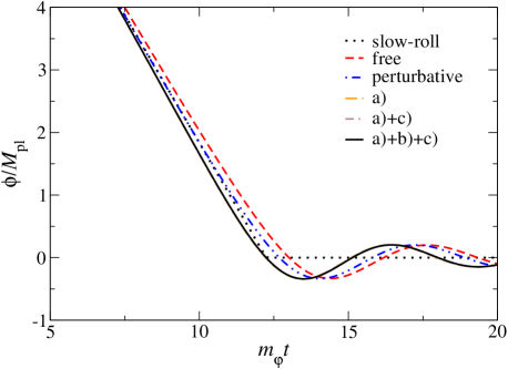
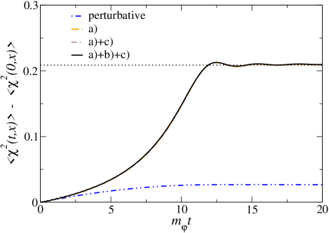
Figure 4: As in Fig. 3, for partly thermal initial conditions, $T_{\chi}/M_{\rm pl}=4$, $T_{\varphi}=0$.

We now consider the scenario where the $\chi$ propagator is initially at finite temperature, $T_{\chi}/M_{\rm pl}=4$, but the $\varphi$ propagator remains in vacuum, $T_{\varphi}=0$. This mimics the case when particle creation has been going on for a while in the $\chi$ propagator, but has not yet trickled down into the $\varphi$ propagator. In this context, the $\varphi$ propagator modes can be thought of as light particle degrees of freedom into which the heavy $\chi$ excitations, with $M_{\chi}\sim g\phi(t)$, may decay. This is motivated by the scenario where additional species are coupled to the $\chi$ sector [38, 39]. If dissipative effects are important, these should show up via the nonlocal diagrams in the propagator and the mean field equation of motion.

In an expanding background, the particles would be redshifted away during inflation, unless sourced by particle creation from the inflaton rolling. By ignoring the expansion in the propagator equation of motion, we keep the initial and any subsequently produced particles, favouring dissipative effects. We note, that as the $\chi$ particles are very heavy initially, the initial particle numbers are very small, $n_{\mathbf{k}}^{\chi}\simeq 1/[\exp{(M_{\chi}/T_{\chi})}-1]\simeq 0.09$.

In Fig. 4 we show the mean field evolution (top) and $\langle\chi^{2}\rangle$ correlator (bottom) for this case. The results are very similar to the ones discussed above, although the back-reaction is stronger due to the $\chi$ heatbath, causing the mean field to roll down slightly faster.

We find therefore that the particles present in the $\chi$ sector influence the evolution of the $\chi$ propagator and the mean field very little.

4.3 Thermal initial conditions for the $\varphi$ field

In the next scenario we initialise the $\varphi$ propagator in thermal equilibrium, with $T_{\varphi}/M_{\rm pl}=4$, and keep the $\chi$ sector in vacuum, $T_{\chi}=0$. This mimics the scenario of Ref. [38], where integrating out the $\varphi$ degrees of freedom is expected to yield a finite width for the $\chi$ particles. In this case particle numbers are of order $n_{\mathbf{k}}^{\varphi}\simeq 1/[\exp{(M_{\varphi}/T_{\varphi})}-1]\simeq 3.5$, so a significant heatbath is present. As long as the $\chi$ mass is larger than the $\varphi$ mass, one may except the heatbath to provide effective damping and a thermal mass. If the coupling is strong enough, the $\chi$ sector may thermalise as well. At the end of inflation, when $M_{\chi}(t)<m_{\varphi}$, the $\varphi$ particles in the heatbath may potentially decay directly into $\chi$ excitations.

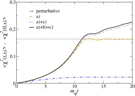
Figure 5: As in Fig. 3, for partly thermal initial conditions, $T_{\chi}=0$, $T_{\varphi}/M_{\rm pl}=4$.

The results for these initial conditions are shown in Fig. 5. The most striking effect is the change to the $\langle\chi^{2}\rangle$ correlator. The presence of the $\varphi$ particles affects the evolution in those approximations that are sensitive to scattering in the heatbath, i.e. the approximations that contain the nonlocal diagrams b) (pippi) and c) (basketball). The Hartree approximation does not incorporate decay or scattering and cannot be applied to this part of the evolution. The fact that both approximations a)+c) and a)+b)+c) show the growing $\langle\chi^{2}\rangle$ correlator indicates that it is mostly due to the presence of the basketball diagram. We note that the effect is largest after slow roll ends, but is visible during the latter part of the slow-roll regime as well. The mean field evolution is very close to the one with vacuum initial conditions, indicating that the $\varphi$ heatbath does not significantly backreact on the mean field evolution using the $\chi$ modes as intermediaries. It should be noted that the perturbative approximation does not know about the $\varphi$ propagator, and so is identical to the case with vacuum initial conditions.

4.4 Thermal initial conditions for both fields

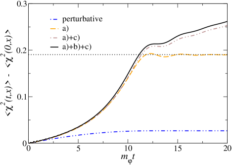
Figure 6: As in Fig. 3, for thermal initial conditions, $T_{\chi}/M_{\rm pl}=T_{\varphi}/M_{\rm pl}=4$.

As the final case, both fields are initialized in thermal equilibrium, with $T_{\chi}/M_{\rm pl}=T_{\varphi}/M_{\rm pl}=4$. This should further enhance the effects of the nonlocal diagrams and mimics the case when interactions are strong enough that the whole system is in equilibrium.

The results are shown in Fig. 6 and are very similar to the case just discussed above. The heatbath of $\varphi$ particles affects the $\chi$ modes mostly after the end of slow roll, where energy transfer from the $\varphi$ to $\chi$ sector is effective. On the other hand, the heatbath of $\chi$ particles makes the effective mean field mass larger than in vacuum, which causes $\phi$ to roll down slightly faster. The nonlocal diagrams b) and c) become essential towards the end of inflation.

For completeness, we note that full equilibration and thermalization takes place on much longer time scales. This has been studied in detail using the loop expansion we used here in Ref. [40, 23, 41]. Again the inclusion of diagrams b) and c) are essential for this.

5 Conclusions

The main goal of this work was to apply techniques of out-of-equilibrium quantum field theory to the problem of interacting quantum fields during and after a slow-roll regime. Although this topic has a long history, a number of assumptions, approximations and ansätze are usually invoked along the way. Here we have employed a systematic formulation based on the loop expansion of the 2PI effective action. We considered a model where the slow-rolling field $\varphi$ is coupled to a second scalar field $\chi$ via a $\varphi^{2}\chi^{2}$ interaction. In order to separate the question of dissipation and particle creation during slow-roll from the dilution in rapidly expanding spacetimes relevant for inflation, we have treated the quantum modes in Minkowski space but preserved the Hubble friction term in the mean field equation of motion. In this setup the mean field rolls slowly at the early stages, after which a smooth transition to the reheating phase is made. It also allowed us to bypass technical issues regarding the numerical solution and renormalisation in expanding space-times.

We have studied several scenarios, corresponding to vacuum and thermal initial conditions in the $\varphi$ and/or $\chi$ sector. The feature dominating the dynamics arises from the interplay between the mean field and the equal-time $\langle\chi^{2}\rangle$ correlator. During the slow-roll regime, the $\langle\chi^{2}\rangle$ correlator increases significantly which results in an increasing effective mean field mass. This effect is not important during the slow-roll stage, but eventually the increasing mean field mass drives the evolution away from slow-roll, such that this regime ends earlier than in the absence of interactions. We found that this is the main source of back-reaction on the mean field. It is already included at the level of the Hartree approximation and is well reproduced by the adiabatic approximation. The presence of the heatbaths affects the later stages of the evolution in various ways. A heatbath of $\chi$ particles mainly speeds up the end of slow roll, since it results in a larger effective mean field mass. A heatbath of $\varphi$ particles is important for the evolution of the $\chi$ modes, due to the possibility of creating $\chi$ particles from $\varphi$ particles. This effect is important mostly at the end of and after slow roll. In this case it is essential to include nonlocal diagrams beyond the mean field/Hartree approximation, which fails to capture this effect. In all scenarios the perturbative approximation was found to not perform very well and to be at best qualitatively valid for very early times, even in the slow-roll regime.

Particle creation and thermal back-reaction effects are crucial in warm inflation. We believe that the scenario would benefit from being recast in the 2PI formalism, since in that case no quasi-particle or equilibrium assumptions would have to be imposed on the propagators. Also, the 2PI expansion systematically includes all the scattering and dissipation effects relied upon in warm inflation. For the parameter values used in this work, we did not reach a warm inflation regime.

2PI resummed equations of motion have been successfully applied to reheating dynamics [42, 13]. There is still the issue of the numerical implementation in expanding backgrounds, addressed in Refs. [43, 44, 45]. Clearly, a complete description of inflationary dynamics requires this to be resolved.

Acknowledgements. We thank Jan Smit, Arjun Berera, Rudnei Ramos and Ian Moss for discussion. G.A. is supported by a PPARC Advanced Fellowship. A.T. is supported by the PPARC SPG “Classical Lattice Field Theory” and by the Academy of Finland Grant 114371. This work was partly conducted on the COSMOS Altix 3700 supercomputer, funded by HEFCE and PPARC in cooperation with SGI/Intel, and on the Swansea Lattice Cluster, funded by PPARC and the Royal Society.

Appendix A Further approximations

In this Appendix, we present a set of approaches for approximating the local correlator $G_{\chi}(x,x)=\langle\chi^{2}(x)\rangle$. These are all well-known in the literature and are used in the main body of the paper for comparison.

A.1 WKB ansatz, adiabaticity and particle creation

We consider the evolution of the mode functions, determined by

$$\ddot{f}_{\bf k}(t)+\omega_{\mathbf{k}}^{2}(t)f_{\bf k}(t)=0,$$ (A.1)

with

$$\omega_{\mathbf{k}}(t)=\left[{\mathbf{k}}^{2}+m_{\chi}^{2}+\delta m^{2}(t)\right]^{\frac{1}{2}},\;\;\;\;\;\;\delta m(t)=g\left(\phi_{0}-\sqrt{\frac{2}{3}}M_{\rm pl}m_{\varphi}t\right).$$ (A.2)

As a first approximation it is instructive to introduce a WKB ansatz of the form [46]

$$f_{\mathbf{k}}(t)=\frac{1}{\sqrt{2\Omega_{\mathbf{k}}(t)}}\exp\left[-i\int_{0}^{t}dt^{\prime}\,\Omega_{\mathbf{k}}(t^{\prime})\right].$$ (A.3)

It is assumed that $\Omega_{\mathbf{k}}(t)>0$ for all $t$. Inserting this into Eq. (A.1) one finds that

$$\Omega_{\mathbf{k}}^{2}=\omega_{\mathbf{k}}^{2}-\frac{1}{2}\frac{\ddot{\Omega}_{\mathbf{k}}}{\Omega_{\mathbf{k}}}+\frac{3}{4}\frac{\dot{\Omega}_{\mathbf{k}}^{2}}{\Omega_{\mathbf{k}}^{2}}.$$ (A.4)

In the adiabatic limit time derivatives are small and $\Omega_{\mathbf{k}}(t)\approx\omega_{\mathbf{k}}(t)$, such that

$$\Omega_{\mathbf{k}}^{2}=\omega_{\mathbf{k}}^{2}-\frac{1}{2}\frac{\ddot{\omega}_{\mathbf{k}}}{\omega_{\mathbf{k}}}+\frac{3}{4}\frac{\dot{\omega}_{\mathbf{k}}^{2}}{\omega_{\mathbf{k}}^{2}}+\ldots$$ (A.5)

Therefore the adiabatic approximation is valid provided

$$\frac{\dot{\omega}_{\mathbf{k}}}{\omega_{\mathbf{k}}^{2}}\ll 1,\;\;\;\;\;\;\;\;\;\;\;\;\frac{\ddot{\omega}_{\mathbf{k}}}{\omega_{\mathbf{k}}^{3}}\ll 1.$$ (A.6)

The (adiabatic) particle number is then given by

$$n_{\mathbf{k}}(t)=\frac{1+2n_{\mathbf{k}}^{0}}{2\omega_{\mathbf{k}}(t)}\left[|\dot{f}_{\mathbf{k}}(t)|^{2}+\omega_{\mathbf{k}}^{2}(t)|f_{\mathbf{k}}(t)|^{2}\right]-\frac{1}{2}\simeq n_{\mathbf{k}}^{0}+{\cal O}\left(\dot{\omega}_{\mathbf{k}}^{2}/\omega_{\mathbf{k}}^{4}\right),$$ (A.7)

where $n_{\mathbf{k}}^{0}$ is the initial $\chi$ particle number present in mode ${\mathbf{k}}$. This is the usual adiabatic result: particle creation is controlled by the rate of change $\dot{\omega}_{\mathbf{k}}/\omega_{\mathbf{k}}^{2}$ [46].

However, the absence (or suppression) of particle creation does not mean that equal-time correlators are constant. For the equal-time correlator

$$\langle\chi(t,{\mathbf{x}})\chi(t,{\mathbf{y}})\rangle=G_{\chi}(t,t;{\mathbf{x}}-{\mathbf{y}})=\int_{\mathbf{k}}e^{i{\mathbf{k}}\cdot({\mathbf{x}}-{\mathbf{y}})}G_{\chi}(t,t;{\mathbf{k}}),$$ (A.8)

we find from the expressions above that

$$G_{\chi}(t,t;{\mathbf{k}})=\left(1+2n_{\mathbf{k}}^{0}\right)|f_{\mathbf{k}}(t)|^{2}\approx\left(1+2n_{\mathbf{k}}^{0}\right)\frac{1}{2\omega_{\mathbf{k}}(t)}.$$ (A.9)

Therefore we find that this equal-time correlator grows in time, with a time dependence directly determined by the time dependence of the mean field, since $\omega_{\mathbf{k}}(t)\sim\phi(t)$ for small $k$. Similarly, the (unrenormalized) energy density in the $\chi$ modes,

$$E_{\chi}(t)=\int_{\mathbf{k}}\frac{\omega_{\mathbf{k}}(t)}{2}\left(2n_{\mathbf{k}}(t)+1\right)\simeq\int_{\mathbf{k}}\frac{\omega_{\mathbf{k}}(t)}{2}\left(2n_{\mathbf{k}}^{0}+1\right),$$ (A.10)

decreases in time as $\phi(t)$ rolls down.

A.2 Exact solution

In certain mean field backgrounds, the mode equation (A.1) can be solved in closed form. In Ref. [39], we considered exponential time dependence $\phi(t)\sim e^{-\gamma t/2}$ (or $\delta m^{2}(t)\sim e^{-\gamma t}$) and found the analytical solution in terms of Bessel functions. We now perform a similar calculation for a slow-rolling mean field in a $\phi^{2}$ potential, where $\phi(t)$ is given by Eq. (2.5).

It is useful to define

$$\kappa\equiv\left(-\frac{d\delta m(t)}{dt}\right)^{\frac{1}{2}}=\left(g\sqrt{\frac{2}{3}}M_{\rm pl}m_{\varphi}\right)^{\frac{1}{2}},$$ (A.11)

and write

$$f_{\mathbf{k}}(t)=\exp\left(ig\phi_{0}t+\frac{i}{2}\kappa^{2}t^{2}\right)h_{\mathbf{k}}(t).$$ (A.12)

We find that $h_{\mathbf{k}}(t)$ satisfies

$$\ddot{h}_{\mathbf{k}}(t)+2i\delta m(t)\dot{h}_{\mathbf{k}}(t)+\left(\omega_{\mathbf{k}}^{2}-i\kappa^{2}\right)h_{\mathbf{k}}(t)=0,$$ (A.13)

where $\omega_{\mathbf{k}}=\sqrt{{\mathbf{k}}^{2}+m_{\chi}^{2}}$ [such that $\omega_{\mathbf{k}}^{2}(t)=\omega_{\mathbf{k}}^{2}+\delta m^{2}(t)$]. Changing variables to

$$x=\frac{\delta m(t)}{\sqrt{i}\kappa},$$ (A.14)

yields Hermite’s equation,

$$h_{\mathbf{k}}^{\prime\prime}(x)-2xh_{\mathbf{k}}^{\prime}(x)+2\nu_{\mathbf{k}}h_{\mathbf{k}}(x)=0,$$ (A.15)

where

$$\nu_{\mathbf{k}}=-\frac{1}{2}\left(1+i\frac{\omega_{\mathbf{k}}^{2}}{\kappa^{2}}\right).$$ (A.16)

The solution reads

$$h_{\mathbf{k}}(x)=A_{\mathbf{k}}H_{\nu_{\mathbf{k}}}(x)+B_{\mathbf{k}}\,{}_{1}F_{1}\left(-\frac{\nu_{\mathbf{k}}}{2},\frac{1}{2},x^{2}\right),$$ (A.17)

where $H_{\nu}(x)$ is a Hermite function and ${}_{1}F_{1}(\alpha,\beta,\gamma)$ is Kummer’s confluent hypergeometric function [47]. The coefficients $A_{\mathbf{k}}$ and $B_{\mathbf{k}}$ are determined by the initial conditions, $f_{\mathbf{k}}(0)=1/\sqrt{2\Omega_{\mathbf{k}}}$ and $\dot{f}_{\mathbf{k}}(0)=-i\Omega_{\mathbf{k}}f_{\mathbf{k}}(0)$, where $\Omega_{\mathbf{k}}=\sqrt{\omega_{\mathbf{k}}^{2}+\delta m^{2}(0)}$. We find that

$$A_{\mathbf{k}}= \frac{1}{\sqrt{2\Omega_{\mathbf{k}}}D_{\mathbf{k}}}\left[\alpha^{(22)}_{\mathbf{k}}+i\Omega_{\mathbf{k}}\alpha^{(12)}_{\mathbf{k}}\right],$$ (A.18)

$$B_{\mathbf{k}}= \frac{-1}{\sqrt{2\Omega_{\mathbf{k}}}D_{\mathbf{k}}}\left[\alpha^{(21)}_{\mathbf{k}}+i\Omega_{\mathbf{k}}\alpha^{(11)}_{\mathbf{k}}\right],$$ (A.19)

where

$$\alpha^{(11)}_{\mathbf{k}}= H_{\nu_{\mathbf{k}}}(x_{0}),$$ (A.20)

$$\alpha^{(12)}_{\mathbf{k}}= {}_{1}F_{1}\left(-\frac{\nu_{\mathbf{k}}}{2},\frac{1}{2},x_{0}^{2}\right),$$ (A.21)

$$\alpha^{(21)}_{\mathbf{k}}= ig\phi_{0}H_{\nu_{\mathbf{k}}}(x_{0})+2\nu_{\mathbf{k}}\sqrt{i}\kappa H_{\nu_{\mathbf{k}}-1}(x_{0}),$$ (A.22)

$$\alpha^{(22)}_{\mathbf{k}}= ig\phi_{0}\,{}_{1}F_{1}\left(-\frac{\nu_{\mathbf{k}}}{2},\frac{1}{2},x_{0}^{2}\right)-2\nu_{\mathbf{k}}\sqrt{i}\kappa x_{0}\,{}_{1}F_{1}\left(1-\frac{\nu_{\mathbf{k}}}{2},\frac{3}{2},x_{0}^{2}\right),$$ (A.23)

with $x_{0}=x(0)=\delta m(0)/\sqrt{i}\kappa$ and $D_{\mathbf{k}}=\alpha^{(11)}_{\mathbf{k}}\alpha^{(22)}_{\mathbf{k}}-\alpha^{(12)}_{\mathbf{k}}\alpha^{(21)}_{\mathbf{k}}$.

A.3 Hartree approximation

In the Hartree approximation, the connected three-point function is neglected and only one- and two-point functions are preserved (Gaussian approximation) [48]. In that case the back-reaction of the $\chi$ modes on the mean field manifests itself as a time-dependent mass and we find

$$\ddot{\phi}(t)+3H(t)\dot{\phi}(t)+M_{\phi}^{2}(t)\phi(t)=0,$$ (A.24)

with

$$M_{\phi}^{2}(t)=m_{\varphi}^{2}+{g^{2}}\langle\chi^{2}(x)\rangle=m_{\varphi}^{2}+{g^{2}}\int_{\mathbf{k}}G_{\chi}(t,t;{\mathbf{k}}).$$ (A.25)

As is well known [48], the Hartree approximation as discussed here is the generalization to time-dependent systems of the standard approach based on the one-loop effective potential in equilibrium. In thermal equilibrium, after integrating out the $\chi$ field, one finds that

$$V_{\rm 1loop}(\phi)=\frac{1}{2}T\sum_{n}\int_{\mathbf{k}}\ln[\omega_{n}^{2}+k^{2}+m_{\chi}^{2}+g^{2}\phi^{2}],$$ (A.26)

where $\omega_{n}=2\pi nT$ ($n\in\mathbb{Z}$) are the Matsubara frequencies. One finds that

$$\frac{\partial V_{\rm 1loop}(\phi)}{\partial\phi}=g^{2}\langle\chi^{2}(x)\rangle\phi,$$ (A.27)

where in equilibrium $\langle\chi^{2}(x)\rangle$ is time-independent and, after performing the Matsubara sum, given by

$$\langle\chi^{2}(x)\rangle=\int_{\mathbf{k}}\frac{1+2n_{B}(\bar{\omega}_{\mathbf{k}})}{2\bar{\omega}_{\mathbf{k}}},\;\;\;\;\;\;\;\;\;\;\;\;\;\;\;\;\bar{\omega}_{\mathbf{k}}=({\mathbf{k}}^{2}+m_{\chi}^{2}+g^{2}\phi^{2})^{\frac{1}{2}}.$$

Here $n_{B}(\omega)=1/(\exp(\omega/T)-1)$ is the Bose distribution.

Out of equilibrium, the evolution of the quantum fluctuations can be determined self-consistently in the Gaussian approximation in terms of the $\varphi$ and $\chi$ propagators as

$$i\left[\partial_{t}^{2}+{\mathbf{k}}^{2}+M_{\varphi}^{2}(t)\right]G_{\varphi}(t,t^{\prime};{\mathbf{k}})= \delta_{\mathcal{C}}(t-t^{\prime}),$$ (A.28)

$$i\left[\partial_{t}^{2}+{\mathbf{k}}^{2}+M_{\chi}^{2}(t)\right]G_{\chi}(t,t^{\prime};{\mathbf{k}})= \delta_{\mathcal{C}}(t-t^{\prime}),$$ (A.29)

with the effective masses

$$M_{\varphi}^{2}(t)= m_{\varphi}^{2}+{g^{2}}\int_{\mathbf{k}}G_{\chi}(t,t;{\mathbf{k}}),$$ (A.30)

$$M_{\chi}^{2}(t)= m_{\chi}^{2}+{g^{2}}\left[\phi^{2}(t)+\int_{\mathbf{k}}G_{\varphi}(t,t;{\mathbf{k}})\right].$$ (A.31)

The Hartree approximation is self-consistent and easily solvable numerically.

A.4 Perturbative approximation

Figure 7: Graphical representation of the dynamics of the $\chi$ propagator (thick line) in the Hartree approximation. The thin line is the lowest order $\chi$ propagator, the thick dashed line the $\varphi$ propagator, and the crosses the mean field background. The second line shows the perturbative expansion discussed in Section A.4.

We can also attempt to include the effect of the time-dependent mean field on the evolution of $G_{\chi}$ in a perturbative manner. This approach is indicated in Fig. 7: while in the Hartree approximation all $\phi^{2}$ insertions are summed nonperturbatively, in the perturbative setup only a single $\phi^{2}$ insertion is preserved. To obtain this, we write

$$G_{\chi}(x,y)\equiv\langle T_{\cal C}\chi(x)\chi(y)\rangle=G_{\chi}^{(0)}(x,y)+{g^{2}}G_{\chi}^{(1)}(x,y)+\mathcal{O}(g^{4}),$$ (A.32)

and solve Eq. (A.29) formally order by order in ${g^{2}}$. In order to avoid large corrections due to the initial large expectation value of the mean field, we write

$$\phi^{2}(x)=\phi^{2}(0)+\left[\phi^{2}(x)-\phi^{2}(0)\right]\equiv\phi_{0}^{2}+\Delta\phi^{2}(x),$$ (A.33)

and treat $g^{2}\Delta\phi^{2}(x)$ as the perturbation. The expansion is therefore expected to be valid for early times only. We also ignore fluctuations of $\varphi$, since $G_{\varphi}(x,x)\ll\phi_{0}^{2}$ after renormalization. In terms of the free inverse propagator,

$$G_{0}^{-1}(x,y)=i\left[\square_{x}+m_{\chi}^{2}+{g^{2}}\phi_{0}^{2}\right]\delta_{\cal C}(x-y),$$ (A.34)

we find the series of equations

$$\int_{\cal C}d^{4}z\,G_{0}^{-1}(x,z)G_{\chi}^{(0)}(z,y)= \delta_{\mathcal{C}}(x-y),$$ (A.35)

$$\int_{\cal C}d^{4}z\,G_{0}^{-1}(x,z)G_{\chi}^{(1)}(z,y)= -i\Delta\phi^{2}(x)G_{\chi}^{(0)}(x,y),$$ (A.36)

etc. The formal solution of the second equation can be written as (see Fig. 7)

$$G_{\chi}^{(1)}(x,y)=-i\int_{\cal C}d^{4}z\,G_{\chi}^{(0)}(x,z)\Delta\phi^{2}(z)G_{\chi}^{(0)}(z,y).$$ (A.37)

To first order in this expansion the mean field equation of motion then reads [37]

$$\left[\partial_{t}^{2}+3H(t)\partial_{t}+\bar{M}_{\varphi}^{2}(t)\right]\phi(t)=ig^{4}\int_{\cal C}d^{4}z\,G_{\chi}^{(0)}(x,z)\Delta\phi^{2}(z)G_{\chi}^{(0)}(z,x)\phi(x),$$ (A.38)

with

$$\bar{M}_{\varphi}^{2}(t)=m_{\varphi}^{2}+{g^{2}}G_{\chi}^{(0)}(x,x).$$ (A.39)

To make the time dependence explicit, we write the propagator along the Schwinger-Keldysh contour in terms of the statistical and spectral components (3.8) and find

$$\left[\partial_{t}^{2}+3H(t)\partial_{t}+\bar{M}_{\phi}^{2}(t)\right]\phi(t)=\int_{0}^{t}dt^{\prime}\,K(t,t^{\prime})\Delta\phi^{2}(t^{\prime})\phi(t),$$ (A.40)

with the kernel

$$K(t,t^{\prime})=2g^{4}\int d^{3}x\,F_{\chi}^{(0)}(t,t^{\prime};{\mathbf{x}})\rho_{\chi}^{(0)}(t,t^{\prime};{\mathbf{x}}).$$ (A.41)

In order to solve Eq. (A.40) numerically, we need to choose a propagator for the memory kernel (A.41). We take the simplest perturbative ansatz

$$F_{\chi}^{(0)}(t,t^{\prime};{\mathbf{k}})= \frac{n_{\mathbf{k}}^{0}+1/2}{\tilde{\omega}_{\mathbf{k}}}\cos[\tilde{\omega}_{\mathbf{k}}(t-t^{\prime})],$$ (A.42)

$$\rho_{\chi}^{(0)}(t,t^{\prime};{\mathbf{k}})= \frac{\sin[\tilde{\omega}_{\mathbf{k}}(t-t^{\prime})]}{\tilde{\omega}_{\mathbf{k}}},$$ (A.43)

depending on the initial energies $\tilde{\omega}_{\bf k}=({\mathbf{k}}^{2}+m_{\chi}^{2}+{g^{2}}\phi_{0}^{2})^{\frac{1}{2}}$. One may think of more elaborate ansätze for these propagators and include e.g. more thermal effects as well as the effect of scattering and decay processes [16, 37]. However, we prefer to discuss this in a systematic approach and employ the 2PI effective action to consider extensions beyond the mean field approximation.

Finally, one can consider further approximations to these equations, using a derivative expansion [49, 50, 37]. However, we will not do so here.

References

• [1] D. N. Spergel et al. [WMAP Collaboration], Astrophys. J. Suppl.  170 (2007) 377 [astro-ph/0603449].
• [2] H. V. Peiris et al. [WMAP Collaboration], Astrophys. J. Suppl.  148, 213 (2003) [astro-ph/0302225].
• [3] A. D. Dolgov and D. P. Kirilova, Sov. J. Nucl. Phys.  51, 172 (1990) [Yad. Fiz.  51, 273 (1990)].
• [4] E. W. Kolb and M. S. Turner, “The Early Universe,” Front. Phys.  69, 1 (1990).
• [5] J. H. Traschen and R. H. Brandenberger, Phys. Rev.  D 42 (1990) 2491.
• [6] L. Kofman, A. D. Linde and A. A. Starobinsky, Phys. Rev. D 56 (1997) 3258 [hep-ph/9704452].
• [7] S. Y. Khlebnikov and I. I. Tkachev, Phys. Rev. Lett.  77, 219 (1996) [hep-ph/9603378].
• [8] T. Prokopec and T. G. Roos, Phys. Rev. D 55 (1997) 3768 [hep-ph/9610400].
• [9] D. Boyanovsky, M. D’Attanasio, H. J. de Vega, R. Holman and D. S. Lee, Phys. Rev.  D 52 (1995) 6805 [hep-ph/9507414].
• [10] D. Boyanovsky, H. J. de Vega, R. Holman and J. F. J. Salgado, Phys. Rev.  D 54 (1996) 7570 [hep-ph/9608205].
• [11] G. N. Felder, J. Garcia-Bellido, P. B. Greene, L. Kofman, A. D. Linde and I. Tkachev, Phys. Rev. Lett.  87 (2001) 011601 [hep-ph/0012142].
• [12] J. Garcia-Bellido, M. Garcia Perez and A. Gonzalez-Arroyo, Phys. Rev.  D 67 (2003) 103501 [hep-ph/0208228].
• [13] A. Arrizabalaga, J. Smit and A. Tranberg, JHEP 0410, 017 (2004) [hep-ph/0409177].
• [14] A. Hosoya and M. A. Sakagami, Phys. Rev.  D 29, 2228 (1984).
• [15] I. G. Moss, Phys. Lett. B 154 (1985) 120.
• [16] M. Morikawa, Phys. Rev.  D 33, 3607 (1986).
• [17] A. Berera and R. O. Ramos, Phys. Rev.  D 63, 103509 (2001) [hep-ph/0101049].
• [18] A. Berera, I. G. Moss and R. O. Ramos, Phys. Rev.  D 76, 083520 (2007) [0706.2793 [hep-ph]].
• [19] D. Boyanovsky, H. J. de Vega, R. Holman, D. S. Lee and A. Singh, Phys. Rev.  D 51 (1995) 4419 [hep-ph/9408214].
• [20] I. D. Lawrie, Phys. Rev.  D 66, 041702 (2002) [hep-ph/0204184].
• [21] I. D. Lawrie, Phys. Rev.  D 67, 045006 (2003) [hep-ph/0209345].
• [22] A. Berera, Phys. Rev. Lett.  75 (1995) 3218 [astro-ph/9509049].
• [23] A. Arrizabalaga, J. Smit and A. Tranberg, Phys. Rev. D 72 (2005) 025014 [hep-ph/0503287].
• [24] J. M. Cornwall, R. Jackiw and E. Tomboulis, Phys. Rev. D 10 (1974) 2428.
• [25] For a recent review, see J. Berges, AIP Conf. Proc.  739 (2005) 3 [hep-ph/0409233].
• [26] G. Aarts, D. Ahrensmeier, R. Baier, J. Berges and J. Serreau, Phys. Rev. D 66 (2002) 045008 [hep-ph/0201308].
• [27] G. Aarts and J. Berges, Phys. Rev. Lett.  88 (2002) 041603 [hep-ph/0107129].
• [28] G. Aarts and A. Tranberg, Phys. Rev.  D 74, 025004 (2006) [hep-th/0604156].
• [29] G. Aarts and J. Berges, Phys. Rev. D 64 (2001) 105010 [hep-ph/0103049].
• [30] J. Berges, Nucl. Phys. A 699 (2002) 847 [hep-ph/0105311].
• [31] G. Aarts, G. F. Bonini and C. Wetterich, Phys. Rev. D 63 (2001) 025012 [hep-ph/0007357].
• [32] H. van Hees and J. Knoll, Phys. Rev.  D 65 (2002) 025010 [hep-ph/0107200].
• [33] H. Van Hees and J. Knoll, Phys. Rev.  D 65 (2002) 105005 [hep-ph/0111193].
• [34] J. P. Blaizot, E. Iancu and U. Reinosa, Nucl. Phys.  A 736 (2004) 149 [hep-ph/0312085].
• [35] J. Berges, S. Borsanyi, U. Reinosa and J. Serreau, Annals Phys.  320 (2005) 344 [hep-ph/0503240].
• [36] A. Arrizabalaga and U. Reinosa, Nucl. Phys.  A 785 (2007) 234 [hep-ph/0609053].
• [37] A. Berera and R. O. Ramos, Phys. Rev. D 71 (2005) 023513 [hep-ph/0406339].
• [38] A. Berera and R. O. Ramos, Phys. Lett. B 567 (2003) 294 [hep-ph/0210301].
• [39] G. Aarts and A. Tranberg, Phys. Lett.  B 650 (2007) 65 [hep-ph/0701205].
• [40] J. Berges and J. Cox, Phys. Lett.  B 517, 369 (2001) [hep-ph/0006160].
• [41] M. Lindner and M. M. Muller, Phys. Rev.  D 73 (2006) 125002 [hep-ph/0512147].
• [42] J. Berges and J. Serreau, Phys. Rev. Lett.  91 (2003) 111601 [hep-ph/0208070].
• [43] D. Boyanovsky, H. J. de Vega and R. Holman, Phys. Rev.  D 49 (1994) 2769 [hep-ph/9310319].
• [44] G. J. Stephens, E. A. Calzetta, B. L. Hu and S. A. Ramsey, Phys. Rev.  D 59 (1999) 045009 [gr-qc/9808059].
• [45] A. Rajantie and A. Tranberg, JHEP 0611, 020 (2006) [hep-ph/0607292].
• [46] Y. Kluger, E. Mottola and J. M. Eisenberg, Phys. Rev.  D 58 (1998) 125015 [hep-ph/9803372].
• [47] M. Abramowitz and I. A. Stegun, Handbook of Mathematical Functions, Dover Publications.
• [48] F. Cooper, S. Habib, Y. Kluger and E. Mottola, Phys. Rev.  D 55 (1997) 6471 [hep-ph/9610345].
• [49] M. Gleiser and R. O. Ramos, Phys. Rev.  D 50 (1994) 2441 [hep-ph/9311278].
• [50] A. Berera, M. Gleiser and R. O. Ramos, Phys. Rev.  D 58 (1998) 123508 [hep-ph/9803394].