Evolving localizations in reaction-diffusion cellular automata

Abstract

We consider hexagonal cellular automata with immediate cell neighbourhood and three cell-states. Every cell calculates its next state depending on the integral representation of states in its neighbourhood, i.e. how many neighbours are in each one state. We employ evolutionary algorithms to breed local transition functions that support mobile localizations (gliders), and characterize sets of the functions selected in terms of quasi-chemical systems. Analysis of the set of functions evolved allows to speculate that mobile localizations are likely to emerge in the quasi-chemical systems with limited diffusion of one reagent, a small number of molecules is required for amplification of travelling localizations, and reactions leading to stationary localizations involve relatively equal amount of quasi-chemical species. Techniques developed can be applied in cascading signals in nature-inspired spatially extended computing devices, and phenomenological studies and classification of non-linear discrete systems.

1 Introduction

Localisations — compact and long-living local disturbances of a medium’s characteristics — are becoming hot topic of interdisciplinary non-linear sciences [19, 18, 8]. They can be found in almost any type of spatially extended non-linear systems, from liquid crystals to monomolecular arrays to reaction-diffusion chemical media [1]. From a computer science point of view, localizations are ideal candidates for elementary processing units in ’free-space’, or collision-based [2] computing devices. The collision-based computation is rooted in logical universality of Conway’s Game of Life [7], Fredkin-Toffoli’s conservative logic [10] and Margolus’s physics of computation [12]. In collision-based computing, quanta of information are represented by compact patterns traveling in an ‘empty’ space and performing computation by mutual collisions. The absence or presence, and type, of traveling patterns encode values of logical variables. The trajectories of patterns approaching a collision site represent input variables. Trajectories of the patterns ejected from a collision represent the results of logical operations, i.e. output variables.

Amongst many possible natural systems supporting localizations, reaction-diffusion chemical media seem to be most appropriate candidates for experimental implementation of collision-based computing architectures. The medium does not require expensive or over-sophisticated equipment, can be handled and tuned with relative ease, and allows for visual identification of experimental results. For example, there is a particular type of reaction-diffusion chemical system, the Belousov-Zhabotinsky reaction in sub-excitable mode [17], that supports the existence of localized wave-fragments (somewhat analogous to dissipative solitons [11]) which can play the role of the ‘billiard-balls’ [12] in a collision-based computing system [3, 9].

In our previous works we have designed and studied a range of hexagonal cellular-automaton models of reaction-diffusion excitable chemical systems, particularly those with concentration dependent inhibition of the activator [4, 21, 5]. We have analyzed three-state totalistic cellular automata on a two-dimensional lattice with hexagonal tiling, and discovered a set of specific rules that support a variety of mobile (gliders) and stationary (eaters) localizations, and generators of localizations (glider guns). In [5] we demonstrated that rich spatio-temporal dynamics of interacting localizations and generators of localizations can be used in implementing purposeful computation, including signal routing, multiple-valued logical operations and finite state machines. Despite success of preliminary studies, and some techniques developed [20] to pinpoint ‘best’ rules supporting localizations, we remained somewhat puzzled and uncertain on whether rules manually selected are good representatives of a set of localization-supporting cell-state transition rules. We therefore applied the full power of evolutionary computation methods to evolve and select all possible rules that support mobile localizations in two-dimensional hexagonal ternary state cellular automata. Results of these studies are discussed in present paper.

The paper is structured as follows. In Sect. 2 we introduce and define ternary state hexagonal cellular automaton. The evolutionary algorithm used to breed glider-supporting rules is outlined in Sect. 3. The evolved set of glider-supporting rules is characterised in Sect. 4. In Sect. 5 we present a set of quasi-chemical reactions derived from the evolved rules. We demonstrate, in Sect. 6, that by integrating the most common glider-supporting rules in one set, we select the rules supporting only stationary localizations. Outcomes of the present studies are discussed in Sect. 7.

2 Reaction-diffusion hexagonal cellular automaton

We study a totalistic cellular automaton, where a cell updates its state depending on just the numbers, not positions, of different cell-states in its neighborhoods. We consider a ternary state automaton. One cell-state, $S$, is a dedicated substrate state: a cell in state $S$, whose neighbourhood is filled only with states $S$, does not change its state ($S$ is a an analogue of quiescent state in cellular automaton models). Two other states, $A$ and $B$, are assigned to be reactants.

The cell-state transition rule can be written as follows:

$$x^{t+1}=f(\sigma_{A}(x)^{t},\sigma_{B}(x)^{t},\sigma_{S}(x)^{t}),$$

where $\sigma_{p}(x)^{t}$ is the number of cell $x$’s neighbors with cell-state $p\in\{A,B,S\}$ at time step $t$. As for all classical cellular automata, all cells updates their states synchronously in discrete time-steps. Our automata are based on a two-dimensional lattice with hexagonal tiling. The neighborhood size is seven: the central cell and its six closest neighbors.

To give a compact representation of the cell-state transition rule, we adopt the formalism in [4], and represent the cell-state transition rule as a matrix ${\bf M}=(M_{ij})$, where $0\leq i\leq j\leq 7$, $0\leq i+j\leq 7$, and $M_{ij}\in\{A,B,S\}$. The output state of each neighborhood is given by the row-index $i$ (the number of neighbors in cell-state $A$) and column-index $j$ (the number of neighbors in cell-state $B$). We do not have to count the number of neighbors in cell-state $S$, because it is given by $7-(i+j)$. A cell with a neighborhood represented by indexes $i$ and $j$ will update to cell-state $M_{ij}$ which can be read off the matrix. In terms of the cell-state transition function this can be presented as follows: $x^{t+1}=M_{\sigma_{A}(x)^{t}\sigma_{B}(x)^{t}}$.

How do matrix ${\bf M}$ entries correspond to phenomena in reaction-diffusion chemical systems? The entries $M_{i0}=A$ and $M_{0j}=B$, $i>0$, symbolize the diffusion of reactants $A$ and $B$. Entries $M_{ij}=p$, $p\in\{A,B,S\}$, can be interpreted as a quasi-chemical reaction

$$iA+jB\longrightarrow p,$$

where $i$ molecules of species $A$ react with $j$ molecules of species $B$ to produce species $p$. See detailed interpretations of some particular cases in [4, 21, 5].

3 Breeding glider-supporting rules

We have employed evolutionary computation techniques developed by Sapin et al [13, 14, 15, 16] for evolving cellular automata which support mobile localizations (gliders). We used an evolutionary algorithm that incorporates aspects of natural selection or survival of the fittest. It maintains a population of structures (usually initially generated at random) that evolves according to rules of selection, recombination, mutation, and survival, referred to as genetic operators. A shared ’environment’ is used to determine the fitness or performance of each individual in the population. The fittest individuals are more likely to be selected for reproduction through recombination and mutation.

The search space is the set of cell-state transition rules (each rule represents a unique cellular automaton). An automaton of this space can be described by determining what will become of a cell in the next generation, depending on its neighbours. An individual is an automaton coded as a bit string of representing the values of a cell at the next generation for each neighbourhood state. A string is composed of two sub-strings. The first substring represents the neighbourhood states used by mobile localizations (gliders) and their values are determined by the evolution of the glider. The second substring is initialized at random. The search space contains $3^{36}$ possible cell-state transition rules.

A fitness function was computed as follows. Random configurations of cells are evolved by the tested automaton. After this evolution, the presence of gliders is checked by scanning the result of the configuration of the cells. The value of the fitness function is the number of gliders that appeared divided by the total number of cells. The 36 bits of each individual are initialized at random. The mutation function consists of mutating one bit among 36, while the recombination is a random point crossover. An elitist strategy in which the best individual of population is kept is used. The value of the fitness function and the generation of the best rule are memorized. If after ten new generations the algorithm has not found a better rule the algorithm stops.

4 Likehood of gliders

From the set of evolved functions we calculated a set of matrices $F^{z}=(F_{ij})$, where $i$ is the number of neighbours in state $A$, and $j$ is the number of neighbours in state $B$, $z\in\{A,B,S\}$, which reflect likehoodness for any particular transition to contribute to glider dynamics. If one arbitrarily selects a glider from the set of thousand gliders discovered, then the local transition function supporting the glider have transition $[i,j]\rightarrow z$ amongst its state of transitions with probability $F^{z}_{ij}$. We have also computed matrix $F^{\#}$ which indicate likehood of any particular state transition to be redundant, i.e. not necessary for supporting gliders. Exact structure of the matrices is shown in Fig. 1. The matrices provide an adequate guiding choice when experimenting with randomly selected local transition functions, see demonstration applet in [6].

$\mathbf{F}^{S}=\begin{bmatrix}1&.63&.46&.22&.34&.14&.1&.06&\cr.66&.23&.21&.41&.21&.09&.08&&\cr.53&.26&.36&.25&.14&.09&&&\cr.29&.3&.29&.11&.06&&&&\cr.21&.25&.17&.08&&&&&\cr.18&.11&.07&&&&&&\cr.15&.09&&&&&&&\cr.04&&&&&&&&\cr\end{bmatrix}$

$\mathbf{F}^{A}=\begin{bmatrix}0&.09&.14&.13&0&0&0&0&\cr.14&.43&.25&0&0&0&0&&\cr.12&.27&.23&0&0&0&&&\cr.19&.16&0&0&0&&&&\cr.15&0&0&0&&&&&\cr 0&0&0&&&&&&\cr 0&0&&&&&&&\cr 0&&&&&&&&\cr\end{bmatrix}$

$\mathbf{F}^{B}=\begin{bmatrix}0&.24&.16&.13&0&0&0&0&\cr.16&.25&.22&0&0&0&0&&\cr.2&.24&0&0&0&0&&&\cr.15&.05&0&0&0&&&&\cr.07&0&0&0&&&&&\cr 0&0&0&&&&&&\cr 0&0&&&&&&&\cr 0&&&&&&&&\cr\end{bmatrix}$

$\mathbf{F}^{\#}=\begin{bmatrix}0&.04&.24&.52&.66&.86&.9&.94&\cr.04&.09&.32&.59&.79&.91&.92&&\cr.15&.23&.41&.75&.86&.91&&&\cr.37&.49&.71&.89&.94&&&&\cr.57&.75&.83&.92&&&&&\cr.82&.89&.93&&&&&&\cr.85&.91&&&&&&&\cr.96&&&&&&&&\cr\end{bmatrix}$

Figure 1: Glider-likehood matrices.

Figure 2: Examples of localizations observed in rules presented by glider-likehood matrices. State $A$ is shown by circle, state $B$ by solid disc. (a) glider propagating East; (b) glider propagating North-East; (c) puffer train propagating North-East; (d) puffer train propagating East.

Just a few examples of mobile localizations discovered are shown in Fig. 2. Most typical localizations are gliders, which change their configuration every second time step (Fig. 2ab), and puffer trains — gliders leaving trail of breathers behind them (Fig. 2cd). To complete this section we would like to stress that the evolutionary algorithm employed was tuned to select transition functions supporting localizations, not selecting rules with manageable dynamics of localizations. Therefore, those who will start experimenting with matrices presented in Fig. 1 may be disappointed to see that, in most cases, development of an automaton from initial random configurations leads to disorderly looking configurations (even if the patch of initial stimulation was small enough). This is because gliders inhabit such spaces in abundance, they interact one with another, produce more gliders in result of their interaction, and populations of swarming gliders look like quasi-chaotic patterns for naked eyes (Fig. 3).

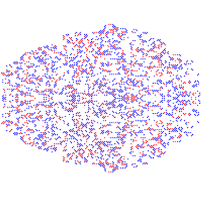
Figure 3: An example of a typical configuration generated by glider-supporting rules. Gliders multiply during collisions, so the whole space is filled by visually disorganized but in reality highly ordered pattern.

5 Quasi-chemical reaction

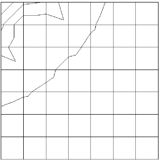
(a) $\mathbf{F}^{S}$

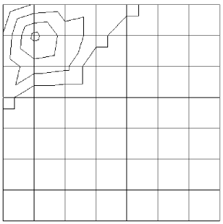
(b) $\mathbf{F}^{A}$

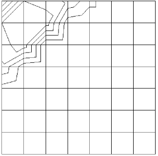
(c) $\mathbf{F}^{B}$

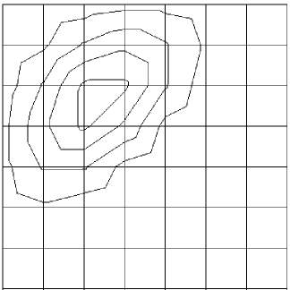
(d) $\mathbf{F}^{\#}$

Figure 4: Isolines representation for glider likehood matrices. Number of states of reactant $A$ increases from top left corner to bottom left, number of states of reactant $B$ increases from top left corner to top right one. In each case there is a single elevation. Approximate locations of elevations are $F_{00}^{S}$, $F_{11}^{A}$, $F_{11}^{B}$, and $F_{22}^{\#}$.

In order to characterize sets of possible quasi-chemical reactions, which lead to the formation of stationary and mobile perturbations of reagent concentrations, we provide isoline representation of the glider likehood matrices in Fig. 4. Based on the distributions shown in Fig. 4 we can speculate that

Finding 1

A probability, or rate, of dissociation of reactants decreases with the increase of number of the reactant molecules in each one local site of the medium.

See topology of isolines in Fig. 4a.

Finding 2

Reactions leading to production of reactants $A$ and $B$ are most likely to involve not more then four (usually between one and three) molecules of the reactants.

Distributions shown in Fig. 4a and b reach their ground-zero levels (no reaction take place) for the sites where satisfying the condition: Sum of molecules $A$ and molecules $B$ does not exceed four.

Finding 3

Reactant $B$ is more likely to be produced during quasi-chemical reactions derived from $\mathbf{F}$-matrices.

See Fig. 4a and b to compare area of elevations.

Basing on these findings we generalize glider likehood matrices to a set of abstract, quasi-chemical, reactions as follows:

$$\begin{matrix}A+B\stackrel{{\scriptstyle 1.}}{{\longrightarrow}}2A&\hskip 42.67912pt&A+2B\stackrel{{\scriptstyle 0.4}}{{\longrightarrow}}2A+B\cr 2A+B\stackrel{{\scriptstyle 0.1}}{{\longrightarrow}}3A&&2A+2B\stackrel{{\scriptstyle 0.01}}{{\longrightarrow}}3A+B\cr 3A+B\stackrel{{\scriptstyle 0.01}}{{\longrightarrow}}4A&&A+B\stackrel{{\scriptstyle 1.}}{{\longrightarrow}}2B\cr A+2B\stackrel{{\scriptstyle 0.1}}{{\longrightarrow}}3B&&2A+B\stackrel{{\scriptstyle 0.05}}{{\longrightarrow}}A+2B\cr B+S\stackrel{{\scriptstyle 0.01.}}{{\longrightarrow}}2B&&A\stackrel{{\scriptstyle 0.054}}{{\longrightarrow}}S\cr B\stackrel{{\scriptstyle 0.0015}}{{\longrightarrow}}S\cr&&\cr\end{matrix}$$ (1)

Figure 5: Concentration dynamics of $A$, $B$ and $S$ species in a well-stirred reactor. Simulated on CKS (Chemical Kinetics Simulator, IBM) with the following parameters: pressure and temperature are kept constant, volume is not tracked. 100K particles were simulated. Initial concentration of each species is 1 mole/l.

A typical scenario of how the system (1) behaves in a well-stirred reactor is shown in Fig. 5. We have confirmed in the computational experiments that the reaction scheme developed represents an oscillatory chemical system, where concentration of substrate is significantly higher than concentrations of reactants $A$ and $B$. This indeed conforms with the nature of spreading localizations and pulsating behavior of generators of localizations, or glider guns. The presence of both types of reactants in a localization is essential for the majority of propagating localisations, which is identified by the similarity of the dynamic of concentration profiles of reactants $A$ and $B$ shown in Fig. 5.

6 Reductions of transitions functions

What would be the behaviour of automata governed by the most likely cell-state transition rules? In order to find an answer we decided to reduce matrices of glider likehoods to their most articulated forms. First, we have made matrices more symmetrical by the following procedure. If $|F^{\prime}_{ij}-F^{\prime\prime}_{ji}|<\epsilon$ then we updated entries $(ij)$ and $(ji)$ as follows: $F^{\prime}_{ij}=F^{\prime\prime}_{ji}=\left\lfloor\frac{1}{2}(F^{\prime}_{ij}+F^{\prime\prime}_{ji})\right\rfloor$. We do this because we assume that in evolutionary experiments reactants $A$ and $B$ have the same diffusion coefficients.

Then we perform the following operation. If $|F^{A}_{ij}-F^{B}_{ij}|>0.2$ and $|F^{A}_{ij}-F^{S}_{ij}|>0.2$, or $F^{B}_{ij}=0$ and $F^{S}_{ij}=0$ then $M^{A}_{ij}=1$. We also discard entries of $(0,5)$ and $(1,4)$ of the matrix $M^{B}$ as being negligibly small, and omit the matrix $F^{\#}$ out of consideration. After these operation, we got the following matrix

$$\mathbf{R}=\begin{bmatrix}0&0&0&[0,1,2]&0&0&0&0\cr 0&1&[0,1,2]&0&0&0&0&\cr 0&[0,1,2]&[0,1]&0&0&0&&\cr[0,1,2]&[0,1]&0&0&0&&&\cr[0,1]&0&0&0&&&&\cr 0&0&0&&&&&\cr 0&0&&&&&&\cr 0&&&&&&&\cr\end{bmatrix}$$

where $R_{ij}$ is a set of all possible states that a cell $x$ can take if its neighbourhood $u(x)$ has $i$ cells in state $A$ and $j$ cells in state $B$. We found that

Finding 4

Starting its development from a random configuration a cellular automaton governed by a local transition functions expressed by matrix $\mathbf{R}$ exhibits still and breathing localizations.

Figure 6: Stationary localizations typically observed in automata governed by cell-state transition rules from class $\mathbf{R}$. State $A$ is shown by a circle, state $B$ by a solid disc.

Most common localizations observed in cellular automata with local transition rules from the class $\mathbf{R}$ are shown in Fig. 6. Minimal weight localizations are still triples of cells in state $A$ or $B$, or triples switching between $A$ and $B$ (Fig. 6a). These are followed by compact still patterns of four cells in $A$ or $B$ states, see examples in Fig. 6bc, switching compact patterns of four non-resting states Fig. 6d; and, wish-bone shaped clusters of $A$ and $B$ states Fig. 6e–h. The next heavier common localizations are the switching patterns of six Fig. 6i and eighth Fig. 6j non-resting states, and, the breathing localization Fig. 6k oscillating between 12 and 13 non-resting states.

7 Conclusion

We have hybridized the paradigm of reaction-diffusion cellular automata [4, 21, 5] with evolutionary techniques of breeding glider-supporting rules [13, 14, 15, 16] to statistically evaluate the set of all possible totalistic cell-state transition functions which support mobile and stationary localizations. We calculated exact structures of glider likehood matrices and interpreted them in terms of abstract reactions. We demonstrated that quasi-chemical systems derived from glider-supporting rules exhibit classical dynamics of excitable chemical systems. We obtained computational experiment evidences that by reducing glider likehood matrices to their strong components we obtain a set of local transition rules that exhibit exclusively stationary localizations. Results of the research undertaken provide a priceless tool for designing collision-based computing schemes in spatially extended non-linear systems.

References

- [1] Adamatzky A. New media for collision-based computing, In: Adamatzky A. (Ed.) Collision-Based Computing (Springer, 2003) 411-442.
- [2] Adamatzky A. (Ed.) Collision-Based Computing (Springer, 2003).
- [3] Adamatzky A. Collision-based computing in Belousov-Zhabotinsky medium, Chaos, Solitons & Fractals 21 (2004) 1259–1264.
- [4] Adamatzky A., Wuensche A. and De Lacy Costello B. Glider-based computing in reaction-diffusion hexagonal cellular automata. Chaos, Solitons & Fractals 27 (2006) 287–295.
- [5] Adamatzky A. and Wuensche A. Computing in spiral rule reaction-diffusion hexagonal cellular automaton, Complex Systems 16 (2007) 4.
- [6] Adamatzky A. Java applet on probabilistic selection of glider-supporting hexagonal cellular automata. 2007. http://uncomp.uwe.ac.uk/adamatzky/erdca/
- [7] Berlekamp E., Conway J. and Guy R. Winning Ways, vol. 2, (Academic Press, 1982).
- [8] Chazottes J.-R. and Fernandez B. (Eds.) Dynamics of Coupled Map Lattices and of Related Spatially Extended Systems (Springer-Verlag, 2005).
- [9] De Lacy Costello B. and Adamatzky A. Experimental implementation of collision-based gates in Belousov-Zhabotinsky medium, Chaos, Solitons and Fractals (2005).
- [10] Fredkin E. and Toffoli T. Conservative logic Int. J. Theor. Phys. 21 (1982) 219–253.
- [11] Liehr, A. W.; Bode, M.; Purwins, H.-G.: The Generation of Dissipative Quasi-Particles near Turing’s Bifurcation in Three-Dimensional Reaction-Diffusion-Systems. In: Krause, E.; J ger, W. (Hrsg.): High Performance Computing in Science and Engineering 2000. Transactions of the High Performance Computing Center, Stuttgart (HLRS) 2000, Springer, 2001, S. 425–439.
- [12] Margolus N. Physics–like models of computation. Physica D 10 (1984) 81–95.
- [13] Sapin E., Bailleux O., and Chabrier J.J.. Research of a cellular automaton simulating logic gates by evolutionary algorithms. Lecture Notes in Computer Science, 2610 (2003) 414- 423.
- [14] Sapin E., Bailleux O., and Chabrier J.J. Research of complex forms in the cellular automata by evolutionary algorithms. Lecture Notes in Computer Science 2936 (2003) 357–367.
- [15] Sapin E., Bailleux O., Chabrier J.J. and Collet P. A new universal cellular automaton discovered by evolutionary algorithms. Lecture Notes in Computer Science 3102 (2004) 175–187.
- [16] Sapin E., Bailleux O., Chabrier J. J. and Collet P. Demonstration of the universality of a new cellular automaton. Int. J Unconventional Computing 3 (2007) 79–103.
- [17] Sediña-Nadal I., Mihaliuk E., Wang J., Pérez-Muñuzuri W. and Showalter K., Wave propagation in subexcitable media with periodically modulated excitability. Phys. Rev. Lett. 86 (2001) 1646.
- [18] Soukoulis C.M. (Ed.) Photonic Crystals and Light Localization in the 21st Century: Proceedings of the NATO Advanced Study Institute on Photonic Crytals and Light Localization (Kluwer Academic Publishers, 2001)
- [19] Vakakis A. (Ed.) Normal Modes and Localization in Nonlinear Systems (Kluwer Academic Publishers, 2001)
- [20] Wuensche A. Glider dynamics in 3-value hexagonal cellular automata: the beehive rule. Int. J. of Unconventional Computing 1 (2005) 375–398.
- [21] Wuensche A. and Adamatzky A. On spiral glider-guns in hexagonal cellular automata: activator-inhibitor paradigm. Int J Modern Physics C 17 (2006) 1009-1026.