Classical Spin Models with Broken Continuous Symmetry: Random Field Induced Order and Persistence of Spontaneous Magnetization

Abstract

We consider a classical spin model, of two-dimensional spins, with continuous symmetry, and investigate the effect of a symmetry breaking unidirectional quenched disorder on the magnetization of the system. We work in the mean field regime. We show, by numerical simulations and by perturbative calculations in the low as well as in the high temperature limits, that although the continuous symmetry of the magnetization is lost, the system still magnetizes, albeit with a lower value as compared to the case without disorder. The critical temperature at which the system starts magnetizing, also decreases with the introduction of disorder. However, with the introduction of an additional constant magnetic field, the component of magnetization in the direction that is transverse to the disorder field increases with the introduction of the quenched disorder. We discuss the same effects also for three-dimensional spins.

I Introduction

Disordered systems, both classical and quantum, lie at the center-stage of condensed matter physics booksondisorder ; amrasobai . Challenging open questions in disordered systems include those in the realms of spin glasses spinglass , neural networks nn , percolation percolation , and high $T_{c}$ superconductivity superconduc . Phenomena like Anderson localization Anderson ; booksonanderson , and absence of magnetization in several classical spin models imryma1 ; imryma2 ; janek are effects of disorder.

In particular, classical ferromagnetic spin models with discrete, or continuous, symmetries are very sensitive to random magnetic fields, distributed in accordance with the symmetry, in low dimensions imryma1 . For instance, an arbitrary small random magnetic field with $Z_{2}$ ($\pm$) symmetry destroys spontaneous magnetization in the Ising model in 2D at any temperature $T$, including $T=0$. Similar effect holds for the XY model in 2D at $T=0$ in a random field with $U(1)$ ($SO(2))$ symmetry, or Heisenberg model in 2D at $T=0$ in $SU(2)$ ($SO(3)$) symmetry in random field. In these cases, the effects of disorder amplify the effects of continuous symmetry, that destroys spontaneous magnetization at any $T>0$. The effect is even more dramatic in 3D, where the random field destroys spontaneous magnetization at any $T\geq 0$. (For a general description of these, see imryma1 ; imryma2 ; janek .)

The appropriate symmetry of the random field is essential for the above mentioned results. The natural question arises as to what happens if the distribution of the random field does not exhibit the symmetry, in particular the continuous symmetry. Yet another natural question is how does the spin systems in random fields behave in the quantum limit. The latter question is particularly interesting in view of the fact that nowadays it is possible to realize practically ideal models of quantum spin systems (with spin s=1/2, 1, 3/2, …, and with Ising, XY, or Heisenberg interactions) in controlled random fields amrasobai ; Armand . It is therefore very important to understand the physics of both classical and quantum spin models in random fields that break their symmetry.

In this paper, we will consider the classical XY spin model in a random field that breaks the continuous U(1) ($SO(2)$) symmetry. We investigate this model in the mean field approximation mean . Despite its simplicity, this model with the two-dimensional spin variable, magnetizes in the absence of disorder below a certain critical temperature, which can be calculated exactly. As a result of continuous symmetry, the possible values of spontaneous magnetization form a circle in the plane. A random magnetic field pointing along the $Y$-direction is introduced, by adding a new term to the energy of the model. This term breaks the continuous symmetry of the model, but the critical temperature persists. The present paper studies the critical behaviour and properties of spontaneous magnetization in the resulting mean-field disordered system. We prove that, as may be expected, adding a random field lowers the critical temperature. Next, we show that the magnetization of the disordered system is lower than that of the pure one—another intuitively plausible result, first shown numerically and then by perturbation expansions: one around the critical temperature of the pure model and another for low temperatures.

Next, we introduce a constant magnetic field, which breaks the continuous symmetry of the model even in the absence of disorder. In fact, the system now magnetizes at all temperatures in the direction parallel to the magnetic field. When we now also add a random field as described above, the length of the magnetization vector decreases again. Moreover, the magnetization gets atrracted towards the $X$- axis, i.e. the direction transverse to that of the random field. However, the $X$-component of the magnetization can increase for certain choices of the constant field. We view this effect as a case of “random field induced order”, by analogy with the effect studied in Armand , where numerical evidence was given for appearance of magnetization in the XY model on a two-dimensional lattice with the introduction of disorder. In contrast to the present work, in this other case no mean-field approximation was used and no uniform magnetic field was introduced.

The effect of “random field induced order” has, of course, a long history history . Recently it has become vividly discussed in the context of $XY$ ordering in a graphene quantum Hall ferromagnet lee , and ordering in $\phantom{i}{}^{3}$He-A arerogel and amorphous ferromagnets fomin . Let us stress that the novel aspects of our previous paper Armand consists in clarifying certain aspect of the rigorous proof of the appearance of magnetization in XY model at $T=0$, presentation of a novel evidence for the same effect at $T>0$, and a proposal for realisation of quantum version of the effect with ultracold atoms. In the subsequent paper Armand2 , we have shown how the “random field induced order” exhibits itself in a system of two-component trapped Bose-Einstein condensate with random Raman inter-component coupling. The novelty of the present paper lies in systematic mean field treatment of the disordered $XY$ model with particular emphasis on the response to the constant magnetic field.

The paper is arranged as follows. In Sect. II the ferromagnetic XY model is introduced. A symmetry breaking random field is added in Sect. III and the results of numerical simulations of and perturbative calculations on the resulting model are presented. In Sect. IV, study the system with an additional constant field and, in particular, show presence of random field-induced order. We discuss the results in Sect. V, arguing in particular that the analogs of our results will hold for the mean-field version of the classical Heisenberg model.

II Ferromagnetic XY model: Mean Field approach

Consider a lattice, each site $i$ of which is occupied by a “spin”, which is a unit vector $\vec{\sigma}_{i}=(\cos\theta_{i},\sin\theta_{i})$ on a two-dimensional plane (called the XY plane). The nearest-neighbor ferromagnetic XY model is defined by the Hamiltonian

$$H_{XY}=-J\sum_{|i-j|=1}{\vec{\sigma_{i}}}\cdot\vec{\sigma_{j}},$$ (1)

with a coupling constant $J>0$. This model does not have any spontaneous magnetization, at any temperature, in one and two dimensions (Mermin-Wagner-Hohenberg theorem Mermin-Wagner ), while a finite magnetization appears in higher dimensions for sufficiently low temperatures spinwave ; Frohlich .

Let us assume that the total number of spins in our system is $N$. In the mean field approximation every spin is assumed to interact with all other spins (not just with the nearest neighbors) with the same coupling constant $-J$. Therefore, the contribution of the spin at $i$ to the total energy of the system equals

$$\left(-{J\over N}\sum_{j:j\neq i}\vec{\sigma}_{j}\right)\cdot\vec{\sigma}_{i},$$

where we divided the energy term by $N$ in order to preserve its order of magnitude. This effective interaction, replacing the nearest neighbor interaction in $H_{XY}$, is for large $N$ approximately equal

$$\frac{1}{N}\left(-J\sum_{j}{\vec{\sigma_{j}}}\right)\cdot{\vec{\sigma_{i}}}$$

$$= -J{\vec{m}}\cdot{\vec{\sigma_{i}}},$$ (2)

where ${\vec{m}}=\frac{1}{N}\sum_{i=1}^{N}\vec{\sigma}_{i}$. The mean field approximation consists of treating $\vec{m}$ as a genuine constant vector and adjusting it so, that the canonical average of the spin at (any) site $i$ equals this constant. If the system is in canonical equilibrium at temperature $T$, the average value of the spin vector $\vec{\sigma}_{i}$ is

$$\langle{\vec{\sigma_{i}}}\rangle=\frac{\int{\vec{\sigma}_{i}}\exp(\beta J{\vec{m}}\cdot{\vec{\sigma}_{i}})d{\vec{\sigma}_{i}}}{\int\exp(\beta J{\vec{m}}\cdot{\vec{\sigma}_{i}})d{\vec{\sigma}_{i}}},$$ (3)

where $\beta=1/(k_{B}T)$, with $k_{B}$ being the Boltzmann constant. This average is independent of the site $i$. Consistency requires that the left hand side (l.h.s.) of the above equation be equal to the magnetization ${\vec{m}}$. Hence, we obtain the mean field equation

$${\vec{m}}=\frac{\int{\vec{\sigma}}\exp(\beta J{\vec{m}}\cdot{\vec{\sigma}})d{\vec{\sigma}}}{\int\exp(\beta J{\vec{m}}\cdot{\vec{\sigma}})d{\vec{\sigma}}},$$ (4)

where we have dropped the index $i$. Equations of this type, for various modifications of the original interaction are the main subject of this work.

Let

$${\vec{m}}=(m\cos a,m\sin a).$$ (5)

For sufficiently high temperatures, the only solution fo the mean field equation is $\vec{m}=0$. There exists a $\beta_{c}^{0}$, such that for $\beta>\beta_{c}^{0}$, this system magnetizes. (Later, we will consider the case of a system with an additional quenched disordered field of strength $\epsilon$. The superscript of $\beta_{c}^{0}$ is anticipation of that case.) By symmetry, the solutions of the above mean field equation (Eq. (4)) form a circle

$$|{\vec{m}}|=m_{0},$$ (6)

with a strictly positive radius $m_{0}$, for any $\beta>\beta_{c}^{0}$. Choosing the phase $a=0$, Eq. (4) reduces to

$$m=\frac{\int_{0}^{2\pi}\cos\theta\exp(\beta Jm\cos\theta)d\theta}{\int_{0}^{2\pi}\exp(\beta Jm\cos\theta)d\theta},$$ (7)

where we have taken

$$\vec{\sigma}=(\cos\theta,\sin\theta).$$ (8)

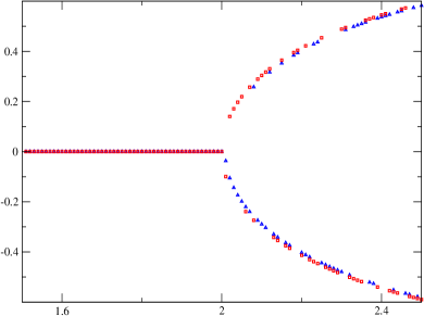
Figure 1: (Color online.) The behavior of magnetization (vertical axis) with respect to $\beta J$ (horizontal axis). The (red) squares represent the magnetization of the XY model without disorder (the corresponding Hamiltonian being $H_{XY}$), while the (blue) traingles are that for the same, but with disorder (the corresponding Hamiltonian being $H_{\epsilon}$ with $\epsilon=0.1$).

In Fig. 1, the red squares represent the cross-section, of the surface of solutions of Eq. (4) in the $(m\cos a,m\sin a,\beta)$ Cartesian space, in the $\cos a=0$ plane.

From numerical simulations (see Fig. 1), we found that $\beta_{c}^{0}J\approx 2.00$. One can show analytically that $\beta_{c}^{0}J$ is exactly 2, as follows. Let us denote the right hand side (r.h.s.) of Eq. (7) by $F(m)$. The condition for the system to magnetize, for a given value of $\beta$, is that the derivative of the r.h.s. of Eq. (7) at $m=0$, i.e. $F^{{}^{\prime}}(m){|}_{m=0}$ should be greater than the derivative of the l.h.s. It is easy to check that

$$F^{{}^{\prime}}(m){|}_{m=0}=\beta J/2.$$

This implies that the system possesses a nonzero magnetization, if and only when

$$\beta>2/J=\beta_{c}^{0}.$$

III Ferromagnetic XY model in a random field

We will now consider the effect of additional quenched random fields. Let us begin by reminding the notions of quenched disorder and quenched averaging.

III.1 Quenched averaging

The disorder considered in this paper is “quenched”, i.e. its configuration remains unchanged for a time that is much larger than the duration of the dynamics considered. In the systems that we study, it is the local magnetic fields that are disordered. They are random variables following certain probability distributions. Since the disorder is quenched, a particular realization of all the random variables remains fixed for the whole time necessary for the system to equilibrate. An average of a physical quantity, say $A$, is thus to be carried out in the following order.

• Compute the value of the physical quantity $A$, with the fixed configuration of the disorder.

• Average over the disordered parameters.

This mode of averaging is called “quenched” averaging. It may be mentioned that an averaging in which items (a) and (b) are interchanged in order, is called “annealed” averaging. Physically it corresponds to a situation when the disorder fluctuates on time scales comparable to the system’s thermal fluctuations.

III.2 The model and the mean field equation for magnetization

The $XY$ model with an inhomogeneous magnetic field has the interaction:

$$H=-J\sum_{|i-j|=1}\vec{\sigma_{i}}\cdot\vec{\sigma_{j}}-\epsilon\sum_{i}\vec{h}_{i}\cdot\vec{\sigma}_{i}.$$ (9)

where the two-dimensional vectors $\vec{h}_{i}$ are the external magnetic fields, up to a coefficient $\epsilon$. In the sequel $\vec{h}_{i}$ are random variables of order one, they model the disorder in the system and thus $\epsilon$ measures the disorder’s strength. More precisely, let $\vec{h}_{i}$ be independent and identically distributed random variables (vector-valued). We want to study the effect of including such a random field term in the $XY$ hamiltonian at small values of $\epsilon$. As argued in Armand , in lattice $XY$ models this effect depends critically on the properties of the probability distribution of the random fields.

If the distribution of the $\vec{h}_{i}$ is invariant under rotations, there is no spontaneous magnetization at any nonzero temperature in any dimension $d\leq 4$. imryma1 ; imryma2 ; janek

We now want to see the effect of a random field that does not have the rotational symmetry of the XY model interaction (1), considering the case when

$$\vec{h}_{i}=\eta_{i}\cdot\vec{e}_{y}$$ (10)

where $\eta_{i}$ are scalar random variables with a distribution symmetric about $0$ and $\vec{e}_{y}$ denotes the unit vector in the $y$ direction. The main result of Armand is that on the two-dimensional lattice such a random field will break the continuous symmetry and the system will magnetize, even in two dimensions, thus destroying the Mermin-Wagner-Hohenberg effect. Above two dimensions the pure $XY$ model magnetizes at low temperatures and it has been suggested in Armand that the uniaxial random field as described above may enhance this magnetization. In the present paper we want to study related effects at the level of a simpler, mean-field model, which allows for a more detailed analysis and more accurate simulations.

We consider the mean-field Hamiltonian given by

$$H_{\epsilon}=-J\vec{m}\cdot\vec{\sigma}-\epsilon\vec{\eta}\cdot{\vec{\sigma}},$$ (11)

where, as $\vec{\eta}_{i}$ before,

$$\vec{\eta}=\eta\cdot\vec{e}_{y}$$

is the quenched random field in the $y$-direction. Here $\eta$ is a scalar, symmetric random variable, which we assume here to be Gaussian distributed with zero mean and unit variance. $\epsilon$ $(>0)$ is the parameter (typically small) that quantifies the strength of the randomness.

The corresponding mean field equation for magnetization is:

$${\vec{m}}=Av_{\eta}\left[\frac{\int{\vec{\sigma}}\exp(\beta J{\vec{m}}\cdot{\vec{\sigma}}+\beta\epsilon\eta\sigma_{y})d{\vec{\sigma}}}{\int\exp(\beta J{\vec{m}}\cdot{\vec{\sigma}}+\beta\epsilon\eta\sigma_{y})d{\vec{\sigma}}}\right].$$ (12)

Here $Av_{\eta}(\cdot)$ denotes the average over the disorder, i.e. the integral over $\eta$ with the appropriate distribution (here assumed to be unit normal).

III.3 Numerical simulations

It follows from the symmetry of the distribution of $\eta$ that all solutions of the equation (Eq. (12)) have zero $Y$-component. In the case of $\epsilon\neq 0$, the system again does not magnetize at high temperature, as in the case of $\epsilon=0$. However, there exists a critical temperature, below which a transverse (with respect to the direction of the random field) magnetization appears. More precisely, there exists a $\beta_{c}^{\epsilon}$ such that for $\beta>\beta_{c}^{\epsilon}$, the magnetization equation has two solutions with zero $Y$-components, whose $X$-components equal $m$ and $-m$ (where $m>0$) (along with the trivial solution $m=0$). We will study the dependence of $m$ on the temperature and on the disorder strength $\epsilon$. Therefore, in contrast to the continuous set (a circle) of solutions of the mean field equation in the system without disorder (modelled by $H_{XY}$), in the disordered case there are just two possible values of the spontaneous magnetization. In Fig. 1, the blue triangles represent the magnetization for $\epsilon=0.1$, while the red squares correspond to $\epsilon=0$. The same color code applies to Fig. 2, where, in addition, pink stars represent the case $\epsilon=0.15$, and green circles—$\epsilon=0.2$. All the curves show two real solutions ($m$ and $-m$), of the corresponding mean field equation, at low temperatures. From Figs. 1 and 2, it is clear that $m(\beta,\epsilon)$ is smaller than $m_{0}$ (see Eq. (6)), at low temperatures. They coincide for high temperatures, as both of them are vanishing in that regime. Numerical simulations show that the difference $\delta(\beta,\epsilon)=m_{0}-m(\beta,\epsilon)=m(\beta,0)-m(\beta,\epsilon)>0$ is of the order of $\epsilon^{2}$, in the regime of $\beta>\beta_{c}^{\epsilon}$ (see Fig. 2).

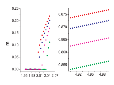
Figure 2: (Color online.) The magnetization ($m$) with respect to $\beta J$ (horizontal axes): the (red) squares, (blue) triangles, (pink) stars, and (green) circles are for the system described by the Hamiltonian $H_{\epsilon}$ with $\epsilon=0$, $\epsilon=0.1$, $\epsilon=0.15$, and $\epsilon=0.2$ respectively. The figure on the left correspond to the behavior of the spontaneous magnetization near the critical temperature, while that on the right correspond to the same at lower temperatures. The decrease of magnitude of the magnetization due to disorder, is clearly of the order of $\epsilon^{2}$.

III.4 Scaling of critical temperature and magnetization with disorder: Perturbative approach

In this subsection, we will study the mean field Hamiltonian in Eq. (11), using perturbation theory and compare the results with the numerical results of the last section. Since, as argued earlier, the spontaneous magnetization can only have nonzero $X$-component at any temperature, the mean field equation (Eq. (12)) reduces to

$$m=Av_{\eta}\left[\frac{\int_{0}^{2\pi}\cos\theta\exp(\beta Jm\cos\theta+\beta\epsilon\eta\sin\theta)d\theta}{\int_{0}^{2\pi}\exp(\beta Jm\cos\theta+\beta\epsilon\eta\sin\theta)d\theta}\right]$$

$$\equiv F_{\epsilon}(m).$$ (13)

Note that $F_{\epsilon}(m)=F(m)$ for $\epsilon=0$.

III.4.1 Critical temperature

To find the critical temperature, a similar method as in the case of $\epsilon=0$ (in the preceding section) is applied. The condition for non-zero magnetization is now given by

$$F^{{}^{\prime}}_{\epsilon}(0)=\frac{\beta J}{2}-\frac{\beta^{3}\epsilon^{2}J}{16}+o(\epsilon^{2})>1,$$ (14)

where $o(\zeta^{n})$ denotes a term which is of order higher than $\zeta^{n}$. This implies

$$\beta_{c}^{\epsilon}=\beta_{c}^{0}-\frac{\epsilon^{2}}{2J^{3}}+o(\epsilon^{2}).$$ (15)

Therefore, we obtain negative $\epsilon^{2}$ corrections to the critical temperature, as observed in the numerical simulations (see Fig. 2).

III.4.2 Scaling of magnetization near criticality

The magnetization goes to zero as the temperature approaches the critical temperature. Let us now use perturbation techniques to see the behavior of magnetization $m$ near criticality.

Before considering the disordered case ($\epsilon\neq 0$), let us first consider the case when $\epsilon=0$. In this case, we expand $F(m)$ (r.h.s. of Eq. (7)) in $m$ around $m=0$:

$$F(m)=mF^{{}^{\prime}}(0)+\frac{m^{3}}{6}F^{{}^{\prime\prime\prime}}(0)+\mbox{higher order terms}.$$ (16)

Differentiating Eq. (4) and considering the resulting elementary integrals one can easily see that, by symmetry, $F(0)=F^{{}^{\prime\prime}}(0)=0$ and that

$$F^{{}^{\prime}}(0)=\beta J/2,\quad F^{{}^{\prime\prime\prime}}(0)=-3\beta^{3}J^{3}/8.$$ (17)

Putting these values in Eq. (16), we obtain that the magnetization near $\beta_{c}^{0}$ equals

$$m_{0}=\frac{2\sqrt{2}}{J}\beta^{-\frac{3}{2}}(\beta-\beta_{c}^{0})^{\frac{1}{2}}.$$ (18)

plus higher order terms.

A similar technique can now be used to study the behavior of $m$ near $\beta_{c}$ in the presence of disorder. Again $F_{\epsilon}(0)=F^{{}^{\prime\prime}}_{\epsilon}(0)=0$. Hence the expansion of $F_{\epsilon}(m)$ near zero will be

$$F_{\epsilon}(m)=mF^{{}^{\prime}}_{\epsilon}(0)+\frac{m^{3}}{6}F^{{}^{\prime\prime\prime}}_{\epsilon}(0)+\mbox{higher order terms},$$ (19)

where

$$F^{{}^{\prime}}_{\epsilon}(0) = \left(\frac{\beta J}{2}-\frac{\beta^{3}\epsilon^{2}J}{16}\right),$$

$$F^{{}^{\prime\prime\prime}}_{\epsilon}(0) = \beta^{3}J^{3}\left[\left(\frac{3}{8}-\frac{\beta^{2}\epsilon^{2}}{32}\right)-3\left(\frac{1}{2}-\frac{\beta^{2}\epsilon^{2}}{16}\right)^{2}\right]$$

Putting these derivatives in Eq. (19), we obtain the correction of magnetization due to disorder as

$$m=m_{0}\left(1-\frac{1}{2J^{2}m_{0}^{2}}\epsilon^{2}+o(\epsilon^{2})\right).$$

This is in full agreement with numerical simulations, that also showed a decrease of magnetization of order $\epsilon^{2}$, in the disordered case, as compared to the case when $\epsilon=0$.

III.4.3 A modified Bessel function and its expansion for large arguments

In the following, we will have numerous occasions to use the modified Bessel function

$$I_{n}(z)=\frac{1}{\pi}\int_{0}^{\pi}\exp(z\cos\vartheta)\cos(n\vartheta)d\vartheta,$$ (20)

where $n$ is an integer, and $z$ is a real number, and the expansion of $I_{n}(z)$ for large $|z|$: Abrohamawitz

$$I_{n}(z) \approx \frac{\exp(z)}{\sqrt{2\pi z}}\Big{[}1-\frac{\mu-1}{8z}+\frac{(\mu-1)(\mu-9)}{2!(8z)^{2}}$$

$$-\frac{(\mu-1)(\mu-9)(\mu-25)}{3!(8z)^{3}}+o\left(\left(1/z\right)^{3}\right)\Big{]},$$

where $n$ is fixed and $\mu=4n^{2}$. Actually, the function and its expansion are true Abrohamawitz for certain complex ranges of the parameter $z$. However, we will only use them for real $z$. Here $o\left(\left(1/\upsilon\right)^{n}\right)$ denotes an expression, containing terms of order higher than $({1\over n})^{n}$: $\left(1/\upsilon\right)^{n+1},\left(1/\upsilon\right)^{n+2},\ldots$.

III.4.4 Scaling of magnetization at low temperature

We now study behavior of $m$ at low temperatures, i.e. for large $\beta$.

We again start from the case $\epsilon=0$. Note that the numerator and denominator of $F(m)$ (after some simple modifications) are of the form of $I_{n}(z)$. Therefore, for large $\beta$, we can use the asymptotics of the Bessel function in Eq. (III.4.3) to obtain a low temperature expansion of $F(m)$. Using this expansion, we obtain the following equation for $m$, from Eq. (7):

$$m^{3}-m^{2}+\frac{m}{2\beta J}+o\left(1/\beta\right)=0.$$ (22)

Since $m\rightarrow 1$ as $\beta\rightarrow\infty$, let us write $m$ as

$$m=1-\frac{a_{1}}{\beta}+o\left(1/\beta\right).$$ (23)

Putting this in Eq. (22), we finally obtain the behavior of the magnetization for the case when $\epsilon=0$, for large $\beta$:

$$m_{0}=1-\frac{1}{2J\beta}+o\left(1/\beta\right).$$ (24)

Using the same technique for the disordered case, we expand the numerator and denominator of $F_{\epsilon}(m)$, using Eq. (III.4.3), obtaining

$$m = 1-\frac{\epsilon^{2}}{2J^{2}}-\frac{1}{\beta}\left[\frac{1}{2J}+\epsilon^{2}\left(\frac{3}{4J^{3}}-\frac{1}{2J^{2}}\right)\right]+o(1/\beta)$$

$$= m_{0}-\epsilon^{2}\left\{\frac{1}{2J^{2}}+\frac{1}{\beta}\left[\left(\frac{3}{4J^{3}}-\frac{1}{2J^{2}}\right)\right]\right\}+o(1/\beta).$$

As before, disorder leads to corrections of order $\epsilon^{2}$ to the magnetization at low temperature. This is again in agreement with the numerical simulations (see Fig. 2).

IV Ferromagnetic XY model in a random field plus a constant field: Random field induced order

We have seen in the preceding section that a random field that breaks the symmetry of the XY model, restricts possible magnetization values to a discrete set. Although the system still magnetizes, we no longer have continuously symmetry of the set of solutions to the mean field equation, as a result of adding a symmetry-breaking random field. In this section we explore the effects of such a random field on a system which already has a unique direction of the magnetization, determined by a uniform magnetic field.

First consider the case in which the planar symmetry in the XY model is broken by applying a constant magnetic field $\vec{h}$ alone. That is, according to the general mean field strategy, we are looking for the solutions of the following equation:

$${\vec{m}}=\frac{\int{\vec{\sigma}}\exp(\beta J{\vec{m}}\cdot{\vec{\sigma}}+\beta{\vec{h}}\cdot{\vec{\sigma}})d{\vec{\sigma}}}{\int\exp(\beta J{\vec{m}}\cdot{\vec{\sigma}}+\beta{\vec{h}}\cdot{\vec{\sigma}})d{\vec{\sigma}}}.$$ (26)

Let ${\vec{h}}=(h\cos x,h\sin x)$. We suppose that $0<h\leq 1$ and $0\leq x\leq\pi/2$. As expected, due to the applied constant field, the mean field equation has a unique solution of the magnetization $\vec{m}$ at all temperatures, and the solution is a (positive) multiple of ${\vec{h}}$, but of reduced magnitude. Red squares in Figs. 5, 3, 6, and 4, correspond to the magnitude ($m$) and the cosine of the phase ($a$) of the magnetization $\vec{m}$.

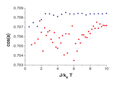
Figure 3: (Color online.) Plot of $\cos(a)$ with respect to $\beta J$. Red squares represent the case when the XY model has the applied constant field $\vec{h}$ with $h=J$ and $x=\pi/4$. Blue triangles are for the same system but with the additional symmetry breaking random field of strength $\epsilon=0.1J$.

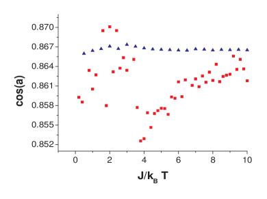
Figure 4: (Color online.) This is the same plot as in Fig. 3, but for $x=\pi/6$.

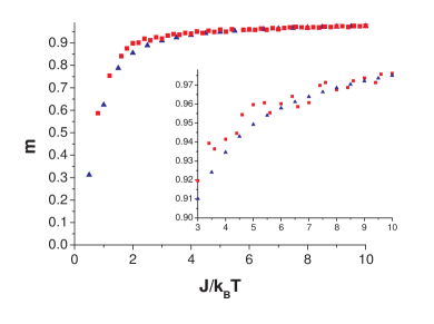
Figure 5: (Color online.) Plot of the magnitude $m$ of the magnetization with respect to $\beta J$. Red squares represent the case when the XY model has the applied constant field $\vec{h}$ with $h=J$ and $x=\pi/4$. Blue triangles are for the same system but with the additional symmetry breaking random field of strength $\epsilon=0.1J$.

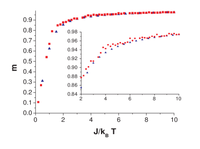
Figure 6: (Color online.) This is the same plot as in Fig. 5, but for $x=\pi/6$.

Let us now, in addition, apply a random field $\{\eta\}$ in the Y-direction. The new mean field equation is

$${\vec{m}}=Av_{\eta}\left[\frac{\int{\vec{\sigma}}\exp(\beta J{\vec{m}}\cdot{\vec{\sigma}}+\beta{\vec{h}}\cdot{\vec{\sigma}}+\beta\epsilon\eta\sigma_{y})d{\vec{\sigma}}}{\int\exp(\beta J{\vec{m}}\cdot{\vec{\sigma}}+\beta{\vec{h}}\cdot{\vec{\sigma}}+\beta\epsilon\eta\sigma_{y})d{\vec{\sigma}}}\right].$$ (27)

Here we have to solve the two simultaneous equations, given by Eq. (27), to obtain the magnitude and the phase of the magnetization vector $\vec{m}$. In all the previous mean field (vector) equations, one could apriori predict the phase of the magnetization. Just as in the case of a constant field $\vec{h}$ and $\epsilon=0$, again the solution remains unique.

Just as in the previous sections, we will now compare the magnetization of the system without disorder (i.e. $\epsilon=0$, and for which the mean field equation is given by Eq. (26))), with the system in which $\epsilon\neq 0$ (and for which the mean field equation is given by Eq.(27))keeping $h$ strictly positive in both cases. Let us denote the two Hamiltonians by $H_{h}$ and $H_{h,\epsilon}$ respectively. We do the comparison by numerical simulations as well as perturbatively at low temperatures (Sect. IV.1 below). A perturbation approach, similar to the one in Sect. III.4.2, can be done at high temperatures also. We refrain from doing it, as the high temperature behavior in this case is not so interesting, in view of absence of a phase transition.

The length $m$ of the magnetization vector is shrunk inthe system described by $H_{h,\epsilon}$, compared to the case in which there is no disorder in the system (i.e. the one described by $H_{h}$). This is seen from numerical simulations (see Figs. 5 and 6), as well as by perturbation techniques at low temperatures. In addition, numerical simulations (as shown in Figs. 3 and 4) show that the cosine of the phase of the magnetization, i.e. $\cos(a)$ increases in presence of the random field. Therefore, the phase of the magnetization vector moves towards the X-direction (i.e. the direction transverse to the applied random field). This is also corroborated by perturbative approach at low temperatures. The schematic diagram in Fig. 7 shows the change of behavior of the length and phase of the magnetization with and without disorder, in the presence of a constant field.

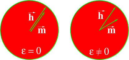
Figure 7: (Color online.) Schematic diagram of the magnetization of XY ferromagnets without and with disorder, in the presence of a constant magnetic field. The figure on the left indicates the behavior of $\vec{m}$ in the presence of $\vec{h}$, but when $\epsilon=0$, while the one on the right is when there is a positive $\epsilon$.

The $Y$-component, $m_{y}=m\sin a$, of the magnetization has the same relative behavior as the length $m$, in systems described by $H_{h}$ and $H_{h,\epsilon}$, i.e. for small $\epsilon>0$ it is lower than for $\epsilon=0$.

However, the $X$-component, $m_{x}=m\cos a$, of the magnetization, $\vec{m}$, behaves in a very interesting way. Its value in the system described by $H_{h,\epsilon}$ can be both higher as well as lower than its value in the system described by $H_{h}$. The numerical simulations in this case are given in Fig. 8.

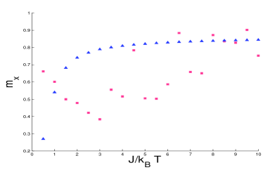
Figure 8: (Color online.) Order from disorder: Red squares are the X-components of the magnetization in the absence of disorder, while blue triangles are those in the presence of disorder $\epsilon=0.1J$. The constant field is present in both cases, with $x=\pi/6$.

IV.1 Magnetization at low temperature: Perturbative approach

To obtain the behavior of magnetization at low temperature, we will use the implicit function theorem, which we now state. Let an equation $f(x_{1},x_{2})=0$ of two variables $x_{1}$ and $x_{2}$ be such that $f(x_{1},x_{2})=0$ at $(x_{1},x_{2})=(x_{1}^{0},x_{2}^{0})$. $x_{2}$ is in general an unknown function of $x_{1}$. But we may still understand the character of $\frac{dx_{2}}{dx_{1}}|_{x_{1}=x_{1}^{0}}$, by using the fact that (under certain regularity conditions on $f$ near $(x_{1}^{0},x_{2}^{0})$)

$$\frac{\partial f}{\partial x_{1}}\Big{|}_{(x_{1}^{0},x_{2}^{0})}+\frac{\partial f}{\partial x_{2}}\Big{|}_{(x_{1}^{0},x_{2}^{0})}\frac{dx_{2}}{dx_{1}}\Big{|}_{(x_{1}^{0},x_{2}^{0})}=0.$$ (28)

The usual statement of the implicit function theorem is that when ${\partial f\over\partial x_{2}}$ is nonzero at $(x_{1}^{0},x_{2}^{0})$), we can solve the equation $f(x_{1},x_{2})=0$ for $x_{2}$ uniquely near this point and the derivative of the resulting function ($x_{2}$ as a function of $x_{1}$) at $x_{1}^{0}$ can then be calculated from the above equation. However, in the case when the first derivatives vanish at a certain point, we can use a simple extension of it to calculate the second derivatives. Such a situation appears in the calculations below of the second derivatives of the magnetization with respect to $\epsilon$.

The mean field equations that we work with here can be written in the form

$$\vec{m}=\frac{1}{\beta J}\nabla_{\vec{m}}\Gamma,$$ (29)

where

$$\nabla_{\vec{m}}\equiv\left(\frac{\partial}{\partial m_{x}},\frac{\partial}{\partial m_{y}}\right),$$ (30)

with

$$\Gamma=\log_{e}\int\exp\left(-\beta H_{h}\right)\quad\mbox{or}\quad\log_{e}\int\exp\left(-\beta H_{h,\epsilon}\right).$$ (31)

It follows from symmetry of the distribution of $\eta$ that $\vec{m}$ is an even function of $\epsilon$ and, consequently $\frac{dm_{x}}{d\epsilon}$ and $\frac{dm_{y}}{d\epsilon}$ vanish at $\epsilon=0$.

It follows that

$$\frac{d^{2}m_{x}}{d\epsilon^{2}}\left[1-\frac{1}{\beta J}\frac{\partial^{2}\Gamma}{\partial m_{x}^{2}}\right] = \frac{1}{\beta J}\left[\frac{\partial^{3}\Gamma}{\partial^{2}\epsilon\partial m_{x}}+\frac{\partial^{2}\Gamma}{\partial m_{y}\partial m_{x}}\frac{d^{2}m_{y}}{d\epsilon^{2}}\right]$$

$$\frac{d^{2}m_{y}}{d\epsilon^{2}}\left[1-\frac{1}{\beta J}\frac{\partial^{2}\Gamma}{\partial m_{y}^{2}}\right] = \frac{1}{\beta J}\left[\frac{\partial^{3}\Gamma}{\partial^{2}\epsilon\partial m_{y}}+\frac{\partial^{2}\Gamma}{\partial m_{y}\partial m_{x}}\frac{d^{2}m_{x}}{d\epsilon^{2}}\right],$$

where all the total and partial derivatives are taken at $\epsilon=0$. The above system of equations can be solved for the second (total) derivatives $\frac{d^{2}m_{x}}{d\epsilon^{2}}$ and $\frac{d^{2}m_{y}}{d\epsilon^{2}}$, at $\epsilon=0$, once we can find the partial derivatives at $\epsilon=0$.

The partial derivatives in Eq. (IV.1) are calculated using the following strategy. We have

$$\frac{1}{\beta J}\frac{\partial\Gamma}{\partial m_{x}}=Av_{\eta}\langle\cos\theta\rangle,$$ (33)

where for any observable $A$, $\langle A\rangle$ is the Gibbs average

$$\langle A\rangle=\frac{\int A\exp(-\beta H)}{\int\exp(-\beta H)},$$ (34)

with $H$ being the relevant Hamiltonian ($H_{h}$ or $H_{h,\epsilon}$). Of course, in the case of the system described by the Hamiltonian $H_{h}$, the quenched averaging with respect to $\eta$ is not required. Using this notation we have, differentiating the formula for $\Gamma$ twice,

$$\frac{1}{\beta J}\frac{\partial}{\partial\epsilon}\frac{\partial\Gamma}{\partial m_{x}}=Av_{\eta}\left[\beta\eta\left(\langle\cos\theta\sin\theta\rangle-\langle\cos\theta\rangle\langle\sin\theta\rangle\right)\right],$$ (35)

and

$$\frac{1}{\beta J}\frac{\partial^{2}}{\partial\epsilon^{2}}\frac{\partial\Gamma}{\partial m_{x}}=Av_{\eta}\Big{[}\beta^{2}\eta^{2}\Big{(}\langle\cos\theta\sin^{2}\theta\rangle-$$

$$2\langle\cos\theta\sin\theta\rangle\langle\sin\theta\rangle+2\langle\cos\theta\rangle\langle\sin\theta\rangle^{2}-\langle\cos\theta\rangle\langle\sin^{2}\theta\rangle\Big{)}\Big{]}.$$

We expand these partial derivatives with respect to $1/\beta$, at $\epsilon=0$, using the expansion of the modified Bessel function $I_{n}$. After some calculations, we obtain

$$\frac{d^{2}m_{x}}{d\epsilon^{2}}\Big{|}_{\epsilon=0}=\frac{1}{h^{2}}X\left(x,\frac{J}{h}\right)+\mbox{order of }\frac{1}{\beta},$$ (37)

and

$$\frac{d^{2}m_{y}}{d\epsilon^{2}}\Big{|}_{\epsilon=0}=\frac{1}{h^{2}}Y\left(x,\frac{J}{h}\right)+\mbox{order of }\frac{1}{\beta},$$ (38)

where the functions $X$ and $Y$ are given by (for $j=J/h$)

$$X(x,j)=\frac{AD+BC}{DE-C^{2}}$$ (39)

$$Y(x,j)=\frac{BD+AC}{DE-C^{2}},$$ (40)

where

$$A(x,j)=\frac{1}{(j+1)^{3}}\Big{[}-\frac{1}{32}((3j+1)\cos x+(45j+63)\cos 3x)-\frac{5}{8}(j+3)\sin 2x\sin x+\frac{1}{4}(j+2)\cos x\cos 2x$$

$$-\frac{1}{8}(3j-7)\cos x\sin^{2}x\Big{]},$$ (41)

$$B(x,j)=\frac{1}{(j+1)^{3}}\Big{[}-\frac{1}{32}(3(3j+1)\sin x+(45j+63)\sin 3x)+\frac{3}{2}(j+2)\cos 2x\sin x+\frac{3}{8}(j+3)\sin^{3}x\Big{]},$$ (42)

$$C(x,j)=-\frac{j\cos x\sin x}{j+1}$$ (43)

$$D(x,j)=\frac{j\cos^{2}x+1}{j+1}$$ (44)

$$E(x,j)=\frac{j\sin^{2}x+1}{j+1}$$ (45)

We plot the functions $X$ and $Y$ in Figs. 9 and 10.

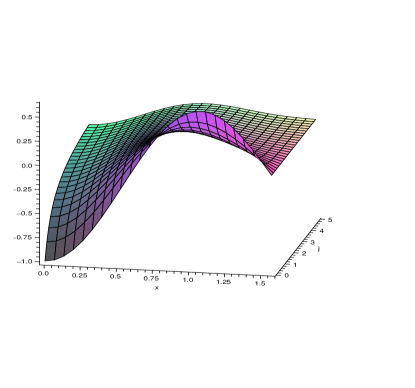
Figure 9: (Color online.) Plot of the function $X(x,j)$ with respect to $x$ and $j=J/h$. Note that there are ranges of the $(x,j)$, for which the function $X$ is positive. This fact gives rise to the phenomenon of random field induced order in the system described by the Hamiltonian $H_{h,\epsilon}$.

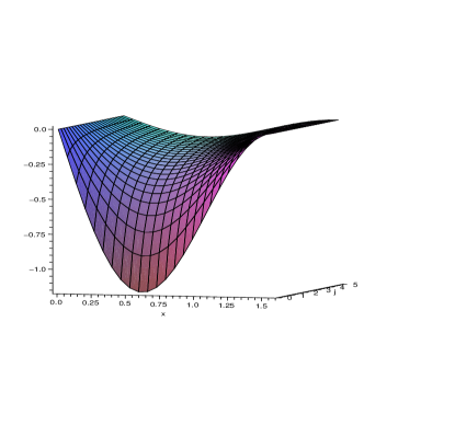
Figure 10: (Color online.) Plot of the function $Y(x,j)$ with respect to $x$ and $j$. Clearly, it is negative for the entire range of $x$ and $j$.

Therefore, at low temperatures, we have, up to order $\epsilon^{2}$:

$$m_{x}=m_{x}|_{\epsilon=0}+\epsilon^{2}\left(\frac{1}{h^{2}}X\left(x,\frac{J}{h}\right)+\mbox{order of }\frac{1}{\beta}\right),$$ (46)

$$m_{y}=m_{y}|_{\epsilon=0}+\epsilon^{2}\left(\frac{1}{h^{2}}Y\left(x,\frac{J}{h}\right)+\mbox{order of }\frac{1}{\beta}\right).$$ (47)

From Fig. 10, it is clear that the $Y$-component of the magnetization always decreases in the presence of disorder. However, Fig. 9 shows that there are ranges in the parameter space $(x,j)$, for which the quenched averaged $X$-component, $m_{x}$, of the magnetization increases in the presence of disorder, compared to the case when there is no disorder. As noted before, this is in agreement with our numerical simulations.

We have also considered the effect of disorder on the length $m$ and phase $a$ of the magnetization. For the phase, we consider the expansion of $\tan(a)=\frac{m_{y}}{m_{x}}$, which is given by

$$\tan(a)=\frac{m_{y}}{m_{x}}\Big{|}_{\epsilon=0}+\epsilon^{2}\frac{d^{2}}{d\epsilon^{2}}\left(\frac{m_{y}}{m_{x}}\right)\Big{|}_{\epsilon=0}+o(\epsilon^{2}),$$ (48)

with

$$\frac{d^{2}}{d\epsilon^{2}}\left(\frac{m_{y}}{m_{x}}\right)\Big{|}_{\epsilon=0} = \frac{m_{x}\frac{d^{2}m_{y}}{d\epsilon^{2}}-m_{y}\frac{d^{2}m_{x}}{d\epsilon^{2}}}{m_{x}^{2}}\Big{|}_{\epsilon=0}$$

$$= \frac{1}{m_{x}^{2}|_{\epsilon=0}}\frac{1}{h^{2}}S\left(x,j\right)+\mbox{order of }\frac{1}{\beta},$$

where

$$S(x,j)=Y(x,j)\cos x-X(x,j)\sin x,$$ (50)

with $X$ and $Y$ being given by Eqs. (39) and (40).

As shown in Fig. 11, $S\left(x,j\right)$ is negative for all $x$ and $j$. Consequently, the phase $a$ always bends towards the $X$-direction in the presence of disorder (since $\tan(a)$ decreases in $a$, $\cos(a)$ increases), as we have already seen in simulations. Note that $0\leq a\leq\pi/2$.

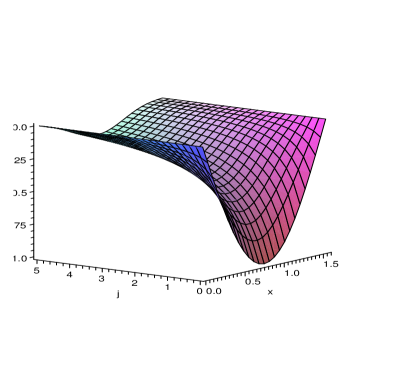
Figure 11: (Color online.) Plot of the function $S(x,j)$ with respect to $x$ and $j$. It is again negative for the entire range of $x$ and $j$. This is in agreement with the numerical results in Figs. 3 and 4.

The square of the length of the magnetization is given by (up to order $\epsilon^{2}$)

$$m_{x}^{2}+m_{y}^{2}=(m_{x}^{2}+m_{y}^{2})|_{\epsilon=0}$$

$$+2\epsilon^{2}\left((Xm_{x}+Ym_{y})|_{\epsilon=0}+\mbox{order of }\frac{1}{\beta}\right).$$ (51)

As seen on Fig. 12, $(Xm_{x}+Ym_{y})|_{\epsilon=0}$ is always negative, showing that the length of the magnetization decreases in the presence of disorder.

Figure 12: (Color online.) Plot of the function $(Xm_{x}+Ym_{y})|_{\epsilon=0}$ with respect to $x$ and $j$. It is negative for all $x$ and $j$, and numerical results in Figs. 5 and 6 corroborate this effect.

Note that the behavior of the length and phase obtained perturbatively, matches what is shown schematically in Fig. 7.

V Discussion

To summarize, we have considered classical systems of two dimensional spins, and studied the interplay between continuous symmetry and symmetry-breaking quenched disordered field, in the mean field approximation. We found that in case of a system in a uniform magnetic field, disorder may enhance one component of the order parameter.

In this paper, we have explicitly considered only the situation when the spins are two-dimensional. It is natural to ask analogous questions for three-dimensional spins with continuous symmetry. Below we argue that for the canonical system of this kind—the classical Heisenberg model—the behavior is similar to that of the XY model.

To study the behavior of magnetization in the lattice Heisenberg model in the presence of disorder, we put at all sites random fields in the Y-direction. The Hamiltonian of the resulting disordered system is given by

$$H_{H}=-J\sum_{|i-j|=1}\vec{\sigma}_{i}\cdot\vec{\sigma}_{j}-\epsilon\sum_{i}\vec{\eta}\cdot\vec{\sigma}_{i},$$ (52)

where $\vec{\eta}=\eta\cdot\vec{e}_{y}$. Here $\vec{\sigma}$ are now $3$D unit vectors. The mean field Hamiltonian is again

$$\vec{m}=-J\vec{m}\cdot\vec{\sigma}-\epsilon\vec{\eta}\cdot\vec{\sigma},$$ (53)

where $\vec{m}$ is the magnetization, and this time we parametrize $\vec{\sigma}$ as $(\sin\theta\cos\phi,\cos\theta\sin\phi,\cos\theta)$. Therefore, the mean field equation reads

$$\vec{m}=Av_{\eta}\left[\frac{\int{\vec{\sigma}}\exp(\beta J{\vec{m}}\cdot{\vec{\sigma}}+\beta\epsilon\eta\sigma_{y})\sin\theta d\theta d\phi}{\int\exp(\beta J{\vec{m}}\cdot{\vec{\sigma}}+\beta\epsilon\eta\sigma_{y})\sin\theta d\theta d\phi}\right]\equiv F_{H}(m),$$ (54)

where we have chosen

$$\vec{m}=(m\sin\psi\cos\chi,m\sin\psi\sin\chi,m\cos\psi).$$

Consider first the case, when $\epsilon=0$. By symmetry, the solutions of the mean field equation in this case form a sphere for $\beta>\beta_{c}^{0H}$.

Suppose that the radius of the sphere is $m_{0}^{H}$. To find $\beta_{c}^{0H}$ analytically, we can use an argument that is similar to the one that we have used in the case of the XY model. The existence of critical temperature gives the condition

$$F^{{}^{\prime}}_{H}(0)=\frac{\beta J}{3}>1$$ (55)

which implies

$$\beta_{c}^{0H}=\frac{3}{J}.$$

The behavior of the magnetization as $\beta$ approaches $\beta_{c}^{0H}$, is given by

$$m_{0}^{H}=\frac{\sqrt{5}}{\sqrt{2}}\frac{1}{J}(\beta_{c}^{0H})^{-\frac{3}{2}}(\beta-\beta_{c}^{0H})^{\frac{1}{2}}.$$ (56)

Note that in the case of the XY model, we also found a similar behavior of the magnetization near its critical temperature.

In the presence of disorder, i.e. $\epsilon\neq 0$, we obtain the correction to the critical temperature as

$$\beta_{c}^{\epsilon H} = \frac{3}{J}+\frac{9}{5}\frac{\epsilon^{2}}{J^{3}}+o(\epsilon^{2}),$$ (57)

$$= \beta_{c}^{0H}+\frac{9}{5}\frac{\epsilon^{2}}{J^{3}}+o(\epsilon^{2}),$$

which is again qualitatively siumilar to the situation in the XY model. The magnetization near the critical temperature is also decreased by an order of $\epsilon^{2}$. The relation between the magnetization without disorder ($m_{0}^{H}$), and that in the presence of disorder ($m^{H}$) is

$$m^{H}=m_{0}^{H}\left(1-\frac{1}{12J^{2}(m_{0}^{H})^{2}}\epsilon^{2}\right).$$ (58)

- (1) P.W. Anderson, Basic Notions of Condensed Matter Physics (Westview Press, Colorado, 1984); P.A. Lee and R.V. Ramakrishnan, Rev. Mod. Phys. 57, 287 (1985); R. Zallen, The physics of amorphous solids (Wiley, New York, 1998).
- (2) For a discussion of the recent development in the area of disordered quantum gases, see e.g. V. Ahufinger, L.Sanchez-Palencia, A. Kantian, A. Sanpera, and M. Lewenstein, Phys. Rev. A 72, 063616 (2005); M. Lewenstein, A. Sanpera, V. Ahufinger, B. Damski, A. Sen(De), and U. Sen, Adv. in Phys. 56, 243 (2007).
- (3) M. Mézard, G. Parisi, and M.A. Virasoro, Spin Glass Theory and Beyond (World Scientific, Singapore, 1987); S. Sachdev, Quantum Phase Transitions (Cambridge University Press, Cambridge, 1999); D. Chowdhury, Spin Glasses and other Frustrated Systems (Wiley, New York, 1986).
- (4) D.J. Amit, Modeling Brain Function (Cambridge University Press, Cambridge, 1989).
- (5) A. Aharony and D. Stauffer, Introduction to percolation Theory (Taylor & Francis, London, 1994); G. Grimmett, Percolation (Springer, Berlin, 1999).
- (6) A. Auerbach, Interacting electrons and Quantum magnetism (Springer, New York, 1994).
- (7) P.W. Anderson, Phys. Rev. 109, 1492 (1958); E. Abrahams, P.W. Anderson, D.C. Licciardello, and T.V. Ramakrishnan, Phys. Rev. Lett. 42, 673 (1979).
- (8) Y. Nagaoka and H. Fukuyama (Eds.), Anderson Localization, Springer Series in Solid State Sciences 39, (Springer, Heidelberg, 1982); T. Ando and H. Fukuyama (Eds.), Anderson Localization, Springer Proceedings of Physics 28, (Springer, Heidelberg, 1988).
- (9) Y. Imry and S. Ma, Phys. Rev. Lett. 35, 1399 (1975).
- (10) J.Z. Imbrie, Phys. Rev. Lett. 53, 1747 (1984); J. Bricmont and A. Kupiainen, ibid. 59, 1929 (1987).
- (11) M. Aizenman and J. Wehr, Phys. Rev. Lett. 62, 2503 (1989); M. Aizenman and J. Wehr, Comm. Math. Phys. 130, 489 (1990).
- (12) J. Wehr, A. Niederberger, L. Sanchez-Palencia, and M. Lewenstein, Phys. Rev. B 74, 224448 (2006).
- (13) C.J. Thompson, Classical equilibrium statistical mechanics (Clarendon Press, Oxford, 1988).
- (14) A. Aharony, Phys. Rev. B 18, 3328 (1978); D.E. Feldman, J. Phys. A 31, L177 (1998); B.J. Minchau and R.A. Pelcovits, Phys. Rev. B 32, 3081 (1985).
- (15) D.A. Abanin, P.A. Lee, and L.S. Levitov Phys. Rev. Lett. 98, 156801 (2007).
- (16) I.A. Fomin, J. Low Temp. Phys. 134, 97 (2005); JETP Lett. 85, 434 (2007); see also G.E. Volovik, JETP Lett. 81, 647 (2005).
- (17) A. Niederberger, T. Schulte, J. Wehr, M. Lewenstein, L. Sanchez-Palencia, and K. Sacha, arXiv:0707.0675.
- (18) D. Mermin and H. Wagner, Phys. Rev. Lett. 17, 1133 (1966); P.C. Hohenberg, Phys. Rev. 158, 383 (1967).
- (19) J. Zinn-Justin, Quantum Field Theory and Critical Phenomena, (Oxford Science Publication, Oxford, 1989).
- (20) J. Fröhlich, B. Simon, and T. Spencer, Comm. Math. Phys. 50, 79 (1976); For more general proofs, see T. Bałaban, Comm. Math. Phys. 167, 103 (1995); Comm. Math. Phys. 182, 675 (1996).
- (21) Handbook of Mathematical Functions, eds. M. Abramowitz and I.A. Stegun (Dover, New York, 1970).