Electron transport in the four-lead two-impurity Kondo model:
Nonequilibrium perturbation theory with almost degenerate levels

Abstract

The eigenstates of an isolated nanostructure may get mixed by the coupling to external leads. This effect is the stronger, the smaller the level splitting on the dot and the larger the broadening induced by the coupling to the leads is. We describe how to calculate the nondiagonal density matrix of the nanostructure efficiently in the cotunneling regime. As an example we consider a system of two quantum dots in the Kondo regime, the two spins coupled by an antiferromagnetic exchange interaction and each dot tunnel-coupled to two leads. Calculating the nonequilibrium density matrix and the corresponding current, we demonstrate the importance of the off-diagonal terms in the presence of an applied magnetic field and a finite bias-voltage.

I Introduction

In equilibrium, the occupation numbers, or more generally, the density matrix of the quantum states of an interacting electron system as a function of temperature $T$, chemical potential $\mu$ or magnetic field $B$, are given explicitly in terms of the statistical operator. Out of equilibrium, even in a stationary situation involving e.g. a current flow through the system, the statistical operator is not known in general. Statistical expectation values of observables may however be calculated for noninteracting systems, as e.g. in the Landauer formula for the conductance, or else in perturbation theory in the interaction using the method of nonequilibrium Green’s functions Rammer:86 ; Haug:96 .

A particularly simple example of the effect of a finite current on the occupation of a quantum state is the polarization of a spin-1/2 on a quantum dot in a magnetic field coupled by exchange interaction to the conduction electron spins in the leads. For sufficiently large chemical potential difference between source and drain electrodes, $\mu_{s}-\mu_{d}>g\mu_{B}B$, where $g\mu_{B}B$ is the Zeeman splitting of the local spin levels, the occupation numbers are no longer determined by the thermal Boltzmann factors, but by a rate equation. More generally, it is a quantum Boltzmann equation which describes the steady state of transitions between the two local Zeeman levels induced by the available excess energy of electrons moving from the reservoir at higher chemical potential (source) to that with lower chemical potential (drain). These processes are mediated by the exchange interaction and the resulting occupation numbers, or equivalently, the spin polarization, can be very different from their thermal equilibrium values, even in the limit of vanishing exchange coupling. For example, the spin susceptibility, which in equilibrium obeys the Curie law $\chi\propto 1/T$, is found to decrease with bias voltage $V$ as $\chi\propto 1/V$ at $T\ll eV$ (cf. Refs. Parcollet:02, ; Paaske:04, ).

In the case of a single quantum dot characterized by a spin-1/2, the density matrix of the local spin states is diagonal and the occupation numbers may be obtained, at least in lowest order in the coupling, by solving a rate equation. This is no longer the case in more complicated situations, when the density matrix is not even approximately diagonal in the basis of eigenstates of the isolated nanostructure or quantum impurity. The quantum Boltzmann equation therefore takes the form of a matrix integral-equation which can easily become numerically challenging.

We show in this paper how the quantum Boltzmann equation may be solved approximately in a controlled way with the aid of a non-unitary transformation of the matrix Green’s functions for the quantum impurity. This transformation serves to diagonalize the impurity (matrix-)spectral-function. By subsequently neglecting the broadening of these eigenstates of the cotunnel-coupled impurity, one again arrives at a simple rate-equation for the occupation numbers, valid to leading order in the cotunneling amplitude (e.g. second order in the exchange-coupling, i.e. fourth order in the tunneling amplitudes). This Bloch-Redfield Bloch:53 ; Redfield:57 ; Blum ; Slichter type equation still involves off-diagonal terms, describing the transition amplitudes for the (voltage-)driven impurity system, but it remains far simpler than the full quantum Boltzmann equation and is readily solved numerically. The Bloch-Redfield equations for the reduced density-matrix of a quantum dot have been employed in the sequential tunneling regime (cf. e.g. Refs. Engel, ; Lehmann, ). Here we demonstrate how to establish similar equations in the cotunneling, or Kondo regime, starting from the quantum Boltzmann equation.

As an example of a system where the off-diagonal entries of the density matrix become important, we study a system of two quantum dots in the Coulomb blockade regime, each accommodating a single spin-1/2, mutually coupled by a spin exchange interaction, $K$. Each dot is contacted by a set of source and drain electrodes as illustrated in Fig. 1. The eigenstates of the isolated two-impurity system are the singlet and triplet states of the two coupled spins. Nevertheless, cotunneling via the leads may mix the states, whereby the density matrix of the two-impurity system will acquire off-diagonal terms. As demonstrated below, this mixing can only occur in the presence of an applied magnetic field and for asymmetric couplings to the leads. The simpler case of zero magnetic field has already been analyzed in a previous publication Koerting:07 . For $K=0$, the product states of the two spin-1/2 would be a natural basis, but for any finite $K$, perturbation theory should be performed with respect to the singlet/triplet basis. We will demonstrate how the singlet/triplet basis can be used, even for $K=0$, as long as the off-diagonal parts of the density matrix are properly taken into account.

II Four-lead Two-impurity Kondo model

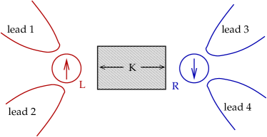
Figure 1: (color online) Double quantum dot setup: Two Kondo impurities, $L,R$, both represented by a spin-1/2 are coupled mutually by a spin exchange interaction $K$. The quantum dots are connected to two leads each, $1,2$ and $3,4$, respectively.

We model this four-lead two-impurity Kondo model as illustrated in Fig. 1 by the Hamiltonian

$$H =\sum_{\mathbf{k}n\sigma}(\epsilon_{k}-\mu_{n})c_{n\mathbf{k}\sigma}^{\dagger}c_{n\mathbf{k}\sigma}$$ (1)

$$+K\mathbf{S}_{L}\cdot\mathbf{S}_{R}-g\mu_{B}\mathbf{B}\cdot(\mathbf{S}_{L}+\mathbf{S}_{R})$$

$$+{\textstyle\sum\limits_{n,m=1,2}}J_{L}^{nm}\,\mathbf{S}_{L}\cdot\mathbf{s}_{nm}+{\textstyle\sum\limits_{n,m=3,4}}J_{R}^{nm}\,\mathbf{S}_{R}\cdot\mathbf{s}_{nm},$$

where $n,m=1,2,3,4$ labels the leads, which are characterized by the same constant density of states near the Fermi level, $N(0)$, but with generally different chemical potentials $\mu_{n}$. The spin-operator $\mathbf{s}_{nm}=\sum_{\mathbf{k},\mathbf{k}^{\prime},\sigma,\sigma^{\prime}}c_{n\mathbf{k}\sigma}^{\dagger}(\vec{\tau}_{\sigma,\sigma\prime}/2)c_{m\mathbf{k}^{\prime}\sigma^{\prime}}$ denotes respectively the conduction electron spin ($n=m$) and the exchange tunneling operator ($n\neq m$). Notice that we do not allow for charge transfer between the two dots. As we have demonstrated earlier Koerting:07 , the coupling to two pairs of source, and drain electrodes gives rise to a marked transconductance signal, reflecting the onset of cotunneling current through the left dot, say, when tuning the voltage over the right dot to match the exchange coupling, i.e. $\mu_{3}-\mu_{4}=K$.

The eigenstates of the isolated two-impurity spin system are the singlet and triplet states

$$|t_{+}\rangle =|\uparrow\rangle_{L}|\uparrow\rangle_{R},$$

$$|t_{0}\rangle =\frac{1}{\sqrt{2}}\left(|\uparrow\rangle_{L}|\downarrow\rangle_{R}+|\downarrow\rangle_{L}|\uparrow\rangle_{R}\right),$$

$$|t_{-}\rangle =|\downarrow\rangle_{L}|\downarrow\rangle_{R},$$

$$|s\rangle =\frac{1}{\sqrt{2}}\left(|\uparrow\rangle_{L}|\downarrow\rangle_{R}-|\downarrow\rangle_{L}|\uparrow\rangle_{R}\right).$$

For $K=0$, however, it would be more reasonable to use the product states

$$|1\rangle =|\uparrow\rangle_{L}|\downarrow\rangle_{R},\qquad|2\rangle=|\downarrow\rangle_{L}|\uparrow\rangle_{R},$$

$$|3\rangle =|\uparrow\rangle_{L}|\uparrow\rangle_{R},\qquad|4\rangle=|\downarrow\rangle_{L}|\downarrow\rangle_{R},$$

of the left and the right spin as a basis. Expressing the latter basis in terms of the former, the eigenstates with total spin quantum number $S_{z}=0$ are seen to mix:

$$|1\rangle =|\uparrow\rangle_{L}|\downarrow\rangle_{R}=\frac{1}{\sqrt{2}}\left(|t_{0}\rangle+|s\rangle\right),$$

$$|2\rangle =|\downarrow\rangle_{L}|\uparrow\rangle_{R}=\frac{1}{\sqrt{2}}\left(|t_{0}\rangle-|s\rangle\right),$$ (2)

$$|3\rangle =|t_{+}\rangle,\quad|4\rangle=|t_{-}\rangle.$$

In order to have a convenient representation of the spin operators in the singlet-triplet basis, we define a set of pseudo-boson (pb) operators $\{b_{\gamma}^{\dagger}\}=\{s^{\dagger},t_{+}^{\dagger},t_{0}^{\dagger},t_{-}^{\dagger}\}$, i.e. $\gamma\in\{s,t_{+},t_{0},t_{-}\}$, to describe creation(annihilation) of a singlet state $s^{{\dagger}}$($s$) or a triplet state $t_{\gamma}^{{\dagger}}$($t_{\gamma}$) Sachdev:90 . The operators $b_{\gamma}^{\dagger}$ span an infinite dimensional Fock space, which has to be projected onto the physical Hilbert space, in which only single occupancy is allowed, i.e. $Q=s^{\dagger}s+t_{0}^{\dagger}t_{0}+t_{+}^{\dagger}t_{+}+t_{-}^{\dagger}t_{-}=1$. This constraint is enforced by adding a term $\lambda Q$ to the Hamiltonian and taking the limit $\lambda\rightarrow\infty$ Abrikosov:65 when calculating physical observables. The energy eigenvalues of the four states are

$$\omega_{s}=-\frac{3}{4}K,\quad\omega_{t_{0}}=\frac{1}{4}K,\quad\omega_{t_{\pm}}=\frac{1}{4}K\mp B,$$

and therefore

$$K\ \mathbf{S}_{L}\cdot\mathbf{S}_{R}=\omega_{s}s^{{\dagger}}s+\sum_{\gamma}\omega_{t_{0}}t_{\gamma}^{\dagger}t_{\gamma}.$$

In terms of the pseudo bosons, the spin-1/2 operators at the left/right dot are given by

$$S_{L/R}^{z} =\frac{1}{2}(\pm s^{\dagger}t_{0}\pm t_{0}^{\dagger}s+t_{+}^{\dagger}t_{+}-t_{-}^{\dagger}t_{-}),$$ (3)

$$S_{L/R}^{+}=(S_{L/R}^{-})^{\dagger} =\frac{1}{2}(\pm s^{\dagger}t_{-}\mp t_{+}^{\dagger}s+t_{+}^{\dagger}t_{0}+t_{0}^{\dagger}t_{-}).$$ (4)

Or in compact notation, with $\alpha=L,R$,

$$\mathbf{S}_{\alpha}=\frac{1}{2}\sum_{\gamma,\gamma^{\prime}}\ b_{\gamma}^{\dagger}\mathbf{T}_{\alpha;\gamma\gamma^{\prime}}b_{\gamma^{\prime}},$$

where $\mathbf{T}_{\alpha;\gamma\gamma^{\prime}}$ is a vector of three 4x4 matrices, $T^{x},T^{y},T^{z}$, defined by

$$T_{L/R}^{z}=\begin{pmatrix}0&0&\pm 1&0\\ 0&1&0&0\\ \pm 1&0&0&0\\ 0&0&0&-1\end{pmatrix},\quad T_{L/R}^{+}=\begin{pmatrix}0&0&0&\pm 1\\ \mp 1&0&1&0\\ 0&0&0&1\\ 0&0&0&0\end{pmatrix},$$

where $T_{\alpha}^{+}=(T_{\alpha}^{-})^{{\dagger}}=\frac{1}{\sqrt{2}}(T_{\alpha}^{x}+iT_{\alpha}^{y})$.

It is worth noting that the representation of $\mathbf{S}_{L/R}$, Eqs. (3) and (4), does not include an $s^{{\dagger}}s$ term, but only transition operators from a singlet to a triplet state. This implies, for example, that exchange-tunneling current cannot pass through either of the two quantum dots if the two-impurity system is in the singlet state. Interestingly, the excitation gap, $K$, to the current-carrying triplet states can be overcome by a finite bias across either of the two dots. This gives rise to a pronounced transconductance signal, which we have investigated earlier in Ref. Koerting:07, . This work was restricted to zero magnetic field and hence avoided the problem of off-diagonal terms in the nonequilibrium correlation functions.

III Density matrix and occupation numbers

Assuming the exchange-tunneling to be weak, i.e. $N(0)J_{\alpha}^{nm}\ll 1$, we shall determine the singlet-triplet occupation numbers by means of nonequilibrium perturbation theory. We employ contour-ordered Green’s functions arranged in the matrix-form

$$\mathbf{G}=\begin{pmatrix}G^{<}+G^{r}&G^{>}\\ G^{<}&G^{>}-G^{r}\end{pmatrix},$$

satisfying the Dyson equation

$$\mathbf{G}_{0}^{-1}\mathbf{G}=\mathbf{1}+\mathbf{\Sigma G},$$

where $\mathbf{G}$ and $\mathbf{G}_{0}$ are the dressed and bare contour-ordered matrix Green’s functions and $\mathbf{\Sigma}$ is the self energy.

Whereas the information on the energy spectrum, including any shifts by external fields, is encoded in the retarded Green’s function $G^{r}$, the information on the thermodynamic state of the system, i.e. the occupation of the energy levels, is contained in $G^{<}.$ Out of equilibrium, these two functions are not simply connected through a fluctuation-dissipation theorem and instead one must solve one more component of the matrix Dyson equation,

$$G_{0}^{-1}\,G^{<}=\Sigma^{r}G^{<}+\Sigma^{<}G^{a}.$$

An equivalent equation is obtained by applying $\mathbf{G}_{0}^{-1}$ to the second time argument in $\mathbf{G}$ (cf. Ref. Haug:96, ). In contrast to the Dyson equation for $G^{r},$ this quantum Boltzmann equation is a self-consistent equation for $G^{<}$, since $\Sigma^{<}$ also depends on $G^{<}$ and since no unrenormalized $G^{<}_{0}$ is known for an isolated quantum impurity. In the limit of vanishing coupling to the leads, $G^{<}$ is found to be independent of that coupling. Therefore the occupation number

$$n=i\int\frac{d\omega}{2\pi}\,G^{<}(\omega)$$

can take a finite limiting value dependent on the system parameters temperature, bias voltage and magnetic field in $0$th order in the coupling to the leads (cf. also Refs. Parcollet:02, ; Paaske:04, ).

In the example of a two-impurity system, the pb Green’s functions form a matrix in the singlet-triplet (ST) basis $\gamma=\{s,t_{+},t_{0},t_{-}\}$, i.e.

$$\mathcal{G}^{r}=\begin{pmatrix}G_{ss}^{r}&0&G_{st_{0}}^{r}&0\\ 0&G_{t_{+}t_{+}}^{r}&0&0\\ G_{t_{0}s}^{r}&0&G_{t_{0}t_{0}}^{r}&0\\ 0&0&0&G_{t_{-}t_{-}}^{r}\end{pmatrix},$$

where only the elements allowed by symmetry are shown.

Notice that in the absence of any coupling to the leads, but assuming coupling to a heat bath, the quantum impurity is in thermodynamic equilibrium and the Green’s functions are given immediately as

$$G_{\gamma\gamma}^{<,(0)}(\omega) =-in_{B}(\omega)A_{\gamma\gamma}^{(0)}(\omega),$$ (5)

$$G_{\gamma\gamma}^{>,(0)}(\omega) =-i[n_{B}(\omega)+1]A_{\gamma\gamma}^{(0)}(\omega),$$ (6)

$$G_{\gamma\gamma}^{r/a,(0)}(\omega) =\frac{1}{\omega-\omega_{\gamma}-\lambda\pm i\delta},$$ (7)

$$A_{\gamma\gamma}^{(0)}(\omega) =2\pi\delta(\omega-\omega_{\gamma}-\lambda),$$ (8)

where $\omega_{\gamma}$ is the energy of the state $\gamma\in\{s,t_{+},t_{0},t_{-}\}$ and $n_{B}(\omega)$ is the Bose distribution function. In the limit $\lambda\rightarrow\infty$ the Bose function at the position of the spectral peak, $\omega=\omega_{\gamma}+\lambda,$ turns into a Boltzmann factor $n_{\gamma}\varpropto e^{-\beta(\omega_{\gamma}+\lambda)}\ll 1$. The difference between the Bose and the Fermi statistics for the pseudo particles is then seen to vanish. Any term containing a product of two occupation numbers $n_{\gamma}^{\lambda}n_{\gamma^{\prime}}^{\lambda}\propto e^{-2\beta\lambda}$ will be projected out at the end of the calculation.

III.1 Pseudo-boson self energy

The first order (in $N(0)J_{\alpha}^{nm}$) pseudo-boson self energy is proportional to the spin polarization of the conduction electrons. It provides only a correction to the g-factor of the local spin and will be neglected in the following.

\psfrag{b}{$\beta,\beta^{\prime}$}\psfrag{g}{$\gamma$}\psfrag{g'}{$\gamma^{\prime}$}\includegraphics{selfenerg.eps}

Figure 2: Diagram for the second order pseudo boson self energy. Solid lines: conduction electron Green’s functions, dashed lines: pseudo particles of the double quantum dot system.

The second order self energy, on the other hand, corresponds to the diagram in Fig. 2 and reads

$$\Sigma_{\gamma^{\prime}\gamma}(\tau_{1},\tau_{2})=-\frac{1}{16} \sum\limits_{\alpha=L,R}Y_{\alpha}(\tau_{1},\tau_{2})$$ (9)

$$\times\sum_{\beta,\beta\prime}\mathbf{T}_{\alpha;\gamma^{\prime}\beta}\ G_{\beta,\beta^{\prime}}(\tau_{1},\tau_{2})\mathbf{T}_{\alpha;\beta^{\prime}\gamma}.$$

Here the time variables $\tau_{1,}\tau_{2}$ lie on the Schwinger contour, and $\alpha=L(R)$ for $m,n=1,2,(3,4)$. We have introduced the abbreviation,

$$Y_{\alpha}(\tau_{1},\tau_{2})=2\!\!\!\!\!\!\sum_{m,n=1,2,(3,4)}J_{\alpha}^{mn}J_{\alpha}^{nm}\,X_{n}^{m}(\tau_{1},\tau_{2}),$$ (10)

with the summation variables depending on $\alpha$ and with

$$X_{m}^{n}(\tau_{1},\tau_{2})=\frac{1}{(-i)^{2}}\sum_{k,k^{\prime}}G_{nk^{\prime}}(\tau_{2},\tau_{1})G_{mk}(\tau_{1},\tau_{2})$$

being the conduction electron susceptibility.

This expression is quite general and would be valid for any quantum impurity with internal states $\gamma$, where the matrices $\mathbf{T}_{\alpha}^{i}$ would have to be defined accordingly. The self energy will have off-diagonal components $(\gamma\neq\gamma\prime)$ if the conservation laws for spin allow so. Since a conduction electron tunneling through one of the dots can either flip its spin or not, the accessible intermediate states may change the quantum number $S_{z}$ by $0,\pm 1$. The second process has to flip the conduction electron spin back. Therefore, the self energy is diagonal in the quantum number $S_{z}$. For the double dot considered here this leaves only one possible off-diagonal element, $st_{0}$ (and its hermitian conjugate), given by

$$\Sigma_{st_{0}}(\tau_{1},\tau_{2})=-\frac{1}{16} \left(G_{t_{0}s}(\tau_{1},\tau_{2})[Y_{L}(\tau_{1},\tau_{2})+Y_{R}(\tau_{1},\tau_{2})]\right.$$

$$+[G_{t_{-}t_{-}}(\tau_{1},\tau_{2})-G_{t_{+}t_{+}}(\tau_{1},\tau_{2})]$$

$$\left.\hskip 8.53581pt\times[Y_{L}(\tau_{1},\tau_{2})-Y_{R}(\tau_{1},\tau_{2})]\right).$$ (11)

All other elements of the self energy are given in appendix A. We emphasize that the off-diagonal self energy is finite only if two symmetries are broken simultaneously: time reversal symmetry by a magnetic field $(t_{+}\not=t_{-})$ and parity, i.e. the left-right symmetry $(Y_{L}\not=Y_{R})$.

\psfrag{t0}{\footnotesize$t_{0}$}\psfrag{t+}{\footnotesize$t_{+}$}\psfrag{t-}{\footnotesize$t_{-}$}\includegraphics[width=173.44534pt]{explain_st0_imp.eps}

Figure 3: (color online) Illustration of the symmetry in the off-diagonal self energy $\Sigma_{st_{0}}$. The two different paths from the singlet-state $|s\rangle$ to the triplet-state $|t_{0}\rangle$ over $|t_{-}\rangle$ and $|t_{+}\rangle$ come with opposite signs. Green(left) sign for interaction with left leads. Red(right) sign for interaction with right leads.

This can be understood from the following simple argument. Starting from the singlet state, a flipping of the left spin, say, causes a transition to a triplet state with $S_{tot}^{z}\not=0$,

$$S_{L}^{\mp}|s\rangle=\pm\frac{1}{\sqrt{2}}|t_{\mp}\rangle,$$ (12)

which, upon a subsequent flipping of the left spin, makes a transition to either $|s\rangle$ or $|t_{0}\rangle$. This is illustrated in Fig. 3. The two intermediate triplet states come with opposite signs, i.e. shifted in phase by $\pi$, and in the case of zero magnetic field these two alternative paths from $|s\rangle$ to $|t_{0}\rangle$ cancel and $\Sigma_{st_{0}}$ vanishes. This is not the case for the diagonal component $\Sigma_{ss}$ in which the signs are squared and cause no cancellation. The observed dependence on the left-right symmetry, indicated in Fig. 3, arises in a similar way.

Performing the analytical continuation to the real-time axis, one finds after Fourier-transformation in the relative time-variable,

$$Y_{L}^{<}(\omega)= (-2\pi)\left[\left(g_{11}^{2}+g_{22}^{2}\right)2B(\omega)\right.$$ (13)

$$\left.+2g_{12}g_{21}\left(B(\omega+eV_{L})+B(\omega-eV_{L})\right)\right],$$

$$Y_{R}^{<}(\omega)= (-2\pi)\left[\left(g_{33}^{2}+g_{44}^{2}\right)2\,B(\omega)\right.$$ (14)

$$\left.+2g_{34}g_{43}\left(B(\omega+eV_{R})+B(\omega-eV_{R})\right)\right],$$

and $g_{nm}=N(0)J^{nm},Y_{L\pm R}^{<}(\omega)=Y_{L}^{<}(\omega)\pm Y_{R}^{<}(\omega)$, where we have introduced the function

$$B(x)=x\cdot n_{B}(x)=\left[\coth(\beta x/2)-1\right]x/2.$$

From these correlation functions, the lesser component and the imaginary part of the retarded self energy are obtained as

$$\Sigma_{st_{0}}^{<}(\omega) =-\frac{1}{16}\int\frac{d\epsilon}{2\pi}\,\left\{G_{t_{0}s}^{<}(\epsilon)Y_{L+R}^{<}(\omega-\epsilon)\right.$$

$$\qquad\qquad+\left.\left(G_{t_{-}t_{-}}^{<}(\epsilon)-G_{t_{+}t_{+}}^{<}(\epsilon)\right)Y_{L-R}^{<}(\omega-\epsilon)\right\},$$ (15)

$$\Gamma_{st_{0}}(\omega) =2i\mathrm{Im}\Sigma_{st_{0}}^{r}\approx-2\frac{1}{16}\int\frac{d\epsilon}{2\pi}\{\,A_{t_{0}s}(\epsilon)Y_{L+R}^{<}(\epsilon-\omega)$$

$$\qquad\qquad+\left(A_{t_{-}t_{-}}(\epsilon)-A_{t_{+}t_{+}}(\epsilon)\right)Y_{L-R}^{<}(\epsilon-\omega)\}.$$ (16)

We observe that the off-diagonal spectral function obeys the sum rule

$$\int\frac{d\omega}{2\pi}A_{st_{0}}(\omega)=\left\langle[s,t_{0}^{{\dagger}}]\right\rangle=0.$$

From the hermiticity condition it follows that

$$\left[G_{st_{0}}^{r}(\omega)\right]^{\ast}=G_{t_{0}s}^{a}(\omega),$$ (17)

and thus the spectral functions,

$$A_{st_{0}}(\omega)=A_{t_{0}s}(\omega),$$

are identical. In addition one has

$$\left[G_{st_{0}}^{<}(t)\right]^{\ast}=-G_{t_{0}s}^{<}(-t)$$

$$\Rightarrow\qquad \left\{\begin{matrix}\mathrm{Re}\left[G_{st_{0}}^{<}(\omega)\right]=-\mathrm{Re}\left[G_{t_{0}s}^{<}(\omega)\right]\\ \mathrm{Im}\left[G_{st_{0}}^{<}(\omega)\right]=\mathrm{Im}\left[G_{t_{0}s}^{<}(\omega)\right]\end{matrix}\right.$$ (18)

The diagonal elements of $G_{\gamma\gamma\prime}^{<}$ are purely imaginary functions, and the off-diagonal elements share this property approximately

$$\mathrm{Re}\left[G_{st_{0}}^{<}(\omega)\right] =-\mathrm{Re}\left[G_{t_{0}s}^{<}(\omega)\right]\approx 0$$

$$\Rightarrow G_{st_{0}}^{<}(\omega) \approx G_{t_{0}s}^{<}(\omega)$$ (19)

Thus the lesser Green’s function is assumed to be symmetric in analogy to the spectral function which was proven to be symmetric. It follows straightforwardly that $\Sigma_{st_{0}}=\Sigma_{t_{0}s}$.

III.2 Retarded Green’s function

Assuming that the off-diagonal self energy is finite, we find by solving Dyson’s equation $\mathcal{G}^{r}=[(\mathcal{G}^{r,(0)})^{-1}-\Sigma^{r}]^{-1}$,

$$\mathcal{G}^{r}=\frac{1}{\mathrm{det}}\begin{pmatrix}(G_{t_{0}t_{0}}^{r})^{-1}&0&\Sigma_{st_{0}}^{r}&0\\ 0&\mathrm{det}\cdot G_{t_{+}t_{+}}^{r}&0&0\\ \Sigma_{st_{0}}^{r}&0&(G_{ss}^{r})^{-1}&0\\ 0&0&0&\mathrm{det}\cdot G_{t_{-}t_{-}}^{r}\end{pmatrix},$$

where $(G_{\gamma\gamma}^{r})^{-1}=\omega-\omega_{\gamma}-\Sigma_{\gamma\gamma}^{r}$ and $\mathrm{det}=(G_{t_{0}t_{0}}^{r})^{-1}(G_{ss}^{r})^{-1}-(\Sigma_{st_{0}}^{r})^{2}$.

To lowest order in the coupling to the leads the retarded self energy is of $\mathcal{O}(g^{2})$, and the off-diagonal Green’s function is given by $\Sigma_{st_{0}}^{r}/\mathrm{det}$. Since the total spectral weight of the off-diagonal spectral function vanishes, the function changes sign. It can be shown that it is approximately given by the difference of two Lorentzians, see illustration in Fig. 4. Since $A_{st_{0}}(\epsilon)$ is not characterized by a single peak, integration over $\epsilon$ of a product of $A_{st_{0}}(\epsilon)$ and a more slowly varying function $B(\epsilon)$ may not be approximated as usual by taking $B(\epsilon)$ at the position of the peak.

\psfrag{Ass}{$A_{ss}(\omega)$}\psfrag{Ast0}{$A_{st_{0}}(\omega)$}\psfrag{At0t0}{$A_{t_{0}t_{0}}(\omega)$}\psfrag{w/B}{$\omega/B$}\includegraphics*[width=195.12767pt]{Asto_new.eps}

Figure 4: (color online) Spectral functions $A_{ss},A_{st_{0}}$ and $A_{t_{0}t_{0}}$ versus the frequency $\omega/B$ for an exchange spin interaction $K$ of the order of the level broadening, $K=0.05\sim\Gamma_{st_{0}}$. Further parameters are $B=1.0$, $g_{L}=0.1$, $g_{R}=0.2$ and $T=0.001$. The off-diagonal spectral function $A_{st_{0}}$ has total spectral weight zero and thus contains negative values.

In order to avoid having to deal with a not positive definite spectral function we may diagonalize the retarded Green’s function matrix. The transformed matrix is given by

$$(U^{r})_{\gamma_{1}\gamma}^{-1}\mathcal{G}_{\gamma\gamma^{\prime}}^{r}U_{\gamma^{\prime}\gamma_{2}}^{r} =\tilde{\mathcal{G}}_{\gamma_{1}\gamma_{2}}^{r},$$

$$\mathrm{and}\qquad\tilde{\mathcal{G}}_{\gamma_{1}\gamma_{2}}^{r} =\begin{pmatrix}G_{11}^{r}&0&0&0\\ 0&G_{t_{+}t_{+}}^{r}&0&0\\ 0&0&G_{22}^{r}&0\\ 0&0&0&G_{t_{-}t_{-}}^{r}\\ \end{pmatrix},$$

where $G_{11}^{r}=1/(\omega-\omega_{1}^{r})$ and $G_{22}^{r}=1/(\omega-\omega_{2}^{r})$ with

$$\omega_{1/2}^{r}= -\frac{1}{2}\left(\omega_{t_{0}}+\Sigma^{r}_{t_{0}t_{0}}(\omega)+\omega_{s}+\Sigma^{r}_{ss}(\omega)\right)$$

$$\pm\frac{1}{2}\sqrt{\left(\omega_{t_{0}}+\Sigma^{r}_{t_{0}t_{0}}(\omega)-\omega_{s}-\Sigma_{ss}^{r}(\omega)\right)^{2}+4\,\left(\Sigma_{st_{0}}^{r}\right)^{2}}.$$

This rotation is important only in the case when $\Sigma_{st_{0}}^{r}$ becomes of the same order of magnitude as the first term in the square root, which is proportional to the singlet-triplet splitting $\omega_{t_{0}}-\omega_{s}=K$. The transformation matrix is given by

$$U^{r}=\begin{pmatrix}x_{1}^{r}&0&-x_{2}^{r}&0\\ 0&1&0&0\\ x_{2}^{r}&0&x_{1}^{r}&0\\ 0&0&0&1\end{pmatrix}$$

with the already normalized value of $x_{1}^{r}=(x^{\prime})_{1}^{r}/\mathcal{N}^{r}$ and $x_{2}^{r}=(x^{\prime})_{2}^{r}/\mathcal{N}^{r}$ where $\mathcal{N}^{r}=\sqrt{\left((x^{\prime})_{1}^{r}\right)^{2}+\left((x^{\prime})_{2}^{r}\right)^{2}}$ and

$$(x^{\prime})_{1}^{r}= \frac{1}{2}\left((G_{ss}^{r}(\omega))^{-1}-(G_{t_{0}t_{0}}^{r}(\omega))^{-1}\right)$$

$$+\frac{1}{2}\sqrt{\left((G_{ss}^{r}(\omega))^{-1}-(G_{t_{0}t_{0}}^{r}(\omega))^{-1}\right)^{2}+4\,\left(\Sigma_{st_{0}}^{r}\right)^{2}},$$

$$(x^{\prime})_{2}^{r}= -\Sigma_{st_{0}}^{r}.$$

The transformation matrix $U^{r}$ has complex valued elements and its inverse is equal to its transpose. For $K=0$, we find $x_{1}^{r}=-x_{2}^{r}=1/\sqrt{2}$ and the eigenstates of the system are given by the product states of the double quantum dot system, $|1\rangle=\frac{1}{\sqrt{2}}(|t_{0}\rangle+|s\rangle)$ and $|2\rangle=\frac{1}{\sqrt{2}}(|t_{0}\rangle-|s\rangle)$.

The transformation of the advanced Green’s function is different,

$$\left(U^{a}\right)^{-1}\mathcal{G}^{a}U^{a}=\tilde{\mathcal{G}}^{a},$$

where the transformation matrix $U^{a}$ is defined in analogy to the retarded Green’s function with $r$ replaced by $a$. The transformation matrix $U^{a}$ is related to $U^{r}$ by $\left[U^{a}\right]^{\dagger}=\left[U^{r}\right]^{-1}$, so that $[\tilde{\mathcal{G}}^{r}]^{\dagger}=\tilde{\mathcal{G}}^{a}$. Since $\widetilde{G}_{11}^{r},\widetilde{G}_{22}^{r}$ are characterized by a single pole, the corresponding spectral functions show a single sharp peak and the commutation relations of the boson operators guarantee the integrated weight unity.

\psfrag{A11}{$\widetilde{A}_{11}(\omega)$}\psfrag{A22}{$\widetilde{A}_{22}(\omega)$}\psfrag{w/B}{$\omega/B$}\includegraphics*[width=195.12767pt]{A11_A22_new.eps}

Figure 5: (color online) Spectral functions $\widetilde{A}_{11}(\omega)$ and $\widetilde{A}_{22}(\omega)$ versus the frequency $\omega/B$ in the rotated space for the same parameter set as in Fig. 4.

In Fig. 5 we show a typical example of the spectral functions $\widetilde{A}_{ii}(\omega)=-2\operatorname{Im}$ $\widetilde{G}_{ii}^{r}$, $i=1,2$ .

III.3 Lesser Green’s function

As mentioned above, the lesser Green’s function has to be calculated self-consistently, e.g. in lowest order perturbation theory, thus in this model to second order.

The lesser components of the Dyson equation are given by one of the equations

$$\left(\mathcal{G}^{r}\right)^{-1}\,\mathcal{G}^{<} =\Sigma^{<}\,\mathcal{G}^{a},$$

$$\mathcal{G}^{<}\left(\mathcal{G}^{a}\right)^{-1} =\mathcal{G}^{r}\,\Sigma^{<},$$

where we neglected the boundary terms. Subtracting these two equations, $G^{<}$ is found to obey the quantum Boltzmann equation Haug:96 ,

$$\left(\mathcal{G}^{r}\right)^{-1}\,\mathcal{G}^{<}-\mathcal{G}^{<}\,\left(\mathcal{G}^{a}\right)^{-1}=\Sigma^{<}\,\mathcal{G}^{a}-\mathcal{G}^{r}\,\Sigma^{<}.$$ (20)

If we neglect the off-diagonal terms in Eq. (20) we have to solve the following equations,

$$\left[\left(G^{r}\right)^{-1}-\left(G^{a}\right)^{-1}\right]_{\gamma\gamma}\,G_{\gamma\gamma}^{<} =\Sigma_{\gamma\gamma}^{<}\,\left[G^{a}-G^{r}\right]_{\gamma\gamma}$$

$$\Rightarrow\quad G_{\gamma\gamma}^{<}(\omega) =\frac{\Sigma_{\gamma\gamma}^{<}(\omega)}{\Gamma_{\gamma\gamma}(\omega)}\,A_{\gamma\gamma}(\omega),$$

which is a self-consistency equation for the occupation number $n_{\gamma}=i\,\Sigma_{\gamma\gamma}^{<}(\omega_{\gamma})/\Gamma_{\gamma\gamma}(\omega_{\gamma})$. Since the broadening of the spectral function $A_{\gamma\gamma}$ is the smallest energy scale in the problem, we neglect the frequency dependence and consider only the on-shell occupation numbers. In this lowest order approximation the quantum Boltzmann equation (20) is essentially a rate equation (see appendix B for explicit expressions of the occupation numbers), albeit one which now includes the off-diagonal components of the density matrix.

We will now demonstrate how this approach fails in the example of the magnetization. For $K=0$, the left and the right spins as defined in Eq. (3) are good quantum numbers and we can define the corresponding magnetizations

$$M_{L/R}=2\langle S_{L/R}^{z}\rangle=\left\langle t_{+}^{{\dagger}}t_{+}-t_{-}^{{\dagger}}t_{-}\right\rangle$$

under the assumption that $\langle s^{{\dagger}}t_{0}+t_{0}^{{\dagger}}s\rangle=0$. This leads to

$$M_{L/R}=\frac{Y_{L}^{<}(B)+Y_{R}^{<}(B)-Y_{L}^{<}(-B)-Y_{R}^{<}(-B)}{Y_{L}^{<}(B)+Y_{R}^{<}(B)+Y_{L}^{<}(-B)+Y_{R}^{<}(-B)},$$

from which the magnetization on the left quantum dot is found to depend on the magnetization of the right quantum dot and vice versa, even though the dots are completely decoupled. For a single Kondo impurity, however, the correct result is Parcollet:02 ; Paaske:04

$$M_{L}=\frac{Y_{L}^{<}(B)-Y^{<}_{L}(-B)}{Y^{<}_{L}(B)+Y^{<}_{L}(-B)}.$$ (21)

The off-diagonal components are not important in the case of left-right symmetry and indeed for $Y_{L}=Y_{R}$ we obtain the correct expression for $M_{L}$. Also, at $B=0$ and consequently $M_{L}=0$ the two different results coincide. The difference of the two above results for $M_{L}$ can be traced back to the unjustified neglect of the off-diagonal average $\langle s^{{\dagger}}t_{0}+t_{0}^{{\dagger}}s\rangle$. We show in the appendix C that including the effect of off-diagonal terms, by employing the transformation defined above, we recover the correct result for the magnetization $M_{L}$, Eq. (21). From this calculation it is obvious that the off-diagonal terms contribute to the same order as the diagonal terms.

In the case of finite exchange interaction $K$ the calculation including the off-diagonal contributions becomes cumbersome, since one has to solve a self-consistent system of integral equations. The solution can be much simplified in the transformed basis introduced above.

To rotate the Quantum Boltzmann equation we multiply Eq. (20) with $U^{r}$ from the left and $(U^{a})^{-1}=(U^{r})^{\dagger}$ from the right. Thus we find the transformed quantum Boltzmann equation,

$$(\tilde{\mathcal{G}}^{r})^{-1}\,\tilde{\mathcal{G}}^{<}-\tilde{\mathcal{G}}^{<}\,(\tilde{\mathcal{G}}^{a})^{-1}=\tilde{\Sigma}^{<}\,\tilde{\mathcal{G}}^{a}-\tilde{\mathcal{G}}^{r}\,\tilde{\Sigma}^{<}$$ (22)

where $\tilde{\Sigma}^{<}=U^{r}\Sigma^{<}(U^{a})^{-1}=U^{r}\Sigma^{<}(U^{r})^{\dagger}$ and $\tilde{\mathcal{G}}^{<}=U^{r}\mathcal{G}^{<}(U^{a})^{-1}=U^{r}\mathcal{G}^{<}(U^{r})^{\dagger}$. After the transformation all retarded and advanced Green’s functions are diagonal and we obtain a single equation for every entry of the lesser Green’s function. There is still a finite off-diagonal element $\tilde{G}_{(1,2)}^{<}$ in the rotated basis, and the big advantage over the initial formulation is the fact that the spectral functions appearing on the r.h.s. of Eq. (22) are now all positive definite and may be approximated by delta functions of weight unity. As for the corresponding real parts of $\tilde{\mathcal{G}}^{a,r}$ we adopt the usual assumption that after frequency integration they may be neglected. From Eq. (22) $\tilde{\mathcal{G}}^{<}$ is then found as a sum of delta functions with weights $\widetilde{\emph{N}}^{\gamma}$ to be determined self-consistently,

$$\,\tilde{\mathcal{G}}^{<}=-i{\textstyle\sum\limits_{\gamma=1,2,t_{+},t_{-}}}\widetilde{\emph{N}}^{\gamma}2\pi\delta(\omega-\omega_{\gamma}).$$

This expression, when substituted into the lesser self energy, leads to a linear combination of weight factors. The quantum Boltzmann equation reduces to a set of linear homogeneous equations for $\widetilde{\emph{N}}^{\gamma}$, which, together with the normalization condition, $s^{\dagger}s+t_{0}^{\dagger}t_{0}+t_{+}^{\dagger}t_{+}+t_{-}^{\dagger}t_{-}=1$, may be solved to give the weight factors. Note that $\widetilde{\emph{N}}^{\gamma}$ are matrices in the local Hilbert space defined by states $(1,t_{+},2,t_{-})$ with nonzero components $\widetilde{N}_{t_{+}t_{+}}^{\gamma}$, $\widetilde{N}_{t_{-}t_{-}}^{\gamma}$, $\widetilde{N}_{11}^{\gamma}$, $\widetilde{N}_{22}^{\gamma}$, $\widetilde{N}_{12}^{\gamma}$ and $\widetilde{N}_{21}^{\gamma}$.

The expectation value $\langle s^{{\dagger}}t_{0}+t_{0}^{{\dagger}}s\rangle$ is obtained from $G_{st_{0}}^{<}$ as

$$\langle s^{{\dagger}}t_{0}+t_{0}^{{\dagger}}s\rangle =i\int\frac{d\omega}{2\pi}[G_{st_{0}}^{<}(\omega)+G_{t_{0}s}^{<}(\omega)]$$

$$=i\int\frac{d\omega}{2\pi}\left[\left(x_{1}^{r}x_{2}^{a}+x_{2}^{r}x_{1}^{a}\right)\left(\tilde{G}_{(1,1)}^{<}-\tilde{G}_{(2,2)}^{<}\right)\right.$$

$$\hskip 28.45274pt+\left.\left(x_{1}^{r}x_{1}^{a}-x_{2}^{r}x_{2}^{a}\right)\left(\tilde{G}_{(1,2)}^{<}-\tilde{G}_{(2,1)}^{<}\right)\right]$$

$$=\left(x_{1}^{r}x_{2}^{a}+x_{2}^{r}x_{1}^{a}\right)\left(\widetilde{N}_{11}^{\gamma}-\widetilde{N}_{22}^{\gamma}\right)$$

$$\quad+\left(x_{1}^{r}x_{1}^{a}-x_{2}^{r}x_{2}^{a}\right)\left(\widetilde{N}_{12}^{\gamma}-\widetilde{N}_{21}^{\gamma}\right).$$

A numerical evaluation of $\langle s^{{\dagger}}t_{0}+t_{0}^{{\dagger}}s\rangle$ is shown in Fig. 6.

\psfrag{<st0+t0s>}{$\langle s^{\dagger}t_{0}+t_{0}^{\dagger}s\rangle$}\psfrag{V/B}{$eV_{L}/B$}\psfrag{K/Gamma=1}{\small$K/\Gamma_{st_{0}}\simeq 1$}\psfrag{K/Gamma=1/5}{\small$K/\Gamma_{st_{0}}\simeq 0.2$}\psfrag{K/Gamma=0}{\small$K/\Gamma_{st_{0}}\simeq 0$}\includegraphics*[width=195.12767pt]{add_st0t0s_new.eps}

Figure 6: (color online) The expectation value of $\langle s^{\dagger}t_{0}+t_{0}^{\dagger}s\rangle$, i.e. the contribution of the off-diagonal Green’s function is of the order of the diagonal contributions as illustrated here for the cases of $K/\Gamma_{st_{0}}\simeq 1,0.2,0$. Further parameters of the plot are $B=1.0$, $g_{L}=0.1$, $g_{R}=0.2$ and $T=0.001$.

For the parameters chosen, it is seen to be of the same order of magnitude as for example the non-equilibrium magnetization, and is thus comparable to the diagonal occupation numbers.

\psfrag{ML}{\small$M_{L}$}\psfrag{MR}{\small$M_{R}$}\psfrag{Mtot}{\small$M_{tot}/2$}\psfrag{V/B}{$eV_{L}/B$}\includegraphics*[width=195.12767pt]{M_new.eps}

Figure 7: (color online) The magnetization $M_{L}$ of the left quantum dot is strongly influenced by a voltage applied over the left dot. For $K\simeq\Gamma_{st_{0}}$, the magnetization, $M_{R}$, over the right dot shows only minor deviations from the thermodynamic value. Neglecting the off-diagonal contributions would give $M_{L}=M_{R}=M_{tot}/2$. Further parameters of the plot are $B=1.0$, $g_{L}=0.1$, $g_{R}=0.2$ and $T=0.001$.

In Fig. 7, we compare the results for the magnetization with, and without off-diagonal components, in the parameter regime $K\simeq\Gamma$, where the effect of the off-diagonal components was argued to become important. The magnetization of the left/right spin is given by the sum/difference of the total magnetization and the off-diagonal contributions

$$M_{L/R}=2\langle\vec{S}_{L/R}\rangle=\langle(\vec{S}_{L}+\vec{S}_{R})\pm(\vec{S}_{L}-\vec{S}_{R})\rangle,$$

where $\langle\vec{S}_{L}+\vec{S}_{R}\rangle=n_{t_{+}}-n_{t_{-}}=M_{tot}/2$ and $\langle\vec{S}_{L}-\vec{S}_{R}\rangle=\langle s^{\dagger}t_{0}+t_{0}^{\dagger}s\rangle$. For $K=0$ the magnetization of the right quantum dot should not depend on the voltage applied to the left quantum dot. Therefore the off-diagonal expectation value, $\langle s^{\dagger}t_{0}+t_{0}^{\dagger}s\rangle$, has to compensate $100\%$ of the voltage-dependent part of $M_{tot}/2$. For the parameter regime in Fig. 7, $K\simeq\Gamma_{st_{0}}$, the compensation from the off-diagonal contribution is already of the order of $75\%$.

IV Calculation of the non-equilibrium current

The non-linear conductance $dI/dV$ is governed by the voltage-dependence of the occupation of states. For increasing voltage $V$, the conductance will have a step when the energy supplied by $V$ allows the occupation of an excited state. The voltage-dependence of the level occupations will change the step to a cusp, and higher order in the perturbation series will change this to a logarithmic nonequilibrium Kondo peak, cut-off by the spin-dependent relaxation rate.

To second order in the exchange-tunnel coupling the current through the left quantum dot is given by Paaske:04 ; Meir_Wingreen ; Rosch ; Thesis

$$I_{L}= -\frac{\pi}{8}\frac{e}{h}g_{12}g_{21}$$

$$\int d\omega X_{DQD}^{>}(\omega)\left[B(\omega-eV_{L})-B(\omega+eV_{L})\right],$$

where $X^{>}_{DQD}(\omega)$ is the susceptibility of the double quantum dot system

$$X_{DQD}^{>}(\omega)=\sum_{all}\tau_{\sigma^{\prime}\sigma}^{i}\tau_{\sigma\sigma^{\prime}}^{j}\int\frac{d\epsilon}{2\pi}\mathrm{Tr}\left[\mathcal{G}^{<}(\epsilon)T_{L}^{i}\mathcal{G}^{>}(\epsilon+\omega)T_{L}^{j}\right].$$

This expression has to be modified according to the rotation in the basis states. Therefore we use the representation $\mathcal{G}^{>}=\mathcal{G}^{r}-\mathcal{G}^{a}+\mathcal{G}^{<}$, together with the fact that terms containing more than one factor of $\mathcal{G}^{<}$ are projected out. The lesser Green’s function is given by $\mathcal{G}^{<}=U^{a}\mathcal{\tilde{G}}^{<}(U^{r})^{-1}$ and the retarded and advanced Green’s functions, $\mathcal{G}^{r}$ and $\mathcal{G}^{a}$, have to be transformed according to $\mathcal{G}^{r/a}=(U^{r/a})^{-1}\mathcal{\tilde{G}}^{r/a}U^{r/a}$. The two limiting cases $\Sigma_{st_{0}}=0$ and $K=0$ are discussed in appendix D. The off-diagonal contributions show a significant effect also in an intermediate regime.

\psfrag{V/B}{$eV_{L}/B$}\psfrag{dI/dV}{$dI_{L}/dV_{L}$}\psfrag{K/Gamma=1 without}{$\langle s^{\dagger}t_{0}+t_{0}^{\dagger}s\rangle=0$}\psfrag{K/Gamma=1}{\small$K/\Gamma_{st_{0}}\simeq 1$}\psfrag{K/Gamma=1/5}{\small$K/\Gamma_{st_{0}}\simeq 0.2$}\psfrag{K/Gamma=0}{\small$K/\Gamma_{st_{0}}\simeq 0$}\includegraphics*[width=195.12767pt]{current_new_varK.eps}

Figure 8: (color online) Differential conductance (in units of $\left(\pi/8\right)\left(e^{2}/h\right)g_{12}g_{21}$) in the case of small exchange interaction $K/\Gamma_{st_{0}}\simeq 1,0.2,0$. For $K\simeq\Gamma_{st_{0}}$ the results including or neglecting the off-diagonal contributions are shown. The further parameters are chosen identically to the previous figures.

In Fig. 8 the differential conductance is plotted for the parameters $K/\Gamma_{st_{0}}\simeq 1,0.2,0$, and for $K\simeq\Gamma_{st_{0}}$ both with and without the correction caused by a finite expectation value $\langle s^{{\dagger}}t_{0}+t_{0}^{{\dagger}}s\rangle$. One observes a significant difference, in particular near threshold. Since the current expression depends sensitively on the non-equilibrium occupation numbers, the physically relevant results are given only for the correct occupation numbers. If the finite contribution of $\langle s^{\dagger}t_{0}+t_{0}^{\dagger}s\rangle$ is neglected, the current through the left quantum dot depends on the total magnetization of the double quantum dot system, such that e.g. a finite voltage on the right quantum dot would affect the current through the left, although the two quantum dots are decoupled when $K=0$, see also discussion in the appendix D.

V Conclusion

The state of an isolated nanostructure is determined by the specification of the occupation of the eigenstates of the system. In other words, the density matrix (the lesser Green’s function integrated over frequency) of the isolated system is diagonal in the basis of eigenstates. Coupling of the nanostructure to reservoirs will in general lead to a change of the density matrix. This change may involve the appearance of off-diagonal elements in the density matrix. These off-diagonal elements generically have a more complex frequency dependence than the diagonal terms. While the diagonal terms of the density matrix have a spectral function characterized by a single narrow peak, and a spectral weight to be interpreted as the occupation number of the state in question, the spectral functions of the off-diagonal elements of the density matrix have positive and negative parts and total spectral weight zero. Nonetheless these off-diagonal terms may be as important as the diagonal ones, as we demonstrate in the example of a double quantum dot system in a magnetic field.

We have presented a systematic method of how to deal with this problem, by introducing the two sets of eigenstates of the retarded and advanced Green’s functions. In terms of these eigenstates the quantum Boltzmann equation may be solved in the usual approximation of assuming the spectral functions to be delta functions. The method is generally applicable, but it is demonstrated here in the example of a minimal model, where the problem of off-diagonal elements of the density matrix arises: a double quantum dot system coupled by spin exchange interaction in a magnetic field.

In this case, the eigenstates of the isolated double-dot system are the singlet and triplet states, even for arbitrarily small exchange interaction $K$. However, when the leads are coupled to the dot system, and K is of order, or less than the level broadening on the dot system induced by the leads, the eigenstates of the coupled system - quantum dots plus leads - approach the product states of the spins 1/2 of the individual dots. The transition in the character of states as the exchange coupling $K$ is varied is captured perfectly by the representation in the rotated basis proposed here. Our method thus allows to avoid the time-consuming numerical solution of the full frequency dependent quantum Boltzmann equation.

The method is quite general and can be applied to a wide range of quantum-impurity problems. This is particularly relevant in multi-orbital problems such as carbon nanotube quantum dots and single-molecule transistors involving smaller conjugated molecules, possibly acting as high-spin impurities.

Appendix A Derivation of the self energy

From Eq. (9) we find the following self energies (a common prefactor of -1/16 is implied),

$$\Sigma_{ss}(\tau_{1},\tau_{2})= \left(G_{t_{0}t_{0}}(\tau_{1},\tau_{2})+G_{t_{+}t_{+}}(\tau_{1},\tau_{2})+G_{t_{-}t_{-}}(\tau_{1},\tau_{2})\right)Y_{L+R}(\tau_{1},\tau_{2}),$$ (23)

$$\Sigma_{t_{0}t_{0}}(\tau_{1},\tau_{2})= \left(G_{ss}(\tau_{1},\tau_{2})+G_{t_{+}t_{+}}(\tau_{1},\tau_{2})+G_{t_{-}t_{-}}(\tau_{1},\tau_{2})\right)Y_{L+R}(\tau_{1},\tau_{2}),$$ (24)

$$\Sigma_{t_{\pm}t_{\pm}}(\tau_{1},\tau_{2})= \left(G_{ss}(\tau_{1},\tau_{2})+G_{t_{0}t_{0}}(\tau_{1},\tau_{2})+G_{t_{\pm}t_{\pm}}(\tau_{1},\tau_{2})\right)Y_{L+R}(\tau_{1},\tau_{2})$$

$$\mp\left(G_{st_{0}}(\tau_{1},\tau_{2})+G_{t_{0}s}(\tau_{1},\tau_{2})\right)Y_{L-R}(\tau_{1},\tau_{2}),$$ (25)

and

$$\Sigma_{st_{0}}(\tau_{1},\tau_{2})= \left(G_{t_{-}t_{-}}(\tau_{1},\tau_{2})-G_{t_{+}t_{+}}(\tau_{1},\tau_{2})\right)Y_{L-R}(\tau_{1},\tau_{2})+G_{t_{0}s}(\tau_{1},\tau_{2})Y_{L+R}(\tau_{1},\tau_{2}),$$ (26)

$$\Sigma_{t_{0}s}(\tau_{1},\tau_{2})= \left(G_{t_{-}t_{-}}(\tau_{1},\tau_{2})-G_{t_{+}t_{+}}(\tau_{1},\tau_{2})\right)Y_{L-R}(\tau_{1},\tau_{2})+G_{st_{0}}(\tau_{1},\tau_{2})Y_{L+R}(\tau_{1},\tau_{2}).$$ (27)

Appendix B Solution of the quantum Boltzmann equation without off-diagonals

If we neglect the off-diagonal elements in Eq. (20) we have to solve the following equations,

$$G_{\gamma\gamma}^{<}(\omega) =\frac{\Sigma_{\gamma\gamma}^{<}(\omega)}{\Gamma_{\gamma\gamma}(\omega)}\,A_{\gamma\gamma}(\omega).$$

which corresponds to a self-consistency equation for the occupation number $n_{\gamma}=i\,\Sigma_{\gamma\gamma}^{<}(\omega_{\gamma})/\Gamma_{\gamma\gamma}(\omega_{\gamma})$, when neglecting the frequency dependence and considering only the on-shell occupation numbers. All other quantities will change on a larger energy scale than the broadening of the spectral function $A_{\gamma}$, therefore we are allowed to approximate it by a $\delta$-function. This simplifies the frequency integration in the self energies, leading to a set of homogeneous linear equations for $n_{\gamma}$. These equations are closed by imposing the normalization condition ${\textstyle\sum\limits_{\gamma}}n_{\gamma}=1$. The solution is

$$n_{\gamma}=\frac{\mathcal{N}_{\gamma}}{\mathcal{N}_{s}+\mathcal{N}_{t_{0}}+\mathcal{N}_{t_{+}}+\mathcal{N}_{t_{-}}},$$

where

$$Z_{t_{0}} =Y_{L+R}^{<}(-K)+Y_{L+R}^{<}(B)+Y_{L+R}^{<}(-B),$$

$$Z_{t_{\pm}} =Y_{L+R}^{<}(-K\pm B)+Y_{L+R}^{<}(\pm B),$$

and

$$\mathcal{N}_{s}= Z_{t_{0}}Z_{t_{+}}Z_{t_{-}}-\left(Z_{t_{-}}+Z_{t_{+}}\right)Y^{<}_{L+R}(B)Y^{<}_{L+R}(-B),$$

$$\mathcal{N}_{t_{0}}= Z_{t_{+}}Z_{t_{-}}Y_{L+R}^{<}(K)+Z_{t_{+}}Y_{L+R}^{<}(-B)Y_{L+R}^{<}(K+B)+Z_{t_{-}}Y_{L+R}^{<}(B)Y_{L+R}^{<}(K-B),$$

$$\mathcal{N}_{t_{\pm}}= Z_{t_{\mp}}Z_{t_{0}}Y_{L+R}^{<}(K\mp B)+Z_{t_{\mp}}Y_{L+R}^{<}(\mp B)Y_{L+R}^{<}(K)$$

$$+Y_{L+R}^{<}(\mp B)Y_{L+R}^{<}(\mp B)Y_{L+R}^{<}(K\pm B)-Y_{L+R}^{<}(\mp B)Y_{L+R}^{<}(\pm B)Y_{L+R}^{<}(K\mp B).$$

Appendix C Quantum Boltzmann equation in the limiting case $K=0$

In the special case of $K=0$ the $ss$ and $t_{0}t_{0}$ components have the same energy, $\omega_{s}=\omega_{t_{0}}=0$. Their zeroth order contributions are identical and they will be the same in every following order of the calculation. The same argument holds for $st_{0}$ and $t_{0}s$.

Thus we have to solve only the two equations following from Eq. (20)

$$\left(G_{ss}^{r}\right)^{-1}\,G_{ss}^{<}-G_{ss}^{<}\,\left(G_{ss}^{a}\right)^{-1}+\left(G_{st_{0}}^{r}\right)^{-1}\,G_{t_{0}s}^{<}-G_{st_{0}}^{<}\,\left(G_{t_{0}s}^{a}\right)^{-1}$$

$$=\Sigma_{ss}^{<}\,G_{ss}^{a}-G_{ss}^{r}\,\Sigma_{ss}^{<}+\Sigma_{st_{0}}^{<}\,G_{t_{0}s}^{a}-G_{st_{0}}^{r}\,\Sigma_{t_{0}s}^{<},$$

$$\left(G_{ss}^{r}\right)^{-1}\,G_{st_{0}}^{<}-G_{ss}^{<}\,\left(G_{st_{0}}^{a}\right)^{-1}+\left(G_{st_{0}}^{r}\right)^{-1}\,G_{t_{0}t_{0}}^{<}-G_{st_{0}}^{<}\,\left(G_{t_{0}t_{0}}^{a}\right)^{-1}$$

$$=\Sigma_{ss}^{<}\,G_{st_{0}}^{a}-G_{ss}^{r}\,\Sigma_{st_{0}}^{<}+\Sigma_{st_{0}}^{<}\,G_{t_{0}t_{0}}^{a}-G_{st_{0}}^{r}\,\Sigma_{t_{0}t_{0}}^{<}.$$

The sum and difference of these two equations, using $G_{st_{0}}=G_{t_{0}s}$ and $G_{ss}=G_{t_{0}t_{0}}$ in the special case of $K=0$, are

$$\left[\left(G_{ss}^{r}\right)^{-1}\pm\left(G_{st_{0}}^{r}\right)^{-1}-\left(G_{ss}^{a}\right)^{-1}\mp\left(G_{st_{0}}^{a}\right)^{-1}\right]\,\left[G_{ss}^{<}\pm G_{st_{0}}^{<}\right]$$

$$=\left[\Sigma_{ss}^{<}\pm\Sigma_{st_{0}}^{<}\right]\,\left[G_{ss}^{a}\pm G_{st_{0}}^{a}-G_{ss}^{r}\mp G_{st_{0}}^{r}\right].$$

For zero exchange interaction $K=0$ we have to do perturbation theory in the rotated eigenspace

$$\begin{pmatrix}|1\rangle\\ |2\rangle\end{pmatrix}=\frac{1}{\sqrt{2}}\begin{pmatrix}1&1\\ -1&1\end{pmatrix}\begin{pmatrix}|s\rangle\\ |t_{0}\rangle\end{pmatrix},$$

where the new states $|1\rangle$ and $|2\rangle$ correspond to product states and are orthonormal. Again using the strongly peaked nature of the spectral functions we find a set of linear equations for the occupation numbers, which, amended with the normalization condition, give the solution

$$n_{1} =\frac{Y^{<}_{L}(-B)Y^{<}_{R}(B)}{\left(Y_{L}^{<}(B)+Y_{L}^{<}(-B)\right)\left(Y_{R}^{<}(B)+Y_{R}^{<}(-B)\right)},$$

$$n_{2} =\frac{Y^{<}_{L}(B)Y^{<}_{R}(-B)}{\left(Y_{L}^{<}(B)+Y_{L}^{<}(-B)\right)\left(Y_{R}^{<}(B)+Y_{R}^{<}(-B)\right)},$$

$$n_{t_{\pm}} =\frac{Y^{<}_{L}(\mp B)Y^{<}_{R}(\mp B)}{\left(Y_{L}^{<}(B)+Y_{L}^{<}(-B)\right)\left(Y_{R}^{<}(B)+Y_{R}^{<}(-B)\right)}.$$

The discussion in the main text shows, that the contribution of the off-diagonal elements

$$\langle s^{{\dagger}}t_{0}+t_{0}^{{\dagger}}s\rangle=n_{1}-n_{2}$$

is of the same order as the diagonal contributions like $\langle t_{-}^{{\dagger}}t_{-}-t_{+}^{{\dagger}}t_{+}\rangle$. Please note, that within this calculation the occupation numbers, $n_{1}=n_{L\uparrow}n_{R\downarrow}$, are given as product states. Although the two quantum dots are decoupled in the case of $K=0$, the solution for the occupation numbers of the product states contains information about the left and right quantum dot simultaneously.

Finally, we find for the magnetization

$$M_{L}= \left\langle t_{+}^{{\dagger}}t_{+}-t_{-}^{{\dagger}}t_{-}\right\rangle$$

$$+\left\langle(s+t_{0})^{{\dagger}}(s+t_{0})-(t_{0}-s)^{{\dagger}}(t_{0}-s)\right\rangle$$

$$= n_{L\uparrow}n_{R\uparrow}-n_{L\downarrow}n_{R\downarrow}+n_{L\uparrow}n_{R\downarrow}-n_{L\downarrow}n_{R\uparrow}$$

$$= n_{L\uparrow}-n_{L\downarrow}=\frac{Y^{<}_{L}(B)-Y^{<}_{L}(-B)}{Y^{<}_{L}(B)+Y^{<}_{L}(-B)}.$$

Appendix D Explicit current expressions

The general expression for the current will not be given here, but we like to discuss briefly two limiting cases. If the off-diagonal contributions are zero, for example for $B=0$ or left-right symmetry, the current is given by

$$I_{L}=(2\pi)^{2}\frac{e}{h}\frac{1}{8}g_{12}^{2} \left[3eV_{L}+\left(n_{s}-n_{t_{0}}\right)F_{3}(K,V_{L})\right.$$

$$\left.+\left(n_{s}-n_{t_{-}}\right)F_{3}(K+B,V_{L})\right.$$

$$\left.+\left(n_{s}-n_{t_{+}}\right)F_{3}(K-B,V_{L})\right.$$

$$\left.+\left(n_{t_{0}}-n_{t_{-}}-n_{t_{0}}+n_{t_{+}}\right)F_{3}(B,V_{L})\right],$$ (28)

where the function

$$F_{3}(x,V)= \frac{1}{2}(x-eV)\coth\left(\frac{1}{2}\beta(x-eV)\right)$$

$$-\frac{1}{2}(x+eV)\coth\left(\frac{1}{2}\beta(x+eV)\right)$$

is asymmetric in the voltage $V$ and also in the energy $x$. The function $F_{3}(x,V)$ describes the non-linear behavior of the differential conductance.

In contrast, for the case of $K=0$, the current is given by

$$I_{L} =(2\pi)^{2}\frac{e}{h}\frac{1}{8}g_{12}^{2}$$

$$\left[3eV_{L}+2\left(n_{t_{+}}-n_{t_{-}}+n_{1}-n_{2}\right)F_{3}(B,V_{L})\right].$$

This result is identical to the current for a single quantum dot in non-equilibrium Paaske:04 , since $n_{t_{+}}-n_{t_{-}}+n_{1}-n_{2}=M_{L}$. The current depends only on the magnetization of the left quantum dot. Taking the limit of $K\to 0$ in the expression (28), the current is proportional to the total magnetization $(n_{t_{+}}-n_{t_{-}})$ and thus dependent on properties of the right quantum dot, which is obviously wrong. Please compare with the discussion of the magnetization in section III.3.

References

• (1) J. Rammer and H. Smith, Rev. Mod. Phys. 58, 323 (1986).
• (2) H. Haug and A.-P. Jauho, Quantum Kinetics in Transport and Optics of Semiconductors, Springer Series in Solid-State Science, Springer-Verlag, (1996).
• (3) O. Parcollet, and C. Hooley, Phys. Rev. B 66, 085315 (2002).
• (4) J. Paaske, A. Rosch, and P. Wölfle, Phys. Rev. B 69, 155330 (2004).
• (5) R. K. Wangsness and F. Bloch, Phys. Rev. 89, 728 (1953).
• (6) A. G. Redfield, IBM J. Res. Dev. 1, 19 (1957).
• (7) K. Blum, Density Matrix Theory and Applications Plenum, New York, (1996).
• (8) C. P. Slichter Principles of Magnetic Resonance, Springer-Verlag, (1990).
• (9) H.-A. Engel and D. Loss, Phys. Rev. Lett. 86, 4648 (2001).
• (10) J. Lehmann, A. Gaito-Ariño, E. Coronado and D. Loss, Nature Nanotech. 2, 312 (2007).
• (11) S. Sachdev and R. N. Bhatt, Phys. Rev. B 41 9323 (1990).
• (12) A. A. Abrikosov, Physics 2, 5 (1965).
• (13) V. Koerting, W. Wölfle and J. Paaske, Phys. Rev. Lett. 99, 036807 (2007).
• (14) Y. Meir and N. S. Wingreen, Phys. Rev. Lett. 68, 2512 (1992).
• (15) A. Rosch, J. Paaske, J. Kroha, and P. Wölfle, Phys.Rev. Lett. 90, 076804 (2003); J. Phys. Soc. Jpn. 74, 118 (2005).
• (16) V. Koerting, Non-equilibrium Electron Transport through a Double Quantum Dot System PhD thesis, University of Karlsruhe, December 2007.