Ram pressure stripping of disc galaxies orbiting in clusters. II. Galactic wakes

Abstract

We present 3D hydrodynamical simulations of ram pressure stripping of a disc galaxy orbiting in a galaxy cluster. In this paper, we focus on the properties of the galaxies’ tails of stripped gas. The galactic wakes show a flaring width, where the flaring angle depends on the gas disc’s cross-section with respect to the galaxy’s direction of motion. The velocity in the wakes shows a significant turbulent component of a few $100\,\textrm{km}\,\textrm{s}^{-1}$. The stripped gas is deposited in the cluster rather locally, i.e  within $\sim 150\,\textrm{kpc}$ from where it was stripped. We demonstrate that the most important quantity governing the tail density, length and gas mass distribution along the orbit is the galaxy’s mass loss per orbital length. This in turn depends on the ram pressure as well as the galaxy’s orbital velocity.

For a sensitivity limit of $~{}\sim 10^{19}\,\textrm{cm}^{-2}$ in projected gas density, we find typical tail lengths of $40\,\textrm{kpc}$. Such long tails are seen even at large distances (0.5 to $1\,\textrm{Mpc}$) from the cluster centre. At this sensitivity limit, the tails show little flaring, but a width similar to the gas disc’s size.

Morphologically, we find good agreement with the HI tails observed in the Virgo cluster by Chung et al. (2007). However, the observed tails show a much smaller velocity width than predicted from the simulation. The few known X-ray and H$\alpha$ tails are generally much narrower and much straighter than the tails in our simulations. Thus, additional physics like a viscous ICM, the influence of cooling and tidal effects may be needed to explain the details of the observations.

We discuss the hydrodynamical drag as a heat source for the ICM but conclude that it is not likely to play an important role, especially not in stopping cooling flows.

1 Introduction

Gunn & Gott (1972) have been the first to propose the mechanism of ram pressure stripping (RPS), i.e. the removal of a galaxy’s gas disc due to its motion through the intracluster medium (ICM). Since then, this process has been studied theoretically and observationally.

On the theoretical side, several groups have performed hydrodynamical simulations, using either SPH or grid codes (e.g. Abadi et al. 1999; Quilis et al. 2000; Schulz & Struck 2001; Vollmer et al. 2001; Marcolini et al. 2003; Roediger & Hensler 2005; Roediger & Brüggen 2006; Roediger et al. 2006). In all these simulations, the model galaxy was exposed to a constant ICM wind in order to isolate the ram pressure effect. These studies showed that the ram pressure can remove a significant fraction of a galaxy’s gas disc or can even strip it completely. In many situations, the amount of gas lost can be estimated by a simple analytical estimate based on Gunn & Gott (1972) which compares the ram pressure to the galaxy’s gravitational restoring force.

However, when galaxies move through clusters, they do not experience constant ram pressures, but the ram pressure varies along the orbit. Vollmer et al. (2001) were the first to simulate galaxies in a varying ram pressure. This group used a sticky particle code to model the galactic gas disc and added the ram pressure as an extra acceleration on all gas particles exposed to the wind. This code was applied to several individual galaxies (e.g. Vollmer et al. 1999, 2000, 2001; Vollmer 2003; Vollmer & Huchtmeier 2003; Vollmer et al. 2004; Vollmer et al. 2005; Vollmer et al. 2006) in order to disentangle their ram pressure histories. In these simulations, the ram pressure was allowed to increase and decrease according to a given temporal ram pressure profile but did not vary in direction. Besides this, the sticky particle code cannot model hydrodynamical effects such as instabilities that have been shown to play a role. Recently, Roediger & Brüggen (2007) and Jachym et al. (2007) have presented hydrodynamical ram pressure simulations of galaxies moving through a galaxy cluster. Using an SPH code, Jachym et al. (2007) have focused on rather compact clusters (similar to the Virgo cluster), so they modelled the ICM-ISM interaction in the inner $140\,\textrm{kpc}$ of the cluster only. Moreover, in their simulations, the galaxy always moves face-on on a strict radial orbit. In these compact clusters, the ram pressure peaks are rather short and ram pressure stripping becomes a distinct event. The ram pressure peak can even be shorter than the stripping timescale, i.e. the timescale needed to remove the gas from the galaxy’s potential. In such cases, the galaxy loses less gas than predicted. Roediger & Brüggen (2007) (hereafter paper I) have studied RPS in two clusters, one compact (though not as compact as Virgo) and an extended one (similar to the Coma cluster). In this work, the galaxies move on different orbits and and also with different inclinations. Here, the ram pressure peaks are not short enough that the delay in gas loss becomes important. As long as the galaxy does not move close to edge-on or experiences significant continuous stripping, the analytical estimate gives good predictions of the stripping efficiency. Tonnesen et al. (2007) have performed a cosmological cluster simulation where they can resolve ram pressure stripping with $\sim 3\,\textrm{kpc}$. They find that RPS is the main gas loss mechanism in clusters. They stress that at a given cluster-centric radius, galaxies can experience a variety of ram pressures e.g. due to ambient motions in the ICM. From an analysis of cosmological simulations, Brüggen & De Lucia (2007) find that the majority of all cluster galaxies experience strong ram pressures within their life-times.

Clearly, RPS provides an enrichment process for the ICM, which is known to have a metallicity of about 1/3 solar. The metal enrichment of the ICM has been modelled e.g. by Cora (2006); Valdarnini (2003); Tornatore et al. (2004). The effect of RPS on the metal distribution in the ICM has been studied numerically by Domainko et al. (2006), which relies on the stripping criterion of Gunn & Gott (1972) to model the gas loss from the galaxies. Other enrichment processes are galactic winds (Kapferer et al. 2006), outflows from AGN (Moll et al. 2007), intracluster stars (Zaritski et al. 2004). The recent generation of X-ray observatories provides information about the distribution of metals in the nearby clusters (e.g. Schmidt et al. 2002; Matsushita et al. 2002, 2003; Churazov et al. 2003; De Grandi et al. 2004), which the models of metal enrichment have to explain. Recently, even the enhanced metallicity in the tail of the ram pressure stripped elliptical galaxy NGC 7619 in the Pegasus group (Kim et al. 2007) has been reported.

Galaxies that experience ram pressure stripping are expected to have truncated gas discs but undisturbed stellar discs. Such cases have been observed: e.g. NGC 4522 (Kenney & Koopmann 1999, 2001; Kenney et al. 2004,Vollmer et al. 2004), NGC 4548 (Vollmer et al. 1999) and NGC 4848 (Vollmer et al. 2001). Deep HI observations also revealed long, one-sided tails for several galaxies (Oosterloo & van Gorkom 2005, Chung et al. 2007). In addition to HI tails, there are only very few galaxies that have X-ray (Wang et al. 2004; Sun & Vikhlinin 2005; Sun et al. 2006) or and H$\alpha$ tails (Gavazzi et al. 2001; Sun et al. 2007; Yagi et al. 2007). However, the interpretation of these observations as RPS tails is not straightforward. E.g. the galaxy tails found by Chung et al. (2007) all belong to Virgo spirals which are located at projected cluster-centric distances of 0.6 to $1\,\textrm{Mpc}$. Given that ram pressure stripping is expected to be strongest near cluster centres, this was a surprising result. The X-ray and H$\alpha$ tails tend to be rather long (several 10 kpc), narrow ($<10\,\textrm{kpc}$) and straight. Moreover, especially the X-ray tails seem to be rare: Sun et al. (2007) have searched for additional cases in the Chandra and XMM data of 62 galaxy clusters and did not find any. Also the HI tails seem to be less common than expected: Vollmer & Huchtmeier (2007) have carried out deep HI observations in the vicinity of 5 RPS candidates in the Virgo cluster and did not find more HI than was already known.

In order to understand the observations of galactic wakes, a better theoretical understanding is needed. Here, we analyse the simulations presented in paper I, i.e. hydrodynamical simulations of RPS of a disc galaxy along orbits in galaxy clusters, with respect to galaxy wakes. We focus on the following aspects:

• Structure of galactic tails: width, length, substructure, velocity structure.

• Comparison to observations

• Where in the cluster does the galaxy deposit stripped gas?

• How much heating can RPS provide for the ICM?

2 Method

Here we analyse the same simulations as in paper I. We model the flight of a disc galaxy through a galaxy cluster. The galaxy starts at a position $\sim 1$ to $2\,\textrm{Mpc}$ (depending on orbit) from the cluster centre with a given initial velocity. We use analytical potentials for the galaxy and the cluster, as this reduces computational costs significantly. Given the high velocities of cluster galaxies, the tidal effect on the galaxy is expected to be small. The work of Moore et al. (1996, 1998, 1999), Mastropietro et al. (2005) demonstrated that only harassment, i.e. the cumulative effect of frequent close high velocity encounters between cluster galaxies and the overall tidal field of the cluster affects cluster galaxies seriously. Also less massive galaxies are affected more strongly by tidal forces. For group environments, there is evidence that the tidal forces also influence the ram pressure stripping efficiency (Mastropietro et al. 2005; Mayer et al. 2006). We have, however, chosen a massive galaxy (rotation velocity $200\,\textrm{km}\,\textrm{s}^{-1}$) and follow only the first orbit in a cluster environment. Thus we expect that tidal forces play a secondary role in our case, although there may be some influence. Similar to paper I, Jachym et al. (2007) presented SPH simulations of RPS of a galaxy orbiting through cluster. They modelled the ICM-ISM interaction only near the cluster centre, but included the mutual gravity of all gaseous and non-gaseous galactic particles as well as the gravitation of the cluster potential. They did not find a significant influence on the stellar and DM components. Thus, we expect that our treatment yields reasonable results.

The orbit of the galaxy is determined by integrating the motion of a point mass through the gravitational potential of the cluster. In the course of the simulation, the position of the galaxy potential is shifted along this orbit.

2.1 Code

The simulations were performed with the FLASH code (Fryxell et al. 2000) version 2.5, a multidimensional adaptive mesh refinement hydrodynamics code. It solves the Riemann problem on a Cartesian grid using the Piecewise-Parabolic Method (PPM). The simulations presented here are performed in 3D. The gas obeys the ideal equation of state with an adiabatic index of $\gamma=5/3$. The size of the simulation box is chosen such that the galaxy’s orbit during the simulation time (3 Gyr) fits into the grid. Depending on the orbit, the size of the simulation box ranges between $(2\,\textrm{Mpc})^{3}$ and $2\times 5\times 2\,\textrm{Mpc}^{3}$. All boundaries are reflecting.

The coarsest refinement level has a resolution of $\Delta x=62.5\,\textrm{kpc}$. For most runs, we use 8 levels of refinement, i.e. the best resolution is $\Delta x=0.5\,\textrm{kpc}$. In addition to the standard density and pressure gradient criteria, our user-defined refinement criteria enforce maximal refinement on the galactic gas disc and enforce stepwise de-refinement with increasing distance to the galaxy. Details are described in paper I. The important point for the investigation of the wakes is that we limit the refinement outside $50\,\textrm{kpc}$ around galaxy centre to $\Delta x=2\,\textrm{kpc}$ (6 refinement levels), and we limit the refinement outside $150\,\textrm{kpc}$ around galaxy centre to $\Delta x=15.6\,\textrm{kpc}$ (3 refinement levels). Together with the standard refinement criteria, this leads to a typical resolution of $\Delta x=2\,\textrm{kpc}$ at $150\,\textrm{kpc}$ behind the galaxy. Given our resolution restriction, our analysis and discussion of the wake properties is restricted to the first $150\,\textrm{kpc}$ behind the galaxy. A discussion of the influence of the resolution on our results is given in App. A, we find our results not to be sensitive to resolution.

The FLASH code offers the opportunity to advect mass scalars along with the density. In order to be able to identify the galactic gas after it is stripped from the galaxy, we utilise a mass scalar, $f$, to contain the fraction of galactic gas in each cell. Initially, this array has the value 1 in the region of the galactic disc and 0 elsewhere. As a result, every cell where $f>0$ contains a certain amount of gas that has originally been inside the galaxy. At each time-step, the quantity $f\rho$ gives the local density of galactic gas. In the context of this paper, we will refer to this gas as galactic gas or ISM even if it has left the galaxy.

2.2 Model galaxy

The galaxy model is the same as in Roediger & Brüggen (2006) and paper I, i.e. a massive spiral with a flat rotation curve at $200\,\textrm{km}\,\textrm{s}^{-1}$. It consists of a dark matter halo ($1.1\cdot 10^{11}M_{\sun}$ within $23\,\textrm{kpc}$), a stellar bulge ($10^{10}M_{\sun}$), a stellar disc ($10^{11}M_{\sun}$) and a gaseous disc ($5\cdot 10^{9}M_{\sun}$). All non-gaseous components just provide the galaxy’s potential and are not evolved during the simulation. For a description of the individual components and a list of parameters please refer to RB06.

2.3 Cluster model

The cluster is set in hydrostatic equilibrium, where the density of the ICM follows a $\beta$-profile,

$$\rho_{\mathrm{ICM}}(r)=\rho_{\mathrm{ICM}}{}_{0}\left[1+\left(\frac{r}{R_{\mathrm{ICM}}}\right)^{2}\right]^{-3/2\beta},$$ (1)

while the ICM temperature is constant. Given the density and temperature distribution and thus pressure distribution throughout the cluster, the underlying gravitational acceleration due to the cluster potential is calculated from the hydrostatic equation. Here we present simulations for three clusters. The parameters are listed in Table 1 along with two parameter sets for the Virgo cluster from the literature.

Table 1: ICM parameters: Core radius, $R_{\mathrm{ICM}}$, beta-parameter, $\beta$, central ICM density, $\rho_{\mathrm{ICM}}{}_{0}$, and ICM temperature, $T_{\mathrm{ICM}}$, for clusters C1, C2 and C3. Also two parameter sets for the Virgo cluster are given: from Matsumoto et al. (2000) (M00) and Vollmer et al. (2001) (V01)

	$R_{\mathrm{ICM}}/\,\textrm{kpc}$	$\beta$	$\rho_{\mathrm{ICM}}{}_{0}/(\,\textrm{g}\,\textrm{cm}^{-3})$	$T_{\mathrm{ICM}}/\,\textrm{K}$
C1	50	$0.5$	$2\cdot 10^{-26}$	$4.7\cdot 10^{7}$
C2	$\cdot$	$\cdot$	$10^{-26}$	$\cdot$
C3	386	0.705	$6.07\cdot 10^{-27}$	$9.5\cdot 10^{7}$
Virgo:
M00	$14$	$0.4$	$3.69\cdot 10^{-26}$	$2.6\cdot 10^{7}$
V01	$13.4$	$0.5$	$4\cdot 10^{-26}$

Figure 1: Density and pressure profiles for model clusters C1 and C3. The profiles for cluster C2 are a factor of 2 lower than the ones of cluster C1. For comparison, two profiles for the Virgo cluster from the literature are shown.

Figure 1 shows the density and pressure profiles of clusters C1 and C3. The only difference between clusters C1 and C2 is a factor of 2 in density. These two clusters are compact, the ICM density is strongly peaked. Thus, they are similar to the Virgo cluster, but not as extreme as Virgo (see Fig. 1). Cluster C3 resembles the Coma cluster (parameters see Mohr et al. 1999), which is very extended.

2.4 Galaxy orbit

The orbit of the galaxy determines its ram pressure history. We aimed at constructing orbits with medium to high ram pressure peaks, i.e. where the galaxy is expected to lose a significant fraction of its gas or is even stripped completely. We concentrate on orbits of galaxies that could be regarded as falling into the cluster for the first time, i.e. they start from a sufficiently large distance from the cluster centre. Additionally, the galaxies are bound to the cluster.

Here we present simulations for four orbits that are summarised in Fig. 2.

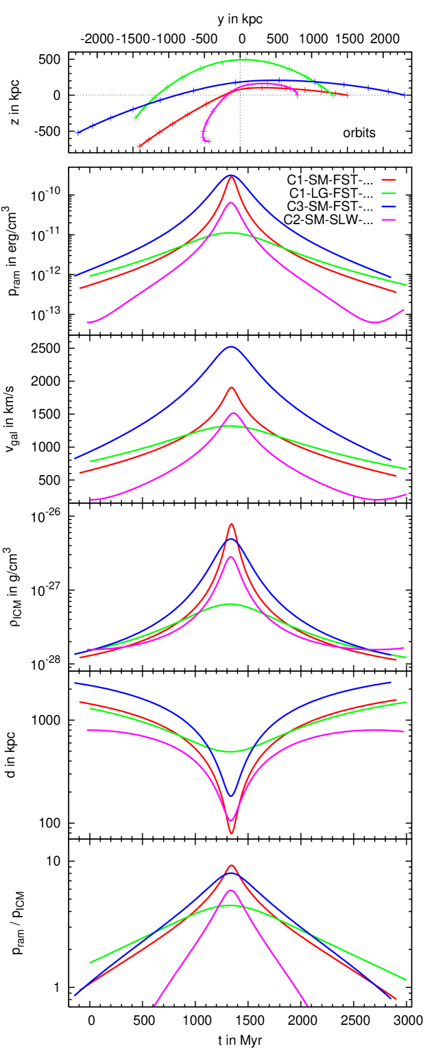
Figure 2: Summary of galaxy orbits for our simulations. The top panel shows the orbits, which are in the $y$-$z$-plane. Crosses mark the position of the galaxy in intervals of $250\,\textrm{Myr}$. The next panels show the temporal evolution of ram pressure, $p_{\mathrm{ram}}$, galaxy velocity, $v_{\mathrm{gal}}$, ICM density along orbit, $\rho_{\mathrm{ICM}}$, distance to cluster centre, $d$, and ratio between ram pressure and local ICM pressure, $p_{\mathrm{ram}}/p_{\mathrm{ICM}}$. For an explanation of the labels see text.

Three of these orbits are highly radial, whereas the fourth has a large impact parameter. The labels of the runs represent the cluster (C+number), small or large impact parameter (SM or LG), fast or slow galaxy (FST or SLW), inclination (F for near face-on, M for medium, E for near edge-on; FE for first near face-on but then near edge-on, etc.). In all cases, the galaxy orbits in the $y$-$z$-plane. Figure 3 gives a sketch of the orbital plane and galaxy orbit in the simulation box.

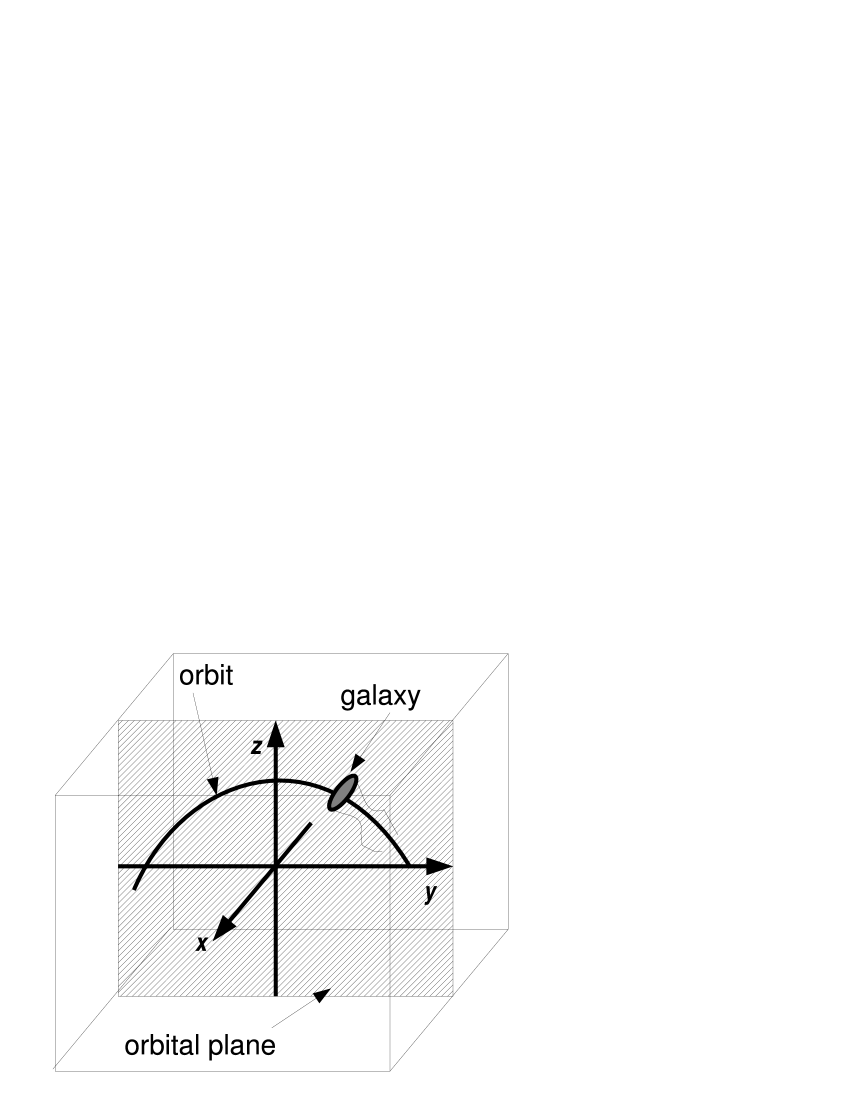
Figure 3: Sketch showing the position of the orbital plane in the simulation box. Throughout this work, we use two lines-of-sight (LOS) to view the galaxy: along the $x$-axis (towards negative direction), which means the LOS is perpendicular to the orbital plane; and along the $z$-axis (towards negative direction), which means the LOS is in the orbital plane.

Table 2 lists the simulation runs and the amount of lost gas according to paper I.

Table 2: List of runs. Run labels code the cluster (C+number), small or large impact parameter (SM or LG), fast or slow galaxy (FST or SLW), inclination (F for near face-on, M for medium, E for near edge-on; FE for first near face-on but then near edge-on, etc.). Initial galaxy coordinates $x_{\mathrm{gal}}{}_{0}$ and $z_{\mathrm{gal}}{}_{0}$ are always zero, $y_{\mathrm{gal}}{}_{0}$ is given in the second column. The third column lists the initial galaxy velocity. The fourth and fifth columns list the impact parameter and velocity, respectively. The inclination listed in the sixth column is the angle between the galaxy’s rotation axis and the $y$-axis. The seventh column states the fraction of lost gas according to paper I.

label	$y_{\mathrm{gal}}{}_{0}$	initial	impact	impact	incli-	fraction
	in	velocity	parameter	velocity	nation	of lost
	kpc	in $\,\textrm{km}\,\textrm{s}^{-1}$	in kpc	in $\,\textrm{km}\,\textrm{s}^{-1}$	in o	gas
C1-SM-FST-MF	1500	$(0,-600,100)$	79	1904	$-30$	100%
C1-SM-FST-E	$\cdot$	$\cdot$	$\cdot$	$\cdot$	$80$	100%
C1-LG-FST-MF	1300	$(0,-600,500)$	492	1320	$-30$	85%
C1-LG-FST-EF	$\cdot$	$\cdot$	$\cdot$	$\cdot$	$-60$	72%
C1-LG-FST-FE	$\cdot$	$\cdot$	$\cdot$	$\cdot$	$45$	77%
C2-SM-SLW-FME	800	$(0,0,200)$	105	1516	$30$	86%
C2-SM-SLW-EMF	$\cdot$	$\cdot$	$\cdot$	$\cdot$	$-60$	90%
C2-SM-SLW-MFM	$\cdot$	$\cdot$	$\cdot$	$\cdot$	$-20$	95%
C3-SM-FST-MF	2300	(0,-800,200)	182	2524	30	100%

3 Results

As the galaxy moves through the cluster, the ram pressure stripped gas forms a tail behind the galaxy. Some slices in the orbital plane showing the colour-coded gas density can be found in paper I and in Fig. 20. ISM densities in the tail are around $10^{-26}\,\textrm{g}\,\textrm{cm}^{-3}$ close to the galaxy ($\sim 20\,\textrm{kpc}$ distance from galaxy centre) and decrease to a few $10^{-28}\,\textrm{g}\,\textrm{cm}^{-3}$ at larger distances ($50\,\textrm{kpc}$).

3.1 Projected densities

Figures 4, 5 and 6 show snapshots of the projected ISM density for several runs.

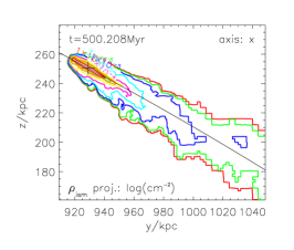
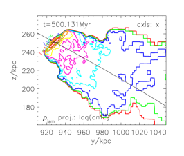
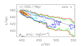
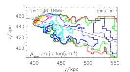
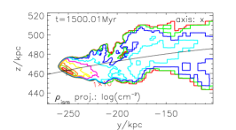
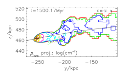
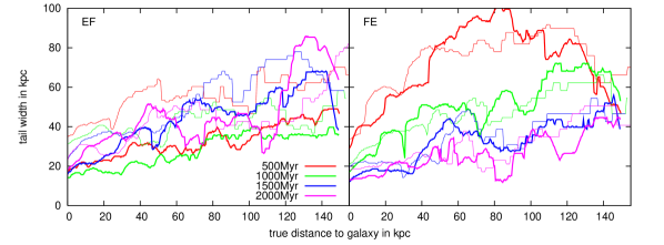
Figure 4: Projected galactic gas density for runs C1-LG-FST-EF (left column) and C1-LG-FST-FE (right column; same orbit, different inclination). Lowest contour is $10^{-6}\mathrm{g}\,\,\textrm{cm}^{-2}\hat{=}6.0\cdot 10^{17}\,\,\textrm{cm}^{-2}$. The contour spacing is half an order of magnitude. The time of each panel is denoted in its upper left corner. The label “axis: x” means the projection is done along $x$-axis, which means perpendicular to the galaxy’s orbital plane in our simulations (see Fig. 3). The galactic orbit is marked by the black line. The plus-sign marks the galactic centre. The coordinates at the axes are in the cluster-centric system. The bottom row displays the tail width as a function of distance to the galaxy at different time-steps as measured in the snapshots. Same colours are for the same time (see legend), thin lines are for projection along grid’s $z$-axis, thick lines for projection along $x$-axis (like this Figure).

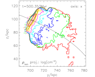
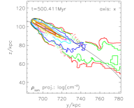
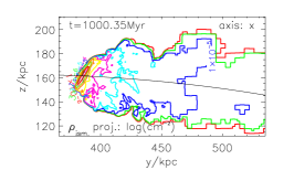
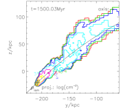
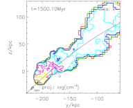
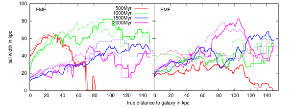
Figure 5: Same as Fig. 4 but for runs C2-SM-SLW-FME (left column) and C2-SM-SLW-EMF (right column).

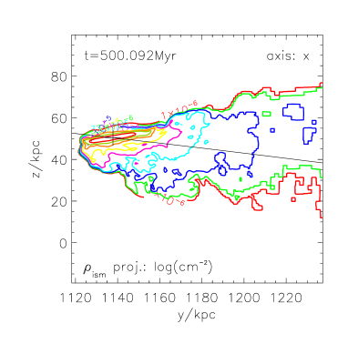
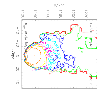
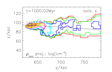
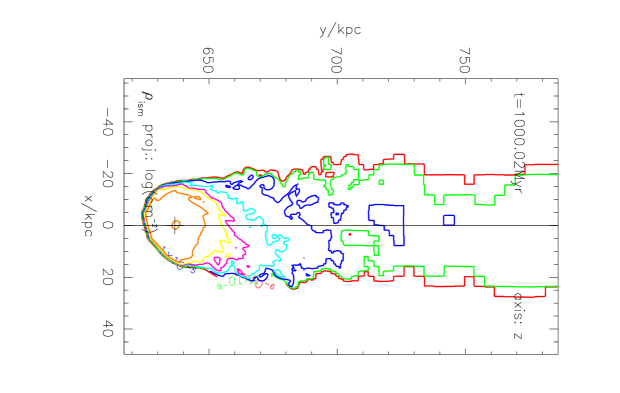
Figure 6: Like Fig. 4, but for run C1-SM-FST-E. Here, the lhs column shows the projection along the grid’s $x$-axis, and the rhs column shows projections along the grid’s $z$-axis.

Each figure is for a different orbit. In Figs. 4 and 5, the columns compare cases with different inclination but identical orbit. Figure 6 compares two different lines-of-sight (LOS) for the same run. The bottom rows of Figs. 4 and 5 summarise the temporal evolution of the tail width as a function of distance to galaxy (see discussion below).

The tails of stripped gas stretch along the galaxy’s orbit. Three features are prominent in nearly all snapshots: the tails show a flaring width, they oscillate along the orbit, and are densest close to the galaxy. Details of the structure depend on the galaxy’s current inclination and the stripping stage. In the following subsections, we describe different aspects of the tails.

3.1.1 Tail length

Typical column densities are a few $10^{19}\,\,\textrm{cm}^{-2}$ near the galaxy and $\sim 2\cdot 10^{18}\,\,\textrm{cm}^{-2}$ at large distances ($>100\,\textrm{kpc}$). A typical column density sensitivity limit for current HI observations is $10^{19}\,\,\textrm{cm}^{-2}$. Thus, we will define the length of the tail as the extent of the light blue contour ($\sim 2\cdot 10^{19}\,\,\textrm{cm}^{-2}$) behind the galaxy. In this sense, a typical tail length is $40\,\textrm{kpc}$. Tails of this length can be found at early times ($\lesssim 1\,\textrm{Gyr}$) of simulations C1-LG-FST-…(two top rows of Fig. 4), in runs C1-SM-FST-…(Fig. 6) and at early times ($\lesssim 1\,\textrm{Gyr}$) of run C3-SM-FST-MF. We wish to draw attention to the fact that at these moments the galaxy is still far, namely 400 kpc to 1 Mpc, from the cluster centre. In the Coma-like cluster C3 (run C3-SM-FST-MF), at $t=500\,\textrm{Myr}$, the galaxy is even $1800\,\textrm{kpc}$ from the cluster centre, and still shows a $50\,\textrm{kpc}$ long tail. Shorter tails are found during the first Gyr of runs C2-SM-SLW-…(Fig. 5). The longest tails are found during peri-centre passage of the same run, they extend to beyond $150\,\textrm{kpc}$. Also the snapshots at $1.5\,\textrm{Gyr}$ of runs C1-LG-FST-…reveal tails of $\sim 100\,\textrm{kpc}$ length, although – due to the large impact parameter of this orbit – also in this case the galaxy is still more than $400\,\textrm{kpc}$ from the cluster centre.

The length of the tail is influenced mainly by two parameters: the ram pressure and the galaxy’s velocity. The ram pressure determines how much gas the galaxy loses, whereas the orbital velocity determines over which volume the lost gas is spread. Clearly, high ram pressures lead to a high mass loss rate. However, as high ram pressures are usually associated with high velocities, the stripped gas is also distributed over a larger orbital length or volume. These two parameters can be combined into the mass loss per orbital length, which is the crucial quantity that characterises many tail properties.

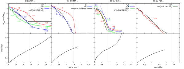
Figure 7: Evolution of gas disc mass as a function of distance covered by the galaxy (top row). Each column is for one orbit (see title of column). The colours code runs with different inclinations, see legend. The thin vertical lines mark the peri-centre passage. The bottom row displays the relation of time and covered distance. We applied piecewise linear fits to the gas disc mass as a function of covered distance. Each piece is labelled with its slope in $10^{6}M_{\sun}/\,\textrm{kpc}$.

Figure 7 displays the evolution of the remaining gas disc mass for all runs as a function of distance covered by the galaxy. The slope of these functions is the mass loss per orbital length. We fitted them piecewise with linear functions. Each piece is labelled with its slope in $10^{6}M_{\sun}/\,\textrm{kpc}$. The mass loss per orbital length ranges between a little below $10^{6}M_{\sun}/\,\textrm{kpc}$ to about $7\cdot 10^{6}M_{\sun}/\,\textrm{kpc}$. Interestingly, this quantity is largest in runs C2-SM-SLW-…during the peri-centre passage, although the ram pressure along most parts of this orbit is smaller than for all other orbits. Even during peri-centre passage, the ram pressure for this orbit is the second lowest. Here, the low orbital velocity causes a high mass loss per orbital length. The case of the Coma-like cluster C3 illustrates the opposite extreme of the same issue: Here the ram pressure is always higher than in all other runs, but the high orbital velocity of the galaxy leads to only a medium mass loss per orbital length.

Figure 8: Tail length versus mass loss per orbital length. We define the tail length as the extent of the light blue contour ($\sim 2\cdot 10^{19}\,\,\textrm{cm}^{-2}$) behind the galaxy. See also text (Sect. 3.1.1).

As expected, we find that the mass loss per orbital length correlates with the tail length (see Fig. 8). However, additional effects like the tail width play a role and lead to some scatter in this relation. Also a projection non-perpendicular to the galaxy’s direction of motion can enhance the projected density of the tail while making it appear shorter.

3.1.2 Tail width

According to simple analytical estimates (Landau & Lifschitz 1991), the width, $w$, of the wake behind a body moving through a fluid scales with distance to the body, $d$, as $\sqrt{d}$ in the case of a laminar flow and as $d^{1/3}$ in the case of a turbulent flow. In our simulations, the flow is clearly turbulent. More precisely, at large distances behind the body, the width of the wake scales as

$$w\sim 2\left(\frac{Fd}{\rho U^{2}}\right)^{1/3},$$ (2)

where $F$ is the drag force the body experiences, $\rho$ is the density of the fluid and $U$ is the flow velocity. The drag force can be written as $F=0.5c_{\mathrm{w}}A\rho U^{2}$, where $c_{\mathrm{w}}$ is the drag coefficient and $A$ the cross-section of the body. This leads to

$$w \sim 2\left(0.5c_{\mathrm{w}}Ad\right)^{1/3}$$ (3)

$$= 50\,\textrm{kpc}\left(\frac{c_{\mathrm{w}}}{1}\right)^{1/3}\left(\frac{r}{10\,\textrm{kpc}}\right)^{2/3}\left(\frac{d}{100\,\textrm{kpc}}\right)^{1/3},$$

where we have inserted values typical for our case. Here, $r$ is the radius of the remaining gas disc.

In our simulations, tail widths range between 20 to 50 kpc at a distance of $\sim 25\,\textrm{kpc}$ to the galaxy centre and 30 to 80 kpc at a distance of $\sim 100\,\textrm{kpc}$ to the galaxy centre. Near the galaxy, the tail width is similar to the galaxy’s cross-section with respect to the ICM wind direction. In an order-of-magnitude comparison, the simulation results match the analytical expectation. However, a direct application of the analytical scaling relation to our simulations is not possible, as in our simulations many assumptions that went into the analytical relation are not fulfilled: The flow past the galaxy is not static but, both, flow density and velocity change, the body (the galactic gas disc) varies in size. Furthermore, here we are interested in the wake close to the body and not far away from it. Thus it is not reasonable to fit the $d^{1/3}$ law to the galaxy’s tail.

Nonetheless, in order to quantify the flaring ratio of the tails, we applied linear fits to the tail widths as a function of distance to the galaxy, where examples are given in the bottom rows of Figs. 4 and 5. We fixed the $y$-axis cut to the galaxy’s width and fitted the slope to the data. This slope is the flaring ratio.

For each run, we have derived the flaring ratio for two lines-of-sight: once along the grid’s $x$-axis and once along the grid’s $z$-axis. The $x$-axis is always perpendicular to the galaxy’s orbit, whereas the $z$-axis is in the galaxy’s orbital plane.

Figure 9: Comparison of measured tail flaring ratios along the two different line-of-sights: perpendicular to the orbital plane and in the orbital plane. For point symbols see legend. For the definititon of the flaring ratio see text, Sect. 3.1.2.

Figure 9 demonstrates that the flaring ratios of the tails are generally independent of the direction of the line-of-sight. The only exceptions are some of the early ($t=500\,\textrm{Myr}$) snapshots, where the galaxy’s remaining gas disc is still large.

Figure 10: Tail flaring ratios as a function of inclination angle (top panel), as a function of galaxy diameter (second panel), as a function of galactic cross-section $A=\pi r_{\mathrm{disc}}^{2}\cos(i)$ (third panel), as a function of the galaxy’s velocity (fourth panel), and as a function of ram pressure (bottom panel). For point symbols see legend. For the definititon of the flaring ratio see text, Sect. 3.1.2.

Figure 10 displays the dependence of the flaring ratio on several quantities. For high ram pressures and high galaxy velocities, the flaring ratios are rather small, which reflects that for these cases the gas disc is already stripped heavily and thus is small. For smaller velocities and ram pressures, the flaring ratios show a large scatter. In addition to this, figure 10 displays the dependence of the flaring ratio on the galaxy’s inclination with respect to the ICM wind direction (top panel) and to the galaxy’s current diameter (second panel). Both plots reveal correlations in the sense that galaxies moving near face-on (small inclination angle) and galaxies with large diameters produce tails with stronger flaring. The only “exceptions” are again the early cases ($t=500\,\textrm{Myr}$). Combining these two correlations, we plotted the flaring ratios over the galaxy’s cross-section, $A=\pi r_{\mathrm{disc}}^{2}\cos(i)$, with respect to the ICM wind direction, where $r_{\mathrm{disc}}$ is the radius of the remaining gas disc. This plot reveals a clear correlation that small cross-sections lead to little flaring and vice versa. A galaxy can have a small cross-section either if it is already heavily stripped or if it is moving near edge-on. The latter cases are especially interesting. If such a galaxy is seen perpendicular to the disc, the tail is broader than if it is seen edge-on. However, the flaring for both line-of-sights is small. This reflects the known dynamics of turbulent wakes: according to Eq. 3, at a given distance, $d$, behind an object, the flaring of the wake scales as $\frac{\partial w}{\partial d}\propto A^{1/3}$, i.e. the wakes of larger objects show stronger flaring. As emphasized above, however, several assumptions that went into Eq. 3 are not fulfilled in our simulations, thus there is little hope of recovering the $A^{1/3}$ relation. We only find that a larger galactic crossection leads to stronger flaring. Nonetheless, these characteristics suggest that the flaring is determined by the turbulence in the ICM flow past the galaxy.

Effects commonly seen in simulations of harassment and tidal interactions are tilts and warps of the galactic discs (e.g. Moore et al. 1998; Mastropietro et al. 2005). These may change the orientation of the galactic disc, i.e. stars and gas, continuously. This differs from what we have assumed here. However, the effect of the cluster’s tidal field is strong only near the cluster centre, where the gas disc is already heavily ram pressure stripped. Of course interactions with other cluster galaxies may modify the gravitational potential of both galaxies and thus also influence the ram pressure stripping efficiency and characteristics of the wake. In this work here, we have isolated the effect of ram pressure stripping.

The description of the tail widths above considered the full tails. If we again adopt a column density limit of $\sim 10^{19}\,\,\textrm{cm}^{-2}$ (light blue contour), the tail flaring is much less pronounced, often not even detectable. Generally, then the tail widths are similar to the cross-section of the remaining as disc.

3.1.3 Mass distribution along the tail

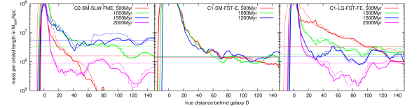
Figure 11: Galactic gas mass per orbital length as a function of distance to the galaxy for three exemplary runs. Each panel is for one run (see legends), the line colours code different time-steps, see also legends. The thin horizontal lines mark the predicted mass per orbital length as derived in Fig. 7.

Fig. 11 shows the galactic gas mass per orbital length as a function of distance to the galaxy, $D$, for three exemplary cases: we have integrated the projected gas densities perpendicular to the galaxy’s current direction of motion. As the orbits are only slightly curved, for the $150\,\textrm{kpc}$ behind the galaxy, this corresponds to very good approximation to an integration perpendicular to the orbit. The peak at $D=0$ is the gas still trapped in the galaxy. With increasing $D$, the mass per orbital length decreases and often saturates at $D\sim 70\,\textrm{kpc}$. However, this general behaviour is superimposed with substantial substructure. Especially in the tails at early simulation times ($t=500\,\textrm{Myr}$), the mass per orbital length does not saturate but continues to decrease.

The gas mass per orbital length should record the gas loss history of the galaxy. In Fig. 7 we have applied piecewise linear fits to the evolution of the galaxies’ gas disc masses as functions of covered distance. The slopes give the mass loss per orbital length and thus should be the same as the gas mass per orbital length in the tails. To compare both quantities, we have plotted the mass losses per orbital length as derived from Fig. 7 as thin horizontal lines in Fig. 11, where the colours code the time-steps according to the legend. Indeed, when the mass per orbital length saturates, it saturates at approximately the level marked by the thin horizontal lines. There are several reasons for the differences between the derived mass loss per orbital length and observed gas mass per orbital length: First of all, the mass loss per orbital length is no constant but also varies on short time- and length-scales. Secondly, the stripped gas has to be accelerated away from the galaxy, which also influences the gas distribution along the tail. Moreover, gas can be temporarily trapped in turbulent eddies, which places it in a position that cannot be predicted by the mass loss and acceleration.

3.2 Velocities in the wakes

Some slices in the orbital plane showing the gas density and the velocity field can be found in Fig. 20. The ICM is flowing around the gas disc. In cases where the galaxy moves supersonically, a bow shock is prominent. In the wake, the velocities are generally smaller than the ICM wind velocity. Additionally, the velocity field shows a turbulent structure.

Figures 12 to 14 summarise the information about the velocity in the wakes for some exemplary cases. For an ISM-density-weighted random subset of grid cells we calculate $v_{\mathrm{par}}$, the velocity component anti-parallel to the galaxy’s direction of motion, $(v_{x}{}_{\mathrm{gal}},v_{y}{}_{\mathrm{gal}},v_{z}{}_{\mathrm{gal}})$. We also calculate $v_{\mathrm{perp}}$, the component perpendicular to $v_{\mathrm{par}}$. By definition, $v_{\mathrm{perp}}$ is always positive. Both velocity components are plotted as a function of distance to the galaxy, $D$, i.e. the projection of each grid cell’s position vector in the galactocentric frame onto $(-v_{x}{}_{\mathrm{gal}},-v_{y}{}_{\mathrm{gal}},-v_{z}{}_{\mathrm{gal}})$. Additionally, we show the velocity component along the grid’s $x$-axis, $v_{x}$, which in our simulations is always perpendicular to the galaxy’s orbital plane. All velocity components are given in the galaxy’s rest frame, where the galaxy’s motion translates into an ICM wind flowing past the galaxy.

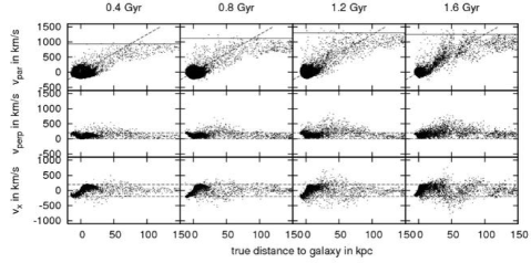
Figure 12: Three different velocity components in the galaxy’s tail, as a function of distance to the galaxy. For run C1-LG-FST-EF. The top row shows the velocity component along the tail. The middle row shows the component perpendicular to the galaxy’s direction of motion, and the bottom row the component along the grid’s $x$-axis, i.e. perpendicular to the galaxy’s orbital plane. Each column is for one time-step, as indicated. The velocities are given in the galactic rest frame. An ISM density-weighted random subset of grid cells is shown.
The solid horizontal lines in the top row panels mark the current ICM wind velocity, i.e. the negative of the galaxy’s current velocity. An identical diagonal dashed line is plotted in the top row panels in order to aid the eye to compare the slope of the velocity gradient. The horizontal lines in the middle row panels mark 0 and $200\,\textrm{km}\,\textrm{s}^{-1}$, the horizontal lines in the bottom row panels mark $\pm 200\,\textrm{km}\,\textrm{s}^{-1}$.

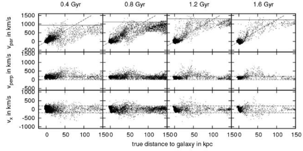
Figure 13: Same as Fig. 12, but for run C1-LG-FST-FE.

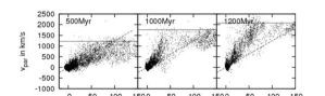
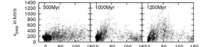
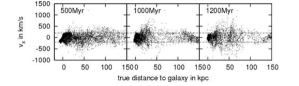
Figure 14: Same as Figs. 12, but for run C3-SM-FST-MF.

3.2.1 Velocity component anti-parallel to $\vec{v}_{\mathrm{gal}}$

The overall structure of the $v_{\mathrm{par}}$-plots is the same for all runs and all time-steps. The gas in the galactic disc appears as a blob between $D=\pm 20\,\textrm{kpc}$ and $v_{\mathrm{par}}=\pm 200\,\textrm{km}\,\textrm{s}^{-1}$, which is due to the disc’s rotation. With increasing distance to the galaxy, $v_{\mathrm{par}}$ increases towards the ICM wind velocity, which reflects the acceleration of the stripped gas by the ICM wind. At a distance of about 80 to $100\,\textrm{kpc}$ behind the galaxy, the acceleration of the stripped gas is completed, $v_{\mathrm{par}}$ does not increase any further. For a fixed distance to the galaxy, the velocity range in the tail is large. Inside the galactic disc, a width of $400\,\textrm{km}\,\textrm{s}^{-1}$ is expected due to the rotation. This behaviour is also reflected in the $v_{\mathrm{par}}$-plots. In the region where the stripped gas is accelerated, the velocity width is larger than this, it can reach $1000\,\textrm{km}\,\textrm{s}^{-1}$. Beyond distances of $\sim 40\,\textrm{kpc}$ behind the galaxy, the velocity width decreases. At distances beyond $100\,\textrm{kpc}$, the velocity width is again 400 to $500\,\textrm{km}\,\textrm{s}^{-1}$ and remains constant.

We have marked the current ICM wind velocity (or orbital velocity of the galaxy) in each plot by a horizontal line. Only very few grid cells reach $v_{\mathrm{par}}$ above this line, which is not surprising, as the ICM wind cannot accelerate gas beyond its own velocity. The acceleration of the stripped gas always proceeds in a rather similar fashion. We have plotted the same dashed diagonal line in all plots in order to aid the eye to compare the slope of $v_{\mathrm{par}}$ between different snapshots. The slope of the dashed line is representative for snapshots with ram pressures around $10^{-12}\,\textrm{erg}\,\textrm{cm}^{-3}$. For stronger ram pressures, which are also associated with higher orbital velocities, the slope is somewhat larger, for weaker ram pressures somewhat smaller. Especially for the later time-steps of run C3-SM-FST-MF (Fig. 14), where the orbital velocity is much larger than in the other cases, the velocity slope along the tail is steeper. The large velocity width in the tail near the galaxy is caused by a superposition of several processes. Firstly, also here the velocities originating from the rotation of the gas disc add to the velocity width. Secondly, denser ISM clouds need a longer time to be accelerated, while less dense structures are accelerated more easily. A third effect is the turbulence in the wake. As in our simulations the spatial resolution beyond $150\,\textrm{kpc}$ from the galactic centre is limited to $15\,\textrm{kpc}$, these simulations cannot provide reliable information beyond this distance.

We observe some occasional backfall of stripped gas well before the ram pressure peak. The backfall is temporal and becomes evident as negative $v_{\mathrm{par}}$ closely behind galaxy (e.g. early panels of Fig. 13), and as local maxima/plateaus in temporal evolution of gas mass in disc region (see paper I, or Fig. 7). A corresponding feature is evident in earlier simulations with constant ICM wind. There, the gas disc mass as a function of time shows a local maximum or plateau immediately after the instantaneous stripping phase (e.g. grid codes: Marcolini et al. 2003; Roediger & Hensler 2005; Roediger & Brüggen 2006, but also in SPH: Schulz & Struck 2001). Of couse, this feature is only observable if the evolution of the model galaxy was followed for a sufficiently long time. However, this backfall is not observed in all runs, but mainly while the galaxy moves near face-on. While the galaxy moves near edge-on, hardly any backfall is observed. Thus we conclude that the temporal backfall in our simulations is caused by the turbulent flow around the remaining gas disc. Also the shape of the galaxy’s total potential supports such this backfall behaviour, as, in the face-on case, the ram pressure meets the strongest gravitational restoring force a few kpc behind the disc plane (see e.g. Schulz & Struck 2001; Roediger & Hensler 2005; Jachym et al. 2007, but it is also the case for our model galaxy).

3.2.2 Velocity component perpendicular to $\vec{v}_{\mathrm{gal}}$

Velocities perpendicular to galaxy’s direction of motion, $v_{\mathrm{perp}}$, can be due to the disc’s rotation as well as the ICM flow around the galaxy. Moreover, turbulence in the wake adds to $v_{\mathrm{perp}}$. The component $v_{\mathrm{perp}}$ causes the tail flaring.

If all three sources were responsible for the tail flaring, we should observe that in cases where the remaining gas disc is still large but the galaxy is moving edge-on, the flaring differs between LOS perpendicular and parallel to the galactic disc. If such a galaxy is seen face-on, the rotation and the ICM flow around the galaxy contribute to the velocity component perpendicular to the LOS and tail direction. In contrast, if such a galaxy is seen edge-on, neither ICM flow nor rotation contribute to the velocity component perpendicular to the LOS and tail direction. Thus, one could expect that the tail flaring should appear stronger in the case where the galaxy is seen face-on than in the case where the galaxy is seen edge-on. However, we observe similar flaring ratios for both LOS. Thus we can conclude that mainly turbulence causes the flaring.

The velocities perpendicular to the galaxy’s direction of motion range between 0 and up to $700\,\textrm{km}\,\textrm{s}^{-1}$. In near edge-on cases, $v_{\mathrm{perp}}$ ranges only between 0 and $500\,\textrm{km}\,\textrm{s}^{-1}$. The range of $v_{\mathrm{perp}}$ is also smaller for small ram pressures and galaxy velocities. This behaviour corresponds to the rate of tail flaring. Again we observe that in cases where the galaxy’s cross-section is large, the wake is more turbulent.

The velocity component along the grid’s $x$-axis, $v_{x}$, is always perpendicular to the orbital plane and thus perpendicular to the galaxy’s direction of motion. However, unlike $v_{\mathrm{perp}}$, it does not only contain information about the amplitude of the perpendicular velocity components, but also directional information. It often shows an oscillating behaviour, which causes the oscillation of the galactic tails along the orbits as described in Sect. 3.1. These oscillations resemble von-Karman vortex streets.

The amplitude of the turbulence in the wakes seen in our simulations is comparable to the ICM turbulence generated by other processes: e.g. Norman & Bryan (1999), Dolag et al. (2005) and Vazza et al. (2006) find turbulent velocities due to structure formation and subclump infall of some $100\,\textrm{km}\,\textrm{s}^{-1}$. Kim (2007) find that gravitational wakes of galaxies produce turbulence at a level of $\lesssim 220\,\textrm{km}\,\textrm{s}^{-1}$.

3.3 Distribution of stripped material throughout the cluster

The galaxy’s gas loss history is reflected in the distribution of the stripped gas throughout the galaxy cluster. In Fig. 15 we show this distribution for the orbit C1-LG-FST-…for two different galaxy inclinations.

 

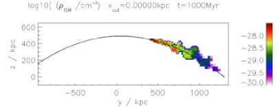
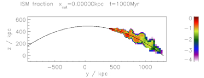
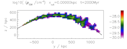
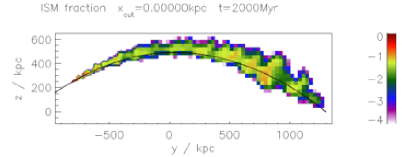
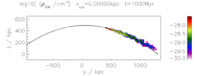
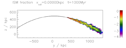
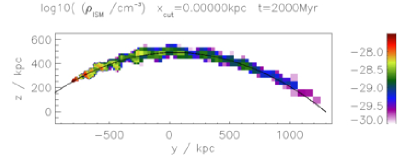
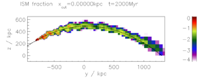
Figure 15: Slices in the orbital plane showing the ISM distribution throughout the cluster colour-coded for different time-steps. The two top rows are for run C1-LG-FST-FE, the two bottom rows for run C1-LG-FST-EF. The lhs column displays the density of (stripped) ISM, $\rho_{\mathrm{ISM}}$, the rhs column displays the local ISM fraction, $\rho_{\mathrm{ISM}}/\rho_{\mathrm{ICM}}$. The black line marks the galaxy’s orbit.

Clearly, different inclinations lead to different gas loss histories and thus differing distributions of the stripping gas throughout the cluster. In order to describe the distribution of stripped gas along the galaxy’s orbit, we have calculated the ISM mass inside a sphere of radius $150\,\textrm{kpc}$ around each orbit point. Dividing this mass by the orbit length inside the sphere (which is $300\,\textrm{kpc}$) yields the local ISM mass per orbital length, averaged over $300\,\textrm{kpc}$. This quantity is plotted in Fig. 16 for different time-steps of simulation run C1-LG-FST-MF.

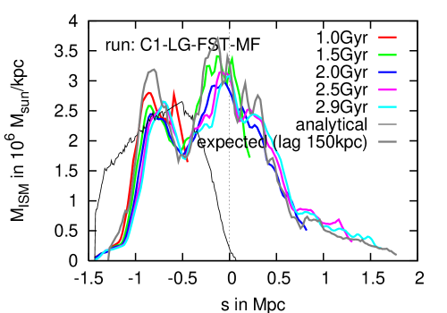
Figure 16: Distribution of stripped gas along orbit at different time-steps for run C1-LG-FST-MF, averaged over $300\,\textrm{kpc}$. The thin black line is the prediction based on the analytical estimate of the stripping mass (see paper I). The gray line is the prediction based on the numerical result of the bound gas mass as a function of covered distance – however – shifted by $150\,\textrm{kpc}$ along the orbit. The zero-point of the $x$-axis is shifted to peri-centre passage.

Figure 17 displays the same quantity for all runs at a fixed time-step $t=2\,\textrm{Gyr}$.

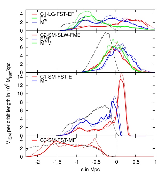
Figure 17: Distribution of stripped gas along orbit at $t=2\,\textrm{Gyr}$, averaged over $300\,\textrm{kpc}$. Each panel is for one orbit, different inclinations are colour-coded (see legend). For each run, the thick line is the distribution of stripped gas as seen in the simulation. The thin line of the same colour is the prediction based on the numerical result of the bound gas mass as a function of covered distance – however – shifted by $150\,\textrm{kpc}$ along the orbit. The black line is the prediction from the analytical estimate. The zero-point of the $x$-axis is shifted to peri-centre passage.

We had to use a rather large averaging length due to the large wake width at large distances from the galaxy. Using a smaller smoothing length would have meant to miss some gas.

Figure 17 again reflects the fact that the amount of gas that the galaxy deposits locally depends on its mass loss per orbital length. E.g. in the simulation run corresponding to the bottom panel, the ram pressure is always larger than in the other simulations. However, here the galaxy is also moving faster than in all other simulations, and thus spreads its gas over a larger volume and larger orbital length. Consequently, the local amount of stripped gas is not higher than in the other simulations.

The amount of stripped gas found per orbital length has to be closely linked to the galaxy’s mass loss rate per orbital length discussed in connection with Fig. 7. In our simulations, we know the amount of ISM bound to the galaxy potential. If we assume that the stripped gas is deposited into the ICM exactly where it is lost, we can predict the expected ISM mass per orbital length. The gray line in Fig. 16 shows this function, however, shifted by $150\,\textrm{kpc}$ along the orbit. The thin lines in Fig. 17 show the same for the other runs. This means that the stripped gas is deposited into the ICM about $150\,\textrm{kpc}$ from the position where it was lost from the galaxy’s potential. In other words, the stripped gas follows the galaxy for about $150\,\textrm{kpc}$ before finding its final position in the cluster centre. Thus, in our simulations, the stripped gas is deposited into the ICM rather locally. We have also plotted the prediction for the distribution of the stripped gas based on the analytical estimate of the galaxy’s stripping radius (Gunn& Gott criterion, see paper I). If the galaxy lost its gas according to this criterion and if the stripped gas remained where it was lost, its distribution along the orbit would be as shown by the thin black lines in Figs. 16 and 17. In most cases, the simulations and the analytical prediction differ, according to the simulations the stripped gas is deposited later along the orbit.

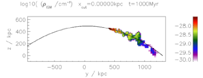
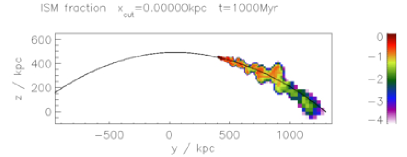
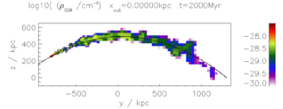
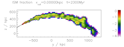
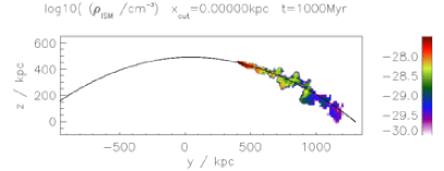
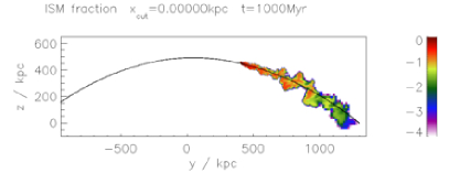
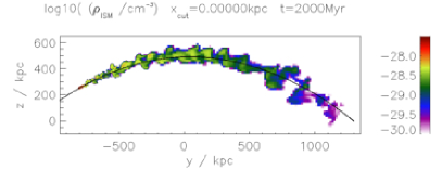
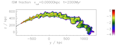
Figure 19: Same as Fig. 15, but for run C1-LG-FST-MF. The two top rows are for a resolution as described in Sect. 2.1, in the two bottom rows the resolution is improved by a factor 2 everywhere.

We need to point out that results regarding the distribution of the stripped gas throughout the cluster are approximations, as in our simulations we have limited the spatial resolution outside $150\,\textrm{kpc}$ from the galaxy. However, according to the velocity plots, the deceleration of the stripped gas is finished within $150\,\textrm{kpc}$ from the galaxy. Moreover, if the spatial resolution is improved by a factor of 2 throughout the simulation box, the results are very similar (see Figs. 19 and 23). Thus, we conclude that our results do not suffer from insufficient resolution.

Typical ISM fractions in the wake $\sim 100\,\textrm{kpc}$ behind the galaxy are around 20%. Assuming an ISM metallicity of about solar and an ICM metallicity of about 0.4 solar, this leads to a metallicity of 0.52 in the wake. For an ISM metallicity of twice solar and ICM metallicity of 0.2 solar, the resulting metallicity in the wake is 0.56 solar. In how far the wake is detectable in X-ray metal maps depends also on the temperature in the wake. As we do not know the temperatures in the wake, we cannot make predictions at this point.

Obviously, RPS is a source of metals for the ICM. The cumulative effect of the whole galaxy population on the ICM is studied by Domainko et al. (2006) and compared to other enrichment processes by Schindler et al. (2005); Kapferer et al. (2007); Moll et al. (2007). Here, the enrichment by RPS is modelled by applying the classical Gunn & Gott criterion to the galaxy particles and thus calculating a mass loss rate for each galaxy. The gas predicted to be stripped is added locally to the ICM. In this treatment, galaxies lose gas only as long as the ram pressure is increasing, only on their way towards the cluster centre. Our simulations show that galaxies lose their gas somewhat more slowly than predicted, stripped gas is also found along the orbit after peri-centre passage. These characteristics could lead to a slightly broader distribution of ram pressure induced metals in the ICM.

3.4 Energy input into the ICM

The galaxy carries a large amount of kinetic energy. The ram pressure working on the gas disc is associated with a drag force that decelerates the galaxy. This mechanism provides a heating source for the ICM. The energy lost by the galaxy can be thermalised in the ICM either via decaying turbulence or via viscosity. Here we want to investigate the relevance of this heating mechanism.

A body of mass, $M$, and cross-section, $A$, that is subject to the ram pressure, $p_{\mathrm{ram}}$, experiences the drag force, $F_{\mathrm{D}}=-p_{\mathrm{ram}}A$ and the associated deceleration

$$a_{\mathrm{D}}=-\frac{p_{\mathrm{ram}}A}{M}.$$ (4)

The energy loss rate for this body is

$$\frac{\mathrm{d}}{\mathrm{d}t}E_{\mathrm{kin}}=-Mva_{\mathrm{D}}=-vp_{\mathrm{ram}}A.$$ (5)

The more relevant quantity in our context is the energy loss per orbital length,

$$\frac{\mathrm{d}}{\mathrm{d}s}E_{\mathrm{kin}}=F_{\mathrm{D}}=-p_{\mathrm{ram}}A$$ (6)

We can compare this quantity to the local turbulent energy per orbital length in the galaxy’s wake, which is

$$\frac{\mathrm{d}}{\mathrm{d}s}E_{\mathrm{turb}}=\frac{1}{2}\rho_{\mathrm{ICM}}v_{\mathrm{turb}}^{2}A_{\mathrm{wake}},$$ (7)

where $v_{\mathrm{turb}}$ is the typical turbulent velocity in the wake and $A_{\mathrm{wake}}$ the wake’s cross-section. Assuming that the loss of kinetic energy is converted locally into turbulence, energy conservation requires that these two quantities are the same. Making use of the relation $p_{\mathrm{ram}}=\frac{1}{2}c_{\mathrm{w}}\rho_{\mathrm{ICM}}v_{\mathrm{gal}}^{2}$, this leads to the following relation between the body’s (the galaxy’s) orbital velocity, $v_{\mathrm{gal}}$, and the ratio of the cross-sections of the body and the wake:

$$\frac{v_{\mathrm{turb}}}{v_{\mathrm{gal}}}=\sqrt{c_{\mathrm{w}}\frac{A}{A_{\mathrm{wake}}}}.$$ (8)

As usual, $c_{\mathrm{w}}$ is the drag coefficient that parametrises the response of the body in question to a flow, it depends on the body’s shape and surface properties. For a disc-like body we have $c_{\mathrm{w}}\sim 1$ if the disc is moving face-on. In case of our galaxy, the ratio between the gas disc’s cross-section and the wake’s cross-section is $\sim 4$ to 9. For a typical orbital velocity of $1000\,\textrm{km}\,\textrm{s}^{-1}$ this leads to turbulent velocities of the order of $400\,\textrm{km}\,\textrm{s}^{-1}$, which is what we observe in our simulations.

Now we want to address the question of the relevance of this process as a heating mechanism for the ICM. Given that the analytical estimate for the stripping radius gives a reasonable result for a large range of situations (see paper I), we can use $A=\pi r_{\mathrm{disc}}^{2}$ as an estimate for the galaxy’s cross-section, where $r_{\mathrm{disc}}$ is the stripping radius derived from the analytical estimate. Furthermore, we assume that the kinetic energy lost by the galaxy is available for ICM heating locally. Thus, we can calculate the local heat gain per orbital length to be

$$\frac{\mathrm{d}}{\mathrm{d}s}E_{\mathrm{heat}}=-\frac{\mathrm{d}}{\mathrm{d}s}E_{\mathrm{kin}}=p_{\mathrm{ram}}\pi r_{\mathrm{disc}}^{2}.$$ (9)

However, not all of this energy can really be used to heat the ICM. Some part is consumed in removing the galaxy’s gas disc from the galactic potential. The total binding energy of the gas disc is $\sim 1.5\cdot 10^{58}\,\textrm{erg}$, and it scales approximately linear with disc radius with a slope of $\frac{\mathrm{d}E_{\mathrm{pot}}}{\mathrm{d}r_{\mathrm{disc}}}\sim 8\cdot 10^{56}\,\textrm{erg}/\,\textrm{kpc}$. Thus, the amount of energy consumed in this process per orbital length is

$$\frac{\mathrm{d}}{\mathrm{d}s}E_{\mathrm{pot}}=\frac{\mathrm{d}E_{\mathrm{pot}}}{\mathrm{d}r_{\mathrm{disc}}}\frac{\mathrm{d}r_{\mathrm{disc}}}{\mathrm{d}s}\approx 8\cdot 10^{56}\frac{\,\textrm{erg}}{\,\textrm{kpc}}\frac{\mathrm{d}r_{\mathrm{disc}}}{\mathrm{d}s},$$ (10)

where the change of disc radius per orbital length, $\frac{\mathrm{d}r_{\mathrm{disc}}}{\mathrm{d}s}$, is also given by the analytical estimate. Figure 18 compares the energy input into the ICM due to the drag deceleration of the galaxy and the energy lost by the removal of the stripped gas from the galaxy’s potential for the four different orbits.

Figure 18: Energy gain for the ICM along the orbit. For four different orbits (see label in upper right corners). The zero-point of the $x$-axis is shifted to peri-centre passage.

The energy budget is given locally along the galaxy’s orbit, as energy per orbital length. Clearly, the input of energy into the ICM due to the galaxy’s drag deceleration dominates. The radiative loss from the ICM by thermal bremsstrahlung was not considered here as due to its strong dependence on ICM density it can be relevant only close to cluster centres.

In order to judge the importance this energy gain for the ICM, we can compare the original amount of thermal energy along the wake, $eA_{\mathrm{wake}}$, with this heat gain. The thermal energy density, $e$, can be expressed in terms of the sound speed, $c_{\mathrm{s}}$:

$$e\approx\rho_{\mathrm{ICM}}c_{\mathrm{s}}^{2},$$ (11)

where we have made use of the fact that in our case $(\gamma-1)\gamma\approx 1$. Thus, the ratio of heat gain and thermal energy is

$$\frac{\mathrm{d}E_{\mathrm{heat}}/\mathrm{d}s}{eA_{\mathrm{wake}}}=0.5c_{\mathrm{w}}\frac{v_{\mathrm{gal}}^{2}A_{\mathrm{disc}}}{c_{\mathrm{s}}^{2}A_{\mathrm{wake}}}$$ (12)

Usually, the wake diameter is at least a factor of 2 larger than the diameter of the gas disc. In our simulations, the orbital velocity reaches Mach numbers of 2 only in the cluster centre. Thus, the energy gain by ram pressure deceleration would correspond to a local energy (and temperature) increase by a factor of 2 at maximum. In principle, the heating could be strongest near the cluster centre as there the galaxy moves fastest, but due to ram pressure stripping also here the gas disc is rather small or even gone completely. Thus, the process of drag deceleration is unlikely to be able to stop cooling flows. In summary, this means that ICM heating due to ram pressure deceleration of galaxies is not expected to play a crucial role. This conclusion is not surprising if we remember that the ICM temperature as well as the galaxies’ velocity dispersion are determined by the same gravitational potential and the total mass of ICM is larger or comparable to the total mass of all galaxies. This means that the total amount of thermal energy in the ICM is comparable or larger than the total kinetic energy of all cluster galaxies. Moreover, the galaxies lose only a fraction of their kinetic energy by drag deceleration. In our calculation we have also assumed that the galaxy is moving (near) face-on. For galaxies moving near edge-on, the drag force as well as the heating rate will be somewhat smaller.

Another process to convert the kinetic energy of the galaxies into thermal energy of the ICM is dynamical friction (e.g. Kim et al. 2005 and references therein). The decelerating force working on a galaxy of mass, $M_{\mathrm{gal}}$ as it moves through a homogeneous medium of density, $\rho$, with velocity, $v_{\mathrm{gal}}$, is

$$F_{\mathrm{DF}}=\frac{4\pi\rho G^{2}M_{\mathrm{gal}}^{2}}{v_{\mathrm{gal}}^{2}}I,$$ (13)

According to Ostriker (1999), the efficiency factor $I$ summarises the dependence on Mach number and impact parameters, it is in the range of 1 to 10. The density, $\rho$, of the surrounding medium is the ICM density plus the DM density. As an approximation, we will use $I=1$ and $\rho=10\rho_{\mathrm{ICM}}$, and a total galaxy mass of $5\cdot 10^{11}M_{\sun}$. Then we can calculate the dynamical friction force, which is equivalent to the galaxy’s energy loss per orbital length. The result is also shown in Fig. 18. The energy available from dynamical friction is comparable to the energy available from hydrodynamical drag. However, dynamical friction is stronger in cluster centres. At first glance, also the hydrodynamical drag should be strong in cluster centres as the ram pressure is highest there, but the high ram pressure causes ram pressure stripping and thus small galactic gas discs and, consequently, small drag forces.

Given the deceleration by dynamical friction, $a_{\mathrm{DF}}=F_{\mathrm{DF}}/M_{\mathrm{gal}}$, we can estimate how much the galaxy gets decelerated during one orbit:

$$\Delta v = a_{\mathrm{DF}}\Delta t$$ (14)

$$= 18\,\textrm{km}\,\textrm{s}^{-1}\left(\frac{\rho}{10^{-26}\,\textrm{g}\,\textrm{cm}^{-3}}\right)\left(\frac{M_{\mathrm{gal}}}{5\cdot 10^{11}M_{\sun}}\right)$$

$$\left(\frac{v_{\mathrm{gal}}}{1000\,\textrm{km}\,\textrm{s}^{-1}}\right)^{-2}\left(\frac{I}{1}\right)\left(\frac{\Delta t}{1\,\textrm{Gyr}}\right),$$

which implies that deceleration due to dynamical friction is negligible as long as only the first orbit is concerned. As the strength of the hydrodynamical drag force is similar to the dynamical friction, the same applies to the hydrodynamical drag.

4 Discussion

4.1 Summary of tail properties

The overall picture of ram pressure induced galactic tails as derived from our simulations can be summarised as follows (we use the galactic rest frame). There are two main processes:

• The ICM wind accelerates the stripped gas along the orbit away from the galaxy. The acceleration is finished $\sim 100\,\textrm{kpc}$ behind the galaxy.

• Additionally, mainly turbulence in the wake leads to a flaring of the tail. The turbulence and hence flaring ratios depend on the galaxy’s cross-section with respect to the ICM wind direction: Small cross-sections lead to little flaring, large cross-sections lead to stronger flaring.

This leads to the following characteristics:

• The tails of stripped gas stretch along the galaxy’s orbit. They oscillate slightly along the orbit and show a flaring width.

• Local ISM densities in the tail are around $10^{-26}\,\textrm{g}\,\textrm{cm}^{-3}$ close to the galaxy ($\sim 20\,\textrm{kpc}$ distance from galaxy centre) and a few $10^{-28}\,\textrm{g}\,\textrm{cm}^{-3}$ at larger distances ($50\,\textrm{kpc}$).

• Projected ISM densities are a few $10^{19}\,\,\textrm{cm}^{-2}$ near the galaxy and $\sim 2\cdot 10^{18}\,\,\textrm{cm}^{-2}$ at large distances (50 to $100\,\textrm{kpc}$).

• The density and length of the tail (for a given column density limit) are set by the galaxy’s mass loss per orbital length.

• Widths range between 20 to 50 kpc at a distance of $\sim 25\,\textrm{kpc}$ to the galaxy centre and 30 to 80 kpc at a distance of $\sim 100\,\textrm{kpc}$. If we adopt a column density limit of $\sim 2\cdot 10^{19}\,\,\textrm{cm}^{-2}$, the tail width is similar to the galaxy’s apparent cross-section with respect to ICM wind direction and does not show flaring.

• For the same column density limit, typical tail lengths are $40\,\textrm{kpc}$. Even in compact clusters like Virgo, such tails can also be found for galaxies that are still 0.5 to 1 Mpc from the cluster centre. In extended clusters like Coma, 40 kpc long tails can be found even at cluster-centric distances of 1800 kpc. For high mass losses per orbital length (e.g. a passage close to the cluster centre with moderate velocity), tail lengths can reach $150\,\textrm{kpc}$.

• At a distance of $\sim 70\,\textrm{kpc}$, the galactic gas mass per orbital length along the tail converges roughly to the galaxy’s mass loss per orbital length. Typical values are around $3\cdot 10^{6}M_{\sun}/\,\textrm{kpc}$. The mass per orbital length along the tail can also be derived for observed galaxies. In order to disentangle a galaxy’s mass loss history from this quantity, the tail needs to be observed to at least this distance behind the galaxy. With typical tail widths of $\sim 50\,\textrm{kpc}$, a sensitivity limit of a few $10^{18}\,\,\textrm{cm}^{-2}$ is required.

4.2 Limits of this work

In our simulations, we neglected cooling and thermal conduction. Thus, we are unable to predict the temperature in the wakes and the spectral range in which they are observable. Recent observations of long galactic tails in the Virgo cluster (Oosterloo & van Gorkom 2005, Chung et al. 2007) suggest that the stripped gas could remain cool for a few $100\,\textrm{Myr}$. In contrast, the long X-ray tail observed by Sun et al. (2006) – if it is ram pressure induced – suggests that at least some part of the stripped gas is heated to higher temperatures. Cooling may also affect the stripping efficiency (Mastropietro et al. 2005). However, in order to include cooling in a propper way, also star formation and supernova feedback would have to be modelled, i.e. the multiphase nature of the ISM would have to be taken into account. This is beyond the scope of this paper but will be a highly relevant subject of future work.

Cooling may also influence the morphology of the tails. Dense regions may cool and contract further, thus forming a clumpy tail. However, for the densities ($<10^{-26}\,\textrm{g}\,\textrm{cm}^{-3}$) and temperatures ($\sim 10^{7}\,\textrm{K}$) in the wakes in our current simulations the cooling time is at least several 10 Myr and thus comparable or longer than the dynamical timescale.

Moreover, Vietri et al. (1997) have shown that in the case of dense cool clouds in moving though the warm ISM, radiative cooling can prevent the disruption of these clouds by the KH instability. The instability of shear flows at the boundary of an object that moves through some fluid are the main reason for the generation of a turbulent wake. Thus, one may wonder if the presence of cooling could also prevent the generation of turbulence in the wake of our model galaxies. One major difference to the work of Vietri et al. (1997) is, however, the density and temperature range under consideration. In the simulations of Vietri et al. (1997), the cooling times inside the clouds are always much shorter that the dynamical timescale. This is not the case in the ICM, here cooling times are at least comparable to the dynamical timescale. Moreover, a close inspection of the snapshots presented in Vietri et al. (1997) reveals that the flow of the hot gas still shows some eddies, even when cooling is included. In a similar context, Vieser & Hensler (2007) have studied the influence of thermal conduction on the survival of cool, dense clouds. They find that the interplay of cooling and thermal conduction can stabilise the clouds against KH instability. Again, the densities and temperatures studied are different from our case. Thus, the influence of cooling and thermal conduction on the dynamics of the wakes is another important task for future studies.

We also neglected viscosity in our simulations. The amplitude of viscosity in the ICM is still a matter of debate (e.g. Reynolds et al. 2005; Ruszkowski et al. 2004). We note that the same applies to the heat conduction. A higher viscosity prevents turbulent motions in the wakes and thus would suppress tail flaring. Consequently, in a viscous ICM, ram pressure induced tails would be narrower than the ones in our simulations. Moreover, the velocity width across the tail would be smaller. A comparison between viscous and non-viscous RPS simulations and detailed observations could help to measure the viscosity of the ICM.

Despite the many possibilites to improve our model, this model provides an important starting point to compare theory and observations.

4.3 Comparison with other simulations

4.3.1 Constant ICM wind simulations

Roediger et al. (2006) have studied galactic wakes in ram pressure simulations using a constant ICM wind. Also these simulations showed the acceleration of the stripped gas away from the galaxy and the flaring of the tails. However, in these simulations, the tails were generally broader than the ones presented here. In static wind simulations, the increase of $v_{\mathrm{par}}$ due to acceleration takes somewhat longer. However, the constant wind simulations suffered from the difficulty that the flow had to be initialised at full strength, which is artificial. Concerning the dynamical aspect, the cluster crossing simulations presented here are by far more realistic.

4.3.2 Sticky-particle simulations

Also the sticky-particle simulations of Vollmer et al. (see Sect. 1) describe RPS of galaxies on cluster orbits. According to their simulations, regarding the particle density, the stripped gas often forms a dense arm that originates at one edge of the galaxy and is much narrower than the galaxy’s cross-section. The low particle density extent of the tail has the same width as the galaxy and shows some flaring depending on stripping geometry. In their work, they usually concentrated on the gas distribution close to the galaxy, thus there are no predicted HI maps for long tails.

For galaxies moving near edge-on, the sticky particle simulations predict a characteristic backfall of stripped gas some time after peri-centre passage. We do not observe such a backfall in any of our simulations, which is most likely due to the fact that our model clusters and thus ram pressure peaks are somewhat broader than the cases studied by Vollmer et al. (2001). However, we observe a temporal backfall of gas for near face-on cases while the galaxy approaches the cluster centre. This backfall is caused by the turbulent velocity structure in the wake and can thus not be present in the sticky-particle simulations.

4.3.3 SPH simulations

Jachym et al. (2007) presented SPH simulations of RPS of disc galaxies on cluster orbits. Also in their work, internal processes in the ISM (cooling, star formation, feedback) were neglected; the ISM was treated isothermally, while the ICM was treated adiabatically. Additionally, they restricted the ram pressure interaction to the inner $300\,\textrm{kpc}$ (in diameter) of the cluster. Most of their model clusters were more compact than our model clusters. This fact and the restriction to the inner cluster part may be the reasons why also this group observes reaccretion or backfall of stripped gas after peri-centre passage, while our simulations do not show such a behaviour. The galactic wakes in these simulations also seem to differ from the wakes in our simulations. However, a detailed comparison is difficult as they mostly show only the first $20\,\textrm{kpc}$ behind the galaxy. In the simulations of Jachym et al. (2007), the opening angle of the tail is influenced mainly by the ram pressure strength: when the ram pressure is still low and the galaxy moving slowly, the tails appear to be flaring strongly, and with increasing ram pressure and galactic velocity the opening angle decreases and remains moderate after peri-centre passage. Apparently, the tail width at a distance of 100 kpc behind the galaxy is less than 50 kpc, which is not much more than the original diameter of the galaxy. Additionally, the velocity in the wake shows mainly a slow motion in ICM wind direction and only very small velocity components perpendicular to the galaxy’s direction of motion. Thus, the tail opening angle in these simulations seems not to be caused by a significant perpendicular velocity component as in our case. It mainly reflects that first the outer parts of the gas disc are stripped, and, as the galaxy approaches the cluster centre, gas from smaller and smaller radii is stripped. The authors also mention that the stripped gas tails behind the galaxy with a fraction of the galaxy’s velocity and that the tails remain denser than the local ICM by a factor of a few. Our wakes behave differently. The stripped gas remains within $\sim 150\,\textrm{kpc}$ from where it was stripped. Also the density in the tails of our galaxies are much lower, it exceeds 1.2 times the local ICM density only very close to the galaxy (see Fig. 15 and 19).

The different behaviour in the simulations of Jachym et al. (2007) has several reasons: The ram pressure interaction is described differently, their effective resolution in the tails may be lower than in our simulations, most of their clusters are more compact and have a lower ICM density, and they restricted the ICM-ISM interaction to the inner 300 kpc of the cluster.

4.4 Comparison with observations

4.4.1 Long HI tails in cluster outskirts

Chung et al. (2007) have searched for HI tails in the Virgo cluster. Of the $\sim 50$ targeted spiral galaxies, 7 revealed long one-sided HI tails. Surprisingly, these galaxies are at projected cluster-centric distances of $0.6$ to $1\,\textrm{Mpc}$. For their sensitivity limit of $\sim 2\cdot 10^{19}\,\,\textrm{cm}^{-2}$, the tail lengths are $\sim 30$ to $40\,\textrm{kpc}$, while tail widths are similar to the cross-section of the remaining gas disc with respect to tail direction. The column density decreases gradually along the tail. Chung et al. (2007) estimated likely ram pressures and gravitational restoring forces for the galaxies. Comparing the two forces, they found that 5 of these 7 galaxies could indeed suffer RPS.

In our simulations, we have not modelled the Virgo cluster directly, but our cluster C1 is also a compact cluster. In the literature, different parameters for the ICM distribution in the Virgo cluster are given (see Fig. 1). For cluster-centric radii of 0.5 to 1 Mpc, our cluster C1 is a factor of about 3.6 denser than the version used in Vollmer et al. (2001), but agrees well with the parameters given by Matsumoto et al. (2000). Thus, we consider a comparison of the tails observed by Chung et al. (2007) with our simulated tails in cluster C1 reasonable.

Adopting a column density limit comparable to the sensitivity limit of the observations, our simulations are able to produce tails with similar characteristics regarding length, width and structure also at large distances to the cluster centre (e.g. first row of Fig. 4 and first two rows of Fig. 6). However, not all simulated galaxies at large cluster-centric distances show long tails. In the first row of Fig. 5, the tails are rather short, because here the ram pressure is very small due to the small orbital velocity of this galaxy. Thus, we conclude that it is possible that the tails observed by Chung et al. (2007) are produced by ram pressure stripping although the galaxies are still a large distance from the cluster centre. However, these galaxies need to have a substantial velocity component, i.e. about $1000\,\textrm{km}\,\textrm{s}^{-1}$, in the plane of the sky. Not all galaxies at large cluster-centric distances observed by Chung et al. (2007) show long tails. The reason can simply be that not all galaxies have a sufficient velocity component in the plane of the sky. We expect that in more extended clusters like Coma, long ram pressure induced tails can be found at even larger distances to the cluster centre.

Our velocity plots (Figs. 12 to 14) are the analogue to the position-velocity diagrams (PVD) presented by Chung et al. (2007). However, given the sensitivity limit of observations, only the densest features of our velocity diagrams will be observable. In the observations presented by Chung et al. (2007), the gas tails appear as a “hook” that is attached to one edge of the galaxy and shows a slight slope towards the galaxy’s systemic velocity. This hook has a small velocity width, $\lesssim 200\,\textrm{km}\,\textrm{s}^{-1}$, in some cases even less. If this was the whole velocity width of the tail, this would be surprising, as one would expect a velocity width like in the galactic disc ($\sim 400\,\textrm{km}\,\textrm{s}^{-1}$).

In our simulations, we can observe a similar “hook”-feature in our $v_{x}$-plots, if we consider only densest parts, in cases where the galaxy is not moving close to face-on. Also here, the velocity width in the hook is only $\lesssim 200\,\textrm{km}\,\textrm{s}^{-1}$, which agrees with the observations. In the simulations, the “hook” is not as long as in observations. This feature is generated by the fact that in these cases the gas loss happens mainly at one side of the galaxy, namely the part of the leading edge where the galaxy rotates along with the wind. Also most galaxies with tails observed by Chung et al. (2007) are not moving close to face-on. However, in our simulations, this hook feature is not as clear as in the observations. Moreover, nearly all of the tailed galaxies observed by Chung et al. (2007) show this hook, whereas in our simulations the hook appears only occasionally and along preferable line-of-sights. In general, in the PVDs of our simulations, the tail is much more diffuse than the observed ones. A reason for this difference could be that real RPS does not proceed as turbulent as in our simulations, but that viscosity leads to a smoother flow.

We note that in the observed galaxies, in almost all cases the velocity gradient along the tail/hook is not only towards the cluster mean, but also towards the galaxy’s systemic velocity. Moreover, some of the observed galaxies have a very small radial velocity with respect to the Virgo cluster mean, so that at maximum a weak velocity gradient along the tail could be expected, if the gradient is due to the acceleration of the stripped gas away from the galaxy. We speculate that the gradient in the tail does not simply show the acceleration of stripped gas away from the galaxy, but that the deceleration of the gas disc’s rotational component along the tail plays a crucial role.

4.4.2 The case of NGC 4388

The Virgo spiral galaxy NGC 4388 seems to be an excellent example of a ram pressure stripped galaxy. It is known to have a $\sim 35\,\textrm{kpc}$ long tail of ionised gas (Yoshida et al. 2002, 2004). Additionally, Oosterloo & van Gorkom (2005) have found a $\sim 120\,\textrm{kpc}$ long HI tail associated with this galaxy.

NGC 4388 has a high radial velocity of $1400\,\textrm{km}\,\textrm{s}^{-1}$ (see Vollmer & Huchtmeier 2003 and references therein) with respect to the cluster mean. Given its long tail in projection, it also must have significant velocity component in the plane of the sky. A reasonable assumption is that the velocity component in the sky is comparable to the radial one, which would lead to a total velocity of $\sim 2000\,\textrm{km}\,\textrm{s}^{-1}$ in the Virgo cluster rest frame, which is rather high. However, assuming a much smaller component in the plane of the sky would increase the true length of the HI tail a lot. Our current assumption already results in a true length of the HI tail of $\sim 1.5\times 120\,\textrm{kpc}=180\,\textrm{kpc}$.

A reasonable value for the local ICM density at the position of NGC 4388 is a few $10^{-28}\,\textrm{g}\,\textrm{cm}^{-3}$. With a likely velocity of about $2000\,\textrm{km}\,\textrm{s}^{-1}$, it experiences a ram pressure of about $10^{-11}\,\textrm{erg}\,\textrm{cm}^{-3}$. According to our simulations, this is enough to be stripped heavily, so regarding the degree of stripping, simulations and observations agree.

Regarding the combination of orbital velocity and local ICM density, in our simulations, there is no case directly comparable to NGC 4388. The closest our simulations get to the velocity-density combination of NGC 4388 is the peri-centre passage of runs C1-LG-FST-…or at $\sim 800\,\textrm{Myr}$ of run C3-SM-FST-MF. In both cases, the ram pressure is about $10^{-11}\,\textrm{erg}\,\textrm{cm}^{-3}$, but the orbital velocity is only slightly below $1500\,\textrm{km}\,\textrm{s}^{-1}$. In both cases, the mass loss per orbital length is about $2.7\cdot 10^{6}M_{\sun}\,\textrm{kpc}^{-1}$. Given that NGC 4388 is probably a factor of $\sim 1.4$ faster than the two mentioned examples, also the mass loss per orbital length should be a factor of $\sim 1.4$ smaller, which would lead to a less dense tail than the ones in the mentioned runs. As an opposing effect, the line-of-sight and the tail of NGC 4388 make an angle of about $45^{o}$, so that projected densities appear a factor of $1.4$ higher than they would if the line-of-sight and the tail were perpendicular to each other. Also the projected gas mass per orbital length is about $1.4$ times higher. As these two effects cancel each other, we expect column densities and gas masses per orbital length comparable to the ones in our simulations. Thus, our simulations predict that the column density in the tail near the galaxy should be near $\sim 10^{20}\,\,\textrm{cm}^{-2}$, and decrease gradually with increasing distance to the galaxy to below $\sim 10^{19}\,\,\textrm{cm}^{-2}$ at a distance of $\sim 50\,\textrm{kpc}$ or latest $100\,\textrm{kpc}$ behind the galaxy. At a distance of $\sim 100\,\textrm{kpc}$, the gas mass per orbital length should correspond to the galaxy’s mass loss per orbital length, which we estimated above to be about $3\cdot 10^{6}M_{\sun}\,\textrm{kpc}^{-1}$.

However, the tail of NGC 4388 looks different. It is densest at a distance of $\sim 100\,\textrm{kpc}$ behind the galaxy, here the column density reaches $\sim 10^{20}\,\,\textrm{cm}^{-2}$. The spatial width of this dense patch is about $5\,\textrm{kpc}$, thus this dense patch corresponds to a mass per orbital length of about $4\cdot 10^{6}M_{\sun}\,\textrm{kpc}^{-1}$. Towards the galaxy, the column density as well as the mass per orbital length decrease. In HI, the tail even shows a gap near the galaxy. In this gap, Yoshida et al. (2002) observed a plume of ionised gas. However, the total mass of this plume is only $10^{5}M_{\sun}$, which corresponds to a mass per orbital length to $3\cdot 10^{4}M_{\sun}\,\textrm{kpc}^{-1}$ and is much less than we expected. Thus, the distribution of stripped gas along the tail differs from what we expect.

The width of the tail shows some flaring. In our simulations, we do not observe tail flaring in the sensitivity limit of these simulations. In the simulations, the tails show flaring only at much lower column densities.

The ionised part of the tail NGC 4388 shows a filamentary structure. On the basis of a deep spectroscopic study, Yoshida et al. (2004) derive the H$\alpha$ velocity field, which turns out to be quite complicated. The authors identify several kinematic groups among the filaments. However, they also consider significant turbulent motions possible. They argue that the kinematic structure and metallicity of the ionisation are not well-explained by a minor-merger scenario, but can be explained naturally by ram pressure stripping and an additional starburst driven superwind in the galactic nucleus. According to our simulations, turbulent motions in the tail are very likely. However, the mass of stripped gas near the galaxy is much less than we expected.

The HI tail of NGC 4388 (Oosterloo & van Gorkom 2005) remains hard to fit with the simulations also with respect to the velocity information. The velocity width of the tail is rather small over the whole length. Additionally, according to our simulations, the acceleration of the stripped gas towards the ICM velocity is finished approximately at a distance of $100\,\textrm{kpc}$ behind the galaxy. For NGC 4388, however, the velocity of at the end of the tail differs from the galaxy’s systemic velocity only by $500\,\textrm{km}\,\textrm{s}^{-1}$. According to our simulations, a value comparable to the galaxy’s radial velocity with respect to the cluster mean, $1400\,\textrm{km}\,\textrm{s}^{-1}$, would be expected.

In summary, our simulations have difficulties to explain the details of NGC 4388’s tail, where the most severe points are:

• The distribution of stripped gas along the tail differs between observations and simulations. The simulations predict much more gas near the galaxy. The mass per orbital length at a distance of $\sim 100\,\textrm{kpc}$ behind the galaxy is approximately at the expected level, however, here the gas is confined in a smaller volume than expected and thus shows higher column densities than expected.

• According to our simulations, the stripped gas should be decelerated to the cluster mean velocity at a distance of $\sim 100\,\textrm{kpc}$. According to the HI data, for NGC 4388, however, the stripped gas seems to have lost only 1/3 of the expected velocity change. In contrast to this, the H$\alpha$ tail shows a velocity gradient as expected from our simulations. Radial velocities at the end of the H$\alpha$ tail have already reached $300$ to $500\,\textrm{km}\,\textrm{s}^{-1}$. Also the turbulent structure of the H$\alpha$ velocity field is in agreement with our simulations. We note that here the HI and the H$\alpha$ data seem to be in disagreement.

There are several reasons that could cause the mismatches between the simulations and the observations. E.g. the ICM may not be smooth but inhomogeneous, and there may be ambient motions in the ICM, thus leading to a special ram pressure history of this galaxy. The Virgo spiral NGC 4522 is another example that suggests ambient motions in the ICM, as its degree of stripping implies a much stronger ram pressure than expected at its position in the cluster (Vollmer et al. 2006). Moreover, NGC 4388 has an active nucleus and a starburst driven superwind (see Yoshida et al. 2004 and references therein), which will influence the dynamics of the ICM-ISM interaction. Additionally, our simulations cannot predict the temperature of the stripped gas and are thus unable to predict in which wavelengths the stripped gas is observable. However, the close vicinity of the galaxy has been searched for ionised and neutral gas and the amounts found are significantly less than what we expect.

4.4.3 H$\alpha$ and X-ray tails

Up to date, only a few galaxies with H$\alpha$ and X-ray tails are known. There are two irregular galaxies in the cluster A 1367 that have H$\alpha$ tails of $50\,\textrm{kpc}$ and $75\,\textrm{kpc}$ length and $8\,\textrm{kpc}$ width (Gavazzi et al. 2001). The tails are straight and show some filamentary structure along the tail. Yagi et al. (2007) have observed the Coma galaxy D 100 and found an H$\alpha$ tail that is exceptionally straight and narrow ($60\,\textrm{kpc}$ long, $2\,\textrm{kpc}$ wide). The H$\alpha$ tail of NGC 4388 has been discussed above in connection with its HI tail.

Sun et al. (2006) have presented a long and narrow X-ray tail ($70\,\textrm{kpc}$ long, $7\,\textrm{kpc}$ wide) for the galaxy ESO 137-001 in the Coma-like cluster A 3627. Additionally, Sun et al. (2007) have found a $40\,\textrm{kpc}\times 4\,\textrm{kpc}$ H$\alpha$ tail for the same galaxy that coincides spatially with the X-ray tail. The mass of the X-ray tail is estimated to be $10^{9}M_{\sun}$, the H$\alpha$ tail provides another few $10^{8}M_{\sun}$. Both, the X-ray and the H$\alpha$ tail are nearly straight, although some very slight oscillation can be detected. In both wavebands, the highest emission is found near the galaxy, but there are some more brighter patches further downstream. If the brightness also traces the local gas mass, this behaviour would be expected if these tails are caused by ram pressure stripping. Also the total gas mass of the tails matches the ram pressure picture.

A characteristic feature of the observed H$\alpha$ and X-ray tails is their narrowness and straightness. Given that our simulations cannot estimate the temperature of the stripped gas, we are unable to predict the brightness distribution of our tails in H$\alpha$ or in X-rays. However, the projected density maps presented in this paper generally show much broader tails and make such narrow and straight tails difficult to understand. Although our simulations provide an important step towards a realistic description of RPS by modelling the flight through a cluster, still important physics seems to be missing.

5 Summary

We have performed 3D hydrodynamical simulations of ram pressure stripping of disc galaxies on orbits through galaxy clusters. Here we have presented a detailed study of the wakes associated with these galaxies.

For a sensitivity limit typical for current HI observations ($10^{19}\,\,\textrm{cm}^{-2}$), we find that a typical tail length in projected gas density is $40\,\textrm{kpc}$. In this sensitivity limit, the width of the tails is similar to the galaxy’s width with respect to the tail direction. Our simulations show that the density and length of the tail is not determined by the current ram pressure and thus temporal mass loss rate alone, but also by the galaxy’s velocity. These two dependencies can be summarised in the mass loss per orbital length, which is the crucial parameter that determines the tail length and density.

If we consider projected gas densities below the sensitivity limit, the tails show a flaring width, where the flaring ratio depends on the galaxy’s cross-section with respect to its direction of motion. Large cross-sections lead to strong flaring, while for small cross-sections the flaring is weak. The flaring is caused by turbulence in the galactic wakes.

The velocity in our wakes shows a significant turbulent component of a few $100\,\textrm{km}\,\textrm{s}^{-1}$. The stripped gas is fully decelerated to the ICM rest frame at a distance of $\sim 100\,\textrm{kpc}$ behind the galaxy.

We find that the stripped gas does not follow the galaxy for a long way but remains within $\sim 150\,\textrm{kpc}$ from the position where it is lost. We have investigated in how far the deceleration of the galaxy by the drag force can be a heating source for the ICM and found that no significant effect is expected.

As our simulations neglect thermal conduction, cooling and viscosity, they are unable to predict the wavelength at which the galactic wakes should be observable. Nonetheless, we compared our simulations with observations of galactic wakes.

We can reproduce tails of $40\,\textrm{kpc}$ length at cluster-centric distances between $0.5$ and $1\,\textrm{Mpc}$ in a compact cluster similar to the Virgo cluster. Thus we conclude that the galactic tails found by Chung et al. (2007) could indeed be formed by ram pressure stripping. However, our simulations have difficulties in reproducing the velocity information of these galaxies. The observations suggest that RPS proceeds less turbulent than in our simulations. Also, the structure of the wake of the Virgo spiral NGC 4388 is hard to explain by our simulations, not only due to shortcomings of our simulations, but also due to intrinsic discrepancies in this galaxy’s data. This HI “tail” may not be caused by RPS at all, or this galaxy may have experienced a complex ram pressure history. Given that our simulations cannot predict the correct gas temperatures, comparisons to the H$\alpha$ and X-ray tails are especially difficult. However, our simulations do not seem to be able to match the straightness and narrowness of these tails. Also these observations suggest that some physics that were neglected in our model, e.g. viscosity, cooling, and tidal interactions, may play an important role for the detailed structure of ram pressure stripping tails.

Appendix A Resolution

In this section, we show slices in the orbital plane that display the local gas density and the flow structure (Fig. 20), projected gas density maps (Fig. 21) and velocity plots (Fig. 22). These Figs. are for the run C1-LG-FST-MF, but once for the spatial resolution as described in Sect. 2.1, and once for a run were the spatial resolution as been improved by a factor of 2 everywhere. Figure 23 compares the distribution of stripped gas along the orbit.

In all plots, the basic structure is same for both resolutions. We conclude that our conclusions are not influenced by the resolution.

 

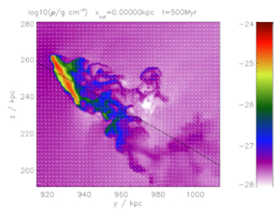
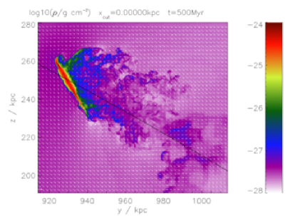
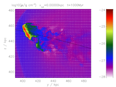
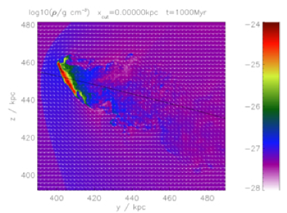
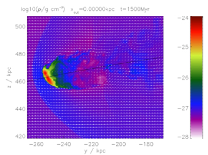
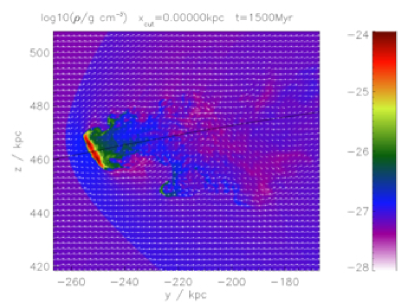
Figure 20: Slices in the orbital plane, showing the local gas density colour-coded, and the velocity field projected onto this plane by arrows, for different time-steps. For run C1-LG-FST-MF. Left column is for resolution as described in Sect. 2.1, right column is for resolution improved by a factor 2 everywhere. The black line marks the galaxy’s orbit. The velocities are shown in the galactic rest frame. The horizontal arrow in the lower left corner shows the length of the magnitude of the ICM wind at each time-step. The axis coordinates are in the cluster-centric system.

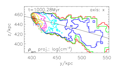
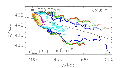
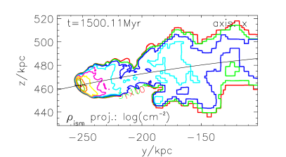
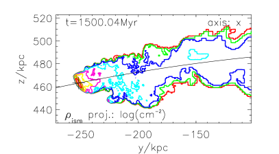
Figure 21: Same as Fig. 4 but for run C1-LG-FST-MF. The lhs column is for the resolution described in Sect. 2.1, the rhs column for a run where the resolution has been improved by a factor of 2 everywhere.

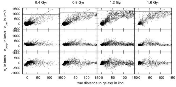
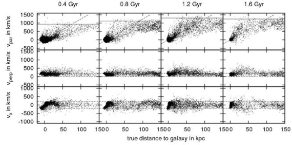
Figure 22: Same as Fig. 12, but for run C1-LG-FST-MF. Top plate is for resolution as described in Sect. 2.1, bottom plate is for run with resolution improved by a factor of 2 everywhere.

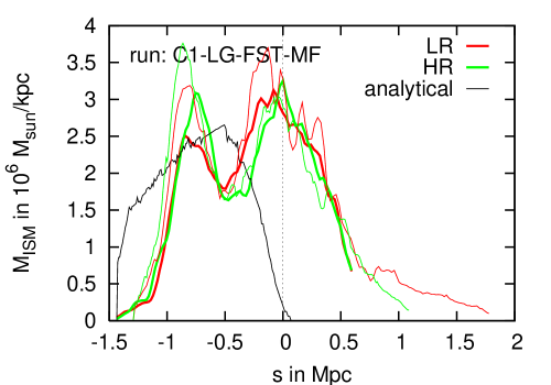
Figure 23: Distribution of stripped gas along orbit (compare to Figs. 16 and 17): for run C1-LG-FST-MF, averaged over $300\,\textrm{kpc}$, for two different resolutions. Colours code the resolution (LR is low resolution, HR is resolution improved by a factor of 2 everywhere). The thick lines are distribution as seen in the simulation. The thin coloured lines are the predictions based on the numerical result of the bound gas mass as a function of covered distance – however – shifted by $150\,\textrm{kpc}$ along the orbit. The thin black line is the prediction based on the analytical estimate of the stripping mass (see paper I). The zero-point of the $x$-axis is shifted to peri-centre passage.

References

- Abadi et al. (1999) Abadi M. G., Moore B., Bower R. G., 1999, MNRAS, 308, 947
- Brüggen & De Lucia (2007) Brüggen M., De Lucia G., 2007, MNRAS, accepted
- Chung et al. (2007) Chung A., van Gorkom J. H., Kenney J. D. P., Vollmer B., 2007, ApJ, 659, L115
- Churazov et al. (2003) Churazov E., Forman W., Jones C., Böhringer H., 2003, ApJ, 590, 225
- Cora (2006) Cora S. A., 2006, MNRAS, 368, 1540
- De Grandi et al. (2004) De Grandi S., Ettori S., Longhetti M., Molendi S., 2004, A&A, 419, 7
- Dolag et al. (2005) Dolag K., Vazza F., Brunetti G., Tormen G., 2005, MNRAS, 364, 753
- Domainko et al. (2006) Domainko W., Mair M., Kapferer W., van Kampen E., Kronberger T., Schindler S., Kimeswenger S., Ruffert M., Mangete O., 2006, A&A, 452, 795
- Fryxell et al. (2000) Fryxell B., Olson K., Ricker R., Timmes F. X., Zingale M., Lamb D. Q., MacNeice P., Rosner R., Truran J. W., Tufo H., 2000, ApJS, 131, 273
- Gavazzi et al. (2001) Gavazzi G., Boselli A., Mayer L., Iglesias-Paramo J., Vílchez J. M., Carrasco L., 2001, ApJ, 563, 23L
- Gunn & Gott (1972) Gunn J. E., Gott J. R., 1972, ApJ, 176, 1
- Jachym et al. (2007) Jachym P., Palous J., Köppen J., Combes F., 2007, A&A, 472, 5
-
Kapferer
et al. (2006)
Kapferer W., Ferrari C., Domainko W., Mair M., Kronberger T., Schindler
S., Kimeswenger S., van Kampen E., Breitschwerdt D., Ruffert M.,
2006,
aap, 447, 827 - Kapferer et al. (2007) Kapferer W., Kronberger T., Weratschnig J., Schindler S., Domainko W., E.van Kampen Kimeswenger S., Mair M., Ruffert M., 2007, A&A, 466, 813
- Kenney & Koopmann (1999) Kenney J. D. P., Koopmann R. A., 1999, AJ, 117, 181
- Kenney & Koopmann (2001) Kenney J. D. P., Koopmann R. A., 2001, in Hibbard J. E., Rupen M. P., van Gorkom J. J., eds, Gas and Galaxy Evolution Vol. 240 of ASP Conf. Ser., Environmental effects on gas and star formation in virgo cluster spiral and peculiar galaxies. ASP, San Francisco, p. 577
- Kenney et al. (2004) Kenney J. D. P., van Gorkom J. H., Vollmer B., 2004, AJ, 127, 3361
- Kim et al. (2007) Kim D., Kim E., Fabbiano G., Trinchieri G., 2007, ApJ, submitted
- Kim et al. (2005) Kim W., El-Zant A. A., Kamionkowski M., 2005, ApJ, 632, 157
- Kim (2007) Kim W.-T., 2007, ApJ, 667, L5
- Landau & Lifschitz (1991) Landau L. D., Lifschitz F. M., 1991, Lehrbuch der theoretischen Physik VI: Hydrodynamik. Akademie Verlag, Berlin
- Marcolini et al. (2003) Marcolini A., Brighenti F., A.D’Ercole 2003, MNRAS, 345, 1329
- Mastropietro et al. (2005) Mastropietro C., Moore B., Mayer L., Debattista V. P., Piffaretti R., Stadel J., 2005, MNRAS, 364, 607
- Mastropietro et al. (2005) Mastropietro C., Moore B., Mayer L., Wadsley J., Stadel J., 2005, MNRAS, 363, 509
- Matsumoto et al. (2000) Matsumoto H., Tsuru T. G., Fukazawa Y., Hattori M., Davis D. S., 2000, PASJ, 52, 153
- Matsushita et al. (2002) Matsushita K., Belsole E., Finoguenov A., Böhringer H., 2002, A&A, 386, 77
- Matsushita et al. (2003) Matsushita K., Finoguenov A., Böhringer H., 2003, A&A, 401, 443
- Mayer et al. (2006) Mayer L., Mastropietro C., Wadsley J., Stadel J., Moore B., 2006, MNRAS, 369, 1021
- Mohr et al. (1999) Mohr J. J., Mathiesen B., Evrard A. E., 1999, ApJ, 517, 627
- Moll et al. (2007) Moll R., Schindler S., Domainko W., Kapferer W., Mair M., van Kampen E., Kronberger T., Kimeswenger S., Ruffert M., 2007, A&A, accepted
- Moore et al. (1996) Moore B., Katz N., Lake G., Dressler A., Oemler A., 1996, Nature, 379, 613
- Moore et al. (1998) Moore B., Lake G., Katz N., 1998, ApJ, 495, 139
- Moore et al. (1999) Moore B., Lake G., Quinn T., Stadel J., 1999, MNRAS, 304, 465
- Norman & Bryan (1999) Norman M. L., Bryan G. L., 1999, in The Radio Galaxy Messier 87 Vol. 530 of Lecture Notes in Physics, Cluster Turbulence. Springer Verlag, Berlin, p. 106
- Oosterloo & van Gorkom (2005) Oosterloo T., van Gorkom J., 2005, A&A, 437, L19
- Ostriker (1999) Ostriker E. C., 1999, ApJ, 513, 252
- Quilis et al. (2000) Quilis V., Moore B., Bower R., 2000, Science, 288, 1617
- Reynolds et al. (2005) Reynolds C. S., McKernan B., Fabian A. C., Stone J. M., Vernaleo J. C., 2005, MNRAS, 357, 242
- Roediger & Brüggen (2006) Roediger E., Brüggen M., 2006, MNRAS, 369, 567
- Roediger & Brüggen (2007) Roediger E., Brüggen M., 2007, MNRAS, 380, 1399
- Roediger et al. (2006) Roediger E., Brüggen M., Hoeft M., 2006, MNRAS, 371, 609
- Roediger & Hensler (2005) Roediger E., Hensler G., 2005, A&A, 433, 875
- Ruszkowski et al. (2004) Ruszkowski M., Brueggen M., Begelman M. C., 2004, ApJ, 611, 158
- Schindler et al. (2005) Schindler S., Kapferer W., Domainko W., Mair M., van Kampen E., Kronberger T., Kimeswenger S., Ruffert M., Mangete O., Breitschwerdt D., 2005, A&A, 435, L25
- Schmidt et al. (2002) Schmidt R. W., Fabian A. C., Sanders J. S., 2002, MNRAS, 337, 71
- Schulz & Struck (2001) Schulz S., Struck C., 2001, MNRAS, 328, 185
- Sun et al. (2007) Sun M., Donahue M., Voit G. M., 2007, ApJ, in press
- Sun et al. (2006) Sun M., Jones C., Forman W., Nulsen P. E. J., Donahue M., Voit G. M., 2006, ApJ, 637, L81
- Sun et al. (2007) Sun M., Jones C., Forman W., Vikhlinin A., Donahue M., Voit G. M., 2007, ApJ, 657, 197
- Sun & Vikhlinin (2005) Sun M., Vikhlinin A., 2005, ApJ, 621, 718
- Tonnesen et al. (2007) Tonnesen S., Bryan G. L., van Gorkom J. H., 2007, ApJ
- Tornatore et al. (2004) Tornatore L., Borgani S., Matteucci F., Recchi S., Tozzi P., 2004, MNRAS, 349, L19
- Valdarnini (2003) Valdarnini R., 2003, MNRAS, 339, 1117
- Vazza et al. (2006) Vazza F., Tormen G., Cassano R., Brunetti G., Dolag K., 2006, MNRAS, 369, L14
- Vieser & Hensler (2007) Vieser W., Hensler G., 2007, A&A, 472, 141
- Vietri et al. (1997) Vietri M., Ferrara A., Miniati F., 1997, ApJ, 483, 262
- Vollmer (2003) Vollmer B., 2003, A&A, 398, 525
- Vollmer et al. (2004) Vollmer B., Balkowski C., Cayatte V., van Driel W., Huchtmeier W., 2004, A&A, 419, 35
- Vollmer et al. (2004) Vollmer B., Beck R., Kenney J. D. P., van Gorkom J. H., 2004, AJ, 127, 3375
- Vollmer et al. (2001) Vollmer B., Braine J., Balkowski C., Cayatte V., Duschl W. J., 2001, A&A, 374, 824
- Vollmer et al. (2001) Vollmer B., Cayatte V., Balkowski C., Duschl W. J., 2001, ApJ, 561, 708
- Vollmer et al. (1999) Vollmer B., Cayatte V., Boselli A., Balkowski C., Duschl W. J., 1999, A&A, 349, 411
- Vollmer & Huchtmeier (2003) Vollmer B., Huchtmeier W., 2003, A&A, 406, 427
- Vollmer & Huchtmeier (2007) Vollmer B., Huchtmeier W., 2007, A&A, 462, 93
- Vollmer et al. (2005) Vollmer B., Huchtmeier W., van Driel W., 2005, A&A, ??, ??
- Vollmer et al. (2000) Vollmer B., Marcelin M., Amram P., Balkowski C., Cayatte V., Garrido O., 2000, A&A, 364, 532
- Vollmer et al. (2006) Vollmer B., Soida M., Otmianowska-Mazur K., Kenney J. D. P., van Gorkom J. H., Beck R., 2006, A&A, 453, 883
- Wang et al. (2004) Wang Q. D., Owen F., Ledlow M., 2004, ApJ, 611, 821
- Yagi et al. (2007) Yagi M., Komiyama Y., Yoshida M., Furusawa H., Kashikawa N., Koyama Y., Okamura S., 2007, ApJ, 660, 1209
- Yoshida et al. (2004) Yoshida M., Ohyama Y., Iye M., Aoki K., Kashikawa N., Sasaki T., Shimasaku K., Yagi M., Okamura S., Doi M., Furusawa H., Habame M., Kimura M., Komiyama Y., Miyazaki M., Miyazaki S., Nakata F., Ouchi M., Sekiguchi M., Yasuda N., 2004, AJ, 127, 90
- Yoshida et al. (2002) Yoshida M., Yagi M., Okamura S., Aoki K., Ohyama Y., Komiyama Y., Yasuda N., Iye M., Kashikawa N., Doi M., Furusawa H., Hamabe M., Kimura M., Miyazaki M., Miyazaki S., Nakata F., Ouchi M., Sekiguchi M., Shimasaku K., Ohtani H., 2002, ApJ, 567, 118
- Zaritski et al. (2004) Zaritski D., Gonzalez A. H., Zabludoff A. I., 2004, ApJ, 613, L93