Disclosing hidden information in the quantum Zeno effect:
Pulsed measurement of the quantum time of arrival

Abstract

Repeated measurements of a quantum particle to check its presence in a region of space was proposed long ago (G. R. Allcock, Ann. Phys. 53, 286 (1969)) as a natural way to determine the distribution of times of arrival at the orthogonal subspace, but the method was discarded because of the quantum Zeno effect: in the limit of very frequent measurements the wave function is reflected and remains in the original subspace. We show that by normalizing the small bits of arriving (removed) norm, an ideal time distribution emerges in correspondence with a classical local-kinetic-energy distribution.

I Introduction

The theoretical treatment of time observables is one of the important loose ends of quantum theory. Among them the time of arrival (TOA) has received much attention lately dam02 ; rus02 ; alo02 ; ON03 ; gal04 ; rus04 ; bon04 ; gdme05 ; LL ; as06 ; heg06 ; gas06 ; heg07 ; man07 ; tor07 ; goz07 , for earlier reviews see ML00 ; MSE02 . A major challenge is to find the connection between ideal TOA distributions, defined for the particle in isolation, formally independent of the measurement method, and operational ones, explicitly dependent on specific measurement models and procedures. It is important to know, for example, what exactly a given operational procedure is measuring, or if and how a given ideal quantity may or may not be obtained with a particular experiment.

Modern research on the quantum TOA owes much to the seminal work by Allcock Allcock . Looking for an ideal quantum arrival-time concept, he considered that arrival-time measuring devices should rapidly transfer any probability that appears at $x>0$ ($x=0$ being the “arrival position”) from the incident channel into various orthogonal and time-labeled measurement channels. As a simple model to realize this basic feature he proposed a pulsed, periodic removal, at time intervals $\delta t$, of the wave function for $x>0$, while the $x<0$ region would not be affected, see Fig. 1. A similar particle removal would provide the distribution of first arrivals for an ensemble of classical, freely-moving particles as $\delta t\to 0$.

The difficulties to solve the corresponding mathematical problem lead Allcock to study instead a different, continuous model with an absorbing imaginary potential in the right half-line, $-iV_{0}\Theta(x)$, $V_{0}>0$, to simulate the detection. He argued that the two models should lead to similar conclusions with a time resolution of the order $\delta t$ in the chopping model or $\hbar/2V_{0}$ in the complex potential model. He then solved the Schrödinger equation with the complex potential and noticed that for $V_{0}\gg|E|_{max}$, where $E_{max}$ is a maximum relevant energy in the wave packet,

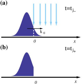
Figure 1: Schematic representation of the time of arrival measurement by periodic projection of the wave function onto the subspace $x<0$ at times $t_{j}$, $j=..,-1,0,1,..$ separated by $\delta t$. Figures (a) and (b) represent two instants immediately before and after the elimination of norm at $x>0$.

the apparatus response vanishes, $-\delta N/\delta t\to 0$, with $N=\langle\psi|\psi\rangle$, because of quantum mechanical reflection. This is one of the first discussions of the quantum Zeno effect, although it was not known by this name at that time. Eight years later Misra and Sudarshan MS77 generalized this result studying the passage of a system from one predetermined subspace to its orthogonal subspace: the periodic projection method in the limit $\delta t\to 0$ was presented as a natural way to model a continuous measurement, however it did not lead to a time distribution of the passage but to its suppression MS77 . This lack of a “trustworthy algorithm” to compute TOA and related distributions prompted them to put in doubt the completeness of quantum theory and has been much debated since then, see hom97 ; fac01 ; kos05 for review. For the specific case of a projection onto a region of space, as in the TOA procedure proposed by Allcock, several works have later emphasized that, in the limit of infinitely frequent measurements, the resulting “Zeno dynamics” in the original subspace corresponds to hard wall (Dirichlet) boundary conditions fac01a ; fac04 ; exn05 .

Allcock discarded the short $\delta t$ (or high $V_{0}$) limit as useless, and examined the other limit where the measurement may be expected to be $V_{0}$-independent, $V_{0}\ll|E_{min}|$, later on. We shall not treat this limit hereafter but, for completeness, let us briefly recall that he got the current density $J(t)$ by deconvolution of the absorbed norm with the apparatus response function,

$$J(t)=\frac{\hbar}{2m}\langle{\psi_{f}(t)}|(\widehat{k}\delta(\widehat{x})+\delta(\widehat{x})\widehat{k})|{\psi_{f}(t)}\rangle,$$ (1)

where $\widehat{k}$ and $\widehat{x}$ are the wavenumber and position operators, $m$ is the mass, and the average is computed with the freely moving wave function $\psi_{f}$. This result makes sense classically, but in quantum mechanics $J(t)$ is not positive semidefinite even for states composed only by positive momenta Allcock ; ML00 . He also got, within some approximation, a positive distribution, $\Pi_{K}(t)$, which has been later known as “Kijowski’s distribution” Kijowski74 ; ML00 ; ON03 ,

$$\Pi_{K}(t)=\frac{\hbar}{m}\langle{\psi_{f}(t)}|\widehat{k}^{1/2}\delta(\widehat{x})\widehat{k}^{1/2}|{\psi_{f}(t)}\rangle.$$ (2)

In this paper, instead of disregarding the Zeno limit because of reflection, as it is customary, we shall look at the small amount of norm $\delta N$ detected, i.e., eliminated in the projection process, and normalize,

$$\Pi_{Zeno}=\lim_{\delta t\to 0}\frac{-\delta N/\delta t}{1-N(\infty)}.$$ (3)

In this manner, a rather simple ideal quantity will emerge: there is, in other words, interesting physical information hidden behind the Zeno effect, which can be disclosed by normalization. To fulfill this program we shall put the parallelism hinted by Allcock between the pulsed measurement and the continuous measurement on a firmer, more quantitative basis.

II Zeno time distribution

We shall now define formally the pulsed and continuous measurement models mentioned above and also an intermediate auxiliary model alo02 that will be a useful bridge between the two. Ref. mug06 is followed initially although the analysis and conclusions will be quite different.

The “chopping process” amounts to a periodic projection of the wave function onto the $x<0$ region at instants separated by a time interval $\delta t$. There is nothing here beyond standard measurement theory vN . Each chopping step eliminates interference terms in the density operator between right and left components, and the right component is separated from the ensamble (detected) so that it cannot come back to the left. The wave functions immediately after and before the projection at the instant $t_{j}$, are related by $\psi(x,{t_{j}}_{+})=\psi(x,{t_{j}}_{-})\Theta(-x).$

The wave at $x>0$ may also be canceled with a “kicked” imaginary potential $\widehat{V}_{k}=\widehat{V}\delta t\,F_{\delta t}(t),$ where the subscript “k” stands for “kicked” and $F_{\delta t}(t)=\sum_{j=-\infty}^{\infty}\delta(t-j\delta t)$,

$$\widehat{V}=-i\widehat{V}_{I}=-iV_{0}\Theta(\widehat{x}),$$ (4)

provided

$$V_{0}\delta t\gg\hbar.$$ (5)

The general (and exact) evolution operator is obtained by repetition of the basic unit

$$\widehat{U}_{k}(0,\delta t)=e^{-i\widehat{H}_{0}\delta t/\hbar}e^{-i\widehat{V}\delta t/\hbar},$$ (6)

where $\widehat{H}_{0}=-(\hbar^{2}/2m)\partial^{2}/\partial x^{2}$.

For the continuous model, the evolution under the imaginary potential (4) is given by

$$\widehat{U}(0,\delta t) = e^{-i(\widehat{H}_{0}+\widehat{V})\delta t/\hbar}=e^{-i\widehat{H}_{0}\delta t/\hbar}e^{-i\widehat{V}\delta t/\hbar}$$ (7)

$$+ {\cal O}(\delta t^{2}[\widehat{V},\widehat{H}_{0}]/\hbar^{2}).$$

Comparing with Eq. (6) we see that the kicked and continuous models agree when

$$\delta t^{2}|\langle[\widehat{V},\widehat{H}_{0}]\rangle|/\hbar^{2}\ll 1.$$ (8)

At first sight a large $V_{0}\delta t/\hbar$, see Eq. (5), seems to be incompatible with this condition so that the three models would not agree mug06 . In fact the numerical calculations give a different result and show a better and better agreement between the continuous and pulsed models as $V_{0}\to\infty$ when $\delta t$ and $V_{0}$ are linked by some predetermined (large) constant $\alpha$, $\delta t=\alpha\hbar/V_{0}.$

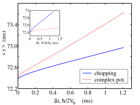
Figure 2: Average absorption times evaluated from $-dN/dt$ (normalized) for the projection method and the continuous (complex potential) model. The initial state is a minimum uncertainty product Gaussian for ²³Na atoms centered at $x_{0}=-500\mu$m with $\Delta x=23.5\mu$m and average velocity $0.365$ cm. In all numerical examples negative momentum components of the initial state are negligible.

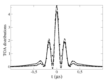
Figure 3: Time-of-arrival distributions: Flux $J$ (dashed line), $\Pi_{K}$ (solid line), $\Pi_{Zeno}$ (big sparse dots), and $\Pi_{chopping}$ (for pulses separated by $\delta t=0.266$ ns, dotted line). The initial wave packet is a combination $\psi=2^{-1/2}(\psi_{1}+\psi_{2})$ of two Gaussian states for the center-of-mass motion of a single Caesium atom that become separately minimal uncertainty packets (with $\Delta x_{1}=\Delta x_{2}=0.021\,\mu$m, and average velocities $\langle v\rangle_{1}=18.96$ cm/s, $\langle v\rangle_{2}=5.42$ cm/s) at $x=0$ and $t=0\,\,\mu$s.

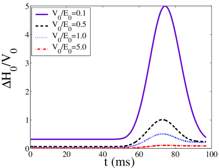
Figure 4: Diminishing ratio $\Delta H_{0}/V_{0}$ with increasing $V_{0}$ versus time for the same initial wave function as in Fig. 2 (²³Na atoms.) $E_{0}$ is the initial kinetic energy.

Figures 2 and 3 illustrate this agreement: in Fig. 2 (inset) the average absorption time, $\langle t\rangle=\int^{\infty}_{0}(-dN/dt)tdt/[1-N(\infty)]$, is shown versus $\delta t$ and $10\hbar/V_{0}$ for a Gaussian wave packet sent from the left towards the origin. The main figure shows the time averages versus $\delta t$ (chopping) and $\hbar/2V_{0}$ (continuous). The lines bend at high coupling because of reflection. The normalized absorption distribution as $V_{0}\to\infty$ was derived in ked05 by making explicit use of the known stationary scattering wave-functions,

$$\Pi_{N}(t)=\frac{\hbar}{mk_{0}}\langle{\psi_{f}(t)}|\widehat{k}\delta(\widehat{x})\widehat{k}|{\psi_{f}(t)}\rangle,$$ (9)

where $k_{0}\hbar$ is the initial average momentum. Fig. 3 shows for a more challenging state, a combination of two Gaussians, that this ideal distribution becomes indistinguable from the normalized chopping distribution when $\delta t$ is small enough. Even the minor details are reproduced, and differ from $J$ and $\Pi_{k}$, also shown.

To understand the compatibility “miracle” of the inequalities (5) and (8), we apply the Robertson-Schrödinger (generalized uncertainty principle) relation,

$$\left|\langle[\widehat{V},\widehat{H}_{0}]\rangle\right|\leq 2|\Delta V_{I}|\Delta H_{0},$$ (10)

where $\Delta$ denotes the standard deviation. Since $|\Delta V_{I}|$ is rigorously bounded at all times by $V_{0}/2$ , imposing $\delta tV_{0}=\alpha\hbar$ with $\alpha\gg 1$, a sufficient condition for dynamical agreement among the models is

$$V_{0}\gg\Delta H_{0}.$$ (11)

For large $V_{0}$ the packet is basically reflected by the wall so that $\Delta H_{0}$ tends to retain its initial value and Eq. (11) will be satisfied during the whole propagation. Fig. 4 shows the ratio $\Delta H_{0}/V_{0}$ for three values of $V_{0}$ as a function of time.

This implies in summary that $\Pi_{Zeno}=\Pi_{N}$, Eq. (9), a very remarkable result, which illustrates that an active intervention on the system dynamics may after all provide an ideal quantity defined for the system in isolation.

III An approximate relation between pulsed and continuous measurements

So far we have discussed the limits $\delta t,\hbar/V_{0}\to 0$ in order to find the corresponding time distribution. In fact a very simple argument relates the pulsed and continuous measurements approximately for finite, non-zero values of $\delta t$ and $\hbar/V_{0}$, when they are sufficiently large to make reflection negligible: the average detection time is delayed with respect to the ideal limit corresponding to $\Pi_{Zeno}$ as

$$\langle t\rangle\approx\langle t\rangle_{Zeno}+\delta t/2\approx\langle t\rangle_{Zeno}+\frac{\hbar}{2V_{0}},$$ (12)

see Fig. 2, since, once a particle is in $x>0$, $\frac{\hbar}{2V_{0}}$ and $\delta t/2$ are precisely the average life times in the continuous and discrete measuring models, respectively . This suggests an approximate agreement between projection and continuous dynamics provided that the relation $\delta t\approx\hbar/V_{0}$ is satisfied. For large $V_{0}$, this is asymptotically not in contradiction with the requirement of a large $\alpha$ since $V_{0}^{-1}-(\alpha V_{0})^{-1}\to 0$ as $V_{0}\to\infty$; in any case quantum reflection breaks down the linear dependence, see Fig. 2.

A similar relation between pulsed and continuous measurements was described by Schulman Schulman98 and has been tested experimentally ket07 . The simplest model in Schulman98 may be reinterpreted as a two-level atom in a resonant laser field, with the excited state decaying away from the 2-level subspace at a rate $\gamma$ mug06 , $\widehat{H}=\frac{\hbar}{2}\left({0\atop\Omega}{\Omega\atop{-i\gamma}}\right)$. The relation between pulsed and continuous measurements follows by comparing the exponential decay for the effective 2-level Hamiltonian with Rabi frequency $\Omega$ and excited state lifetime $1/\gamma$, with the decay dynamics when $\gamma=0$ and the system is projected every $\delta t$ into the ground state. It takes the form Schulman98 $\delta t=\frac{4}{\gamma}$ for $\gamma/\Omega\ll 1$ (weak driving). In our TOA model we have a different set of parameters but a comparison is possible by taking into account that the imaginary potential (4) may be physically interpreted as the effective interaction for the ground state in the weak driving regime, for a localized resonant laser excitation with subsequent decay, $\widehat{H}=\widehat{H}_{0}+\frac{\hbar}{2}\left({0\atop\Omega\Theta(\widehat{x})}{\Omega\Theta(\widehat{x})\atop{-i\gamma}}\right)$. This gives ON03 ; rus04 $V_{0}=\frac{\hbar\Omega^{2}}{2\gamma}$, so that $\delta t\approx\hbar/V_{0}$ becomes

$$\delta t\approx 2\frac{\gamma}{\hbar\Omega^{2}},$$ (13)

different from Schulman’s relation, as it may be expected since the pulsed evolution depends on $\Omega$ in Schulman’s model but not in our case, where it is only driven by the kinetic energy Hamiltonian $\widehat{H}_{0}$.

IV Discussion

The first discussions of the Zeno effect, understood as the hindered passage of the system between orthogonal subspaces because of frequent instantaneous measurements, emphasized its problematic status and regarded it as a failure to simulate or define quantum passage-time distributions. We have shown here that in fact there is a “bright side” of the effect: by normalizing the little bits of norm removed at each projection step, a physical time distribution defined for the freely moving system emerges. (There are other “positive” uses of the Zeno effect, such as reduction of decoherence in quantum computing, see e.g. NTY ; f05 .) In the case of the projection measurements to determine the TOA, this distribution is given by Eq. (9). This result is fundamentally different from the current density or from Kijowski’s TOA distribution, (operational approaches to measure them by fluorescence are described in dam02 ; ON03 ) and corresponds to a classical time-distribution of local kinetic energy density coh79 ; ked05 , rather than a classical TOA distribution .

Experimental realizations of repeated measurements will rely on projections with a finite frequency and pulse duration that provide approximations to the ideal result. Feasible schemes may be based on pulsed localized resonant-laser excitation ket07 , or sweeping with a detuned laser sweep . A challenging open question for further research is the possibility to devise alternative (non periodic) pulse sequences to enhance the robustness of the Zeno effect in a TOA measurement, similar in spirit to the ones proposed in the context of quantum information processing Lidar . Nevertheless, the ordinary (periodic) sequence has successfully been applied in quantum optical realizations of the quantum Zeno effect ket07 .

The proposed normalization method may be applied to other measurements as well, i.e. not only for a TOA of freely moving particles, but in general to first passages between orthogonal subspaces, and it will be interesting to find out in each case the ideal time distribution brought out by normalization.

- (1) J. A. Damborenea, I. L. Egusquiza, G. C. Hegerfeldt, and J. G. Muga, Phys. Rev. A 66, 052104 (2002).
- (2) J. Ruseckas and B. Kaulakys, Phys. Rev. A 66, 052106 (2002).
- (3) D. Alonso, R. S. Mayato, C. R. Leavens, Phys. Rev. A 66, 042108 (2002).
- (4) G. C. Hegerfeldt, D. Seidel, and J. G. Muga, Phys. Rev. A 68, 022111 (2003).
- (5) E.A. Galapon, R.F. Caballar, and R.T. Bahague, Phys. Rev. Lett. 93, 180406 (2004).
- (6) A. Ruschhaupt, J. A. Damborenea, B. Navarro B, J. G. Muga, and G. C. Hegerfeldt, Europhys. Lett. 67, 1 (2004).
- (7) R. S. Bondurant, Phys. Rev. A 69, 062104 (2004).
- (8) E. A. Galapon, F. Delgado, J. G. Muga, and I. Egusquiza, Phys. Rev. A 74, 042107 (2005).
- (9) L. Lamata and J. León, Concepts Phys. 2, 49 (2005).
- (10) Ch. Anastopoulos and N. Savvidou, J. Math. Phys. 47, 122106 (2006).
- (11) G. C. Hegerfeldt, J. T. Neumann, and L. S. Schulman, J. Phys. A 39, 14447 (2006).
- (12) O. del Barco O, M. Ortuño, and V. Gasparian, Phys. Rev. A 74, 032104 (2006).
- (13) G. C. Hegerfeldt, J. T. Neumann, and L. S. Schulman, Phys. Rev. A 75, 012108 (2007).
- (14) M. M Ali, D. Home, A. S. Majumdar, A. K. Pan, Phys. Rev. A 75, 042110 (2007).
- (15) G. Torres-Vega, Phys. Rev. A 75, 032112 (2007).
- (16) A. Gozdz and M. Debicki, Physics of Atomic Nuclei 70, 529 (2007).
- (17) J. G. Muga and C. R. Leavens, Phys. Rep. 338, 353 (2000).
- (18) J. G. Muga, R. Sala and I. L. Egusquiza (eds.), Time in Quantum Mechanics (Springer, Berlin, 2002).
- (19) G. R. Allcock, Ann. Phys. (N.Y.) 53, 253 (1969); 53, 286 (1969); 53, 311 (1969).
- (20) B. Misra and E. C. G. Sudarshan, J. Math. Phys. 18, 756 (1977).
- (21) D. Home and A. Whitaker, Ann. Phys. 258, 237 (1997).
- (22) P. Facchi and S. Pascazio, Prog. in Optics 42, 147 (2001).
- (23) K. Koshino and A. Shimizu, Phys. Rep. 412, 191 (2005).
- (24) P. Facchi, S. Pascazio, A. Scardicchio, and L. S. Schulman, Phys. Rev. A 65, 012108 (2001).
- (25) P. Facchi, G. Marmo, S. Pascazio, A. Scardicchio, and E. C. G. Sudarshan, J. Opt. B: Quantum Semiclass. Opt. 6, S492 (2004).
- (26) P. Exner and T. Ichinose, Ann. Inst. H. Poincaré 6, 195 (2005).
- (27) J. Kijowski, Rep. Math. Phys. 6, 361 (1974).
- (28) F. Delgado, J. G. Muga, and G. García-Calderón, Phys. Rev. A 74, 062102 (2006).
- (29) J. von Neumann, “Mathematical Foundations of Quantum Mechanics”, Princeton University Press, Princeton, 1955.
- (30) L. S. Schulman, Phys. Rev. A 57, 1509 (1998).
- (31) E. W. Streed, J. Mun, M. Boyd, G. K. Campbell, P. Medley, W. Ketterle, and D. E. Pritchard, Phys. Rev. Lett. 97, 260402 (2006).
- (32) H. Nazakato, T. Takazawa, and K. Yuasa, Phys. Rev. Lett. 90, 060401 (2003).
- (33) P. Facchi, S. Tasaki, S. Pascazio, H. Nakazato, A. Tokuse, and D. A. Lidar, Phys. Rev. A 71, 022302 (2005).
- (34) J. G. Muga, D. Seidel, and G. C. Hegerfeldt, J. Chem. Phys. 122, 154106 (2005).
- (35) L. Cohen, J. Chem. Phys. 70, 788 (1979).
- (36) C. S. Chuu, F. Schreck, T. P. Meyrath, J. L. Hanssen, G. N. Price, and M. G. Raizen, Phys. Rev. Lett. 95, 260403 (2005).
- (37) K. Khodjasteh and D. A. Lidar, Phys. Rev. Lett. 95, 180501 (2005).