Effects of Schwarzschild Geometry on Isothermal Plasma Wave Dispersion

The behavior of isothermal plasma waves has been analyzed near the Schwarzschild horizon. We consider a non-rotating background with non-magnetized and magnetized plasmas. The general relativistic magnetohydrodynamical equations for the Schwarzschild planar analogue spacetime with an isothermal state of the plasma are formulated. The perturbed form of these equations is linearized and Fourier analyzed by introducing simple harmonic waves. The determinant of these equations in each case leads to a complex dispersion relation, which gives complex values of the wave number. This has been used to discuss the nature of the waves and their characteristics near the horizon.

PACS numbers: 95.30.Sf, 95.30.Qd, 04.30.Nk

Keywords: 3+1 formalism, GRMHD, Schwarzschild planar analogue, Isothermal plasma

1 INTRODUCTION

General Relativity (GR) is a beautiful scheme for describing the gravitational field. This theory is believed to apply to all forms of interactions, especially between large scale gravitational structures. It has been proven that black holes exist on the basis of study of the effects they exert on their surroundings. They greatly affect the surrounding plasma medium with their enormous gravitational fields. Since all compact objects have strong gravitational fields near their surfaces [1], it is important to study the general relativistic effects on physical processes, like electromagnetic processes taking place in their vicinity. Magnetohydrodynamics (MHD) with the effects of gravity is called general relativistic magnetohydrodynamics (GRMHD). The GRMHD equations help us to study stationary configurations and dynamic evolution of a conducting fluid in a magnetosphere. They include Maxwell’s equations, Ohm’s law and mass, momentum, and energy conservation equations. These equations are required to investigate various aspects of the interaction of relativistic gravity with a plasma’s magnetic field.

The 3+1 formalism is well-suited to carry non-relativistic intuition of physicists about plasmas, hydrodynamics, and stellar dynamics into the arena of black holes and general relativity. This formalism (also called the ADM formalism) was originally developed by Arnowitt et al. [2]. It was motivated by several startling results proved in the 1970s by using a black-hole viewpoint [3-9]. Thorne and Macdonald [10] and Thorne et al. [11] extended this formulation to electromagnetic fields in black-hole theory. The wave propagation theory in Friedmann universe was investigated in a 3+1 formalism by Holcomb and Tajima [12], Holcomb [13], and Dettmann et al. [14]. Khanna [15] derived the MHD equations describing the two-component plasma theory of a Kerr black hole in this split. Komissarov [16] discussed the Blandford-Znajek monopole solution by using the 3+1 formalism in black-hole electrodynamics. Zhang [17,18] formulated the black-hole theory for stationary symmetric GRMHD by using the 3+1 formalism with its applications on a Kerr geometry.

The formalism for gravitational perturbations away from the Schwarzschild background has been developed by Regge and Wheeler [19]. It was extended by Zerilli [20], who showed that the perturbations corresponding to changes in the mass, the angular momentum, and the charge of the Schwarzschild black hole are well-behaved. The decay of non-well-behaved perturbations has been investigated by Price [21]. The quasi-static electric problem was solved by Hanni and Ruffini [5], who proved that the lines of force diverge at the horizon for an observer at infinity. Wald [22] derived the solution for the electromagnetic field occurring when a stationary axisymmetric black hole is placed in a uniform magnetic field aligned along the symmetry axis of the black hole. A linearized treatment of plasma waves for a special relativistic formulation of the Schwarzschild black hole was developed by Sakai and Kawata [23]. Buzzi et al. [24] extended this treatment to waves propagating in the radial direction in a general-relativistic two-component plasma by using the 3+1 ADM formalism. They investigated wave modes for one-dimensional radial propagation of transverse and longitudinal waves close to the Schwarzschild horizon.

The aim of this paper is to investigate the properties of isothermal plasma waves by taking the Schwarzschild spacetime in a planar analogue. The scheme of the paper is as follows: The next section provides comprehensive details about the results in the 3+1 formalism. In Section III, we obtain the GRMHD equations for a perfect fluid with perfect MHD flow conditions. Section IV describes the perturbations and relative assumptions that will be used in the ensuing sections. In Section V, we apply the perturbations and Fourier-analysis methods to the GRMHD equations. Section VI investigates the dispersion relations obtained in graphical forms. The last section contains a summary and discussion of the results.

2 3+1 SPACETIME MODELING

In the $3+1$ formalism, the line element of the spacetime can be written as [18]

$$ds^{2}=-\alpha^{2}dt^{2}+\gamma_{ij}(dx^{i}+\beta^{i}dt)(dx^{j}+\beta^{j}dt),$$ (2.1)

where $\alpha$ is the lapse function, $\beta^{i}$ are components of the shift vector, and $\gamma_{ij}$ are components of the spatial metric. All these quantities are functions of coordinates $t$ and $x^{i}$. A natural observer, associated with this spacetime and called the fiducial observer (FIDO), has a four-velocity n perpendicular to the hypersurfaces of constant time $t$ and is given by

$$\bf{n}=\frac{1}{\alpha}(\frac{\partial}{\partial t}-\beta^{i}\frac{\partial}{\partial x^{i}}).$$

Notice that we are using geometrized units so that $G=1=c$. In four-dimensional spacetime, vectors and tensors will be denoted by boldface italic letters. A letter having a dyad over it will show a three-dimensional tensor. All vector analysis notations, such as gradient, curl and vector product, will be those of the three-dimensional absolute space with the three metric $\overleftrightarrow{\gamma}$. The Latin letters $i,j,k,...$ represent indices in absolute space and run from 1 to 3.

The perfect MHD flow assumption [17] is

$$\textbf{E}+\textbf{V}\times\textbf{B}=0,$$ (2.2)

where V, E, and B are the velocity and the electric and magnetic fields of the fluid as measured by the FIDO. This shows that there can be no electric field in the fluid’s rest-frame.

Applying this condition, Faraday’s law in the 3+1 formalism becomes

$$\frac{d\textbf{B}}{d\tau}+\frac{1}{\alpha}(\textbf{B}.\nabla)\beta+\theta\textbf{B}=\frac{1}{\alpha}\nabla\times(\alpha\textbf{V}\times\textbf{B}),$$ (2.3)

where the FIDO’s four-velocity expansion rate and FIDO’s measured rate of change of any three-dimensional vector in absolute space (i.e., orthogonal to n) can be expressed, respectively, as

$$\theta=\frac{1}{\alpha}(\frac{g_{,t}}{2g}-\nabla.\beta),\quad\frac{d}{d\tau}\equiv\frac{1}{\alpha}(\frac{\partial}{\partial t}-\beta.\nabla).$$

For perfect MHD flow, the equations of evolution of the magnetic field give

$$\frac{D\textbf{B}}{D\tau}+\frac{1}{\alpha}(\textbf{B}.\nabla)(\beta-\alpha\textbf{V})+\left\{\theta+\frac{1}{\alpha}\nabla.(\alpha\textbf{V})\right\}\textbf{B}=0,$$ (2.4)

where

$$\frac{D}{D\tau}\equiv\frac{d}{d\tau}+\textbf{V}.\nabla=\frac{1}{\alpha}\left\{\frac{\partial}{\partial t}+(\alpha\textbf{V}-\beta).\nabla\right\}$$

is the time derivative moving with the fluid. The local conservation law of the rest mass according to the FIDO is

$$\frac{D\rho_{0}}{D\tau}+\rho_{0}\gamma^{2}\textbf{V}.\frac{D\textbf{V}}{D\tau}+\frac{\rho_{0}}{\alpha}\left\{\frac{g_{,t}}{2g}+\nabla.(\alpha\textbf{V}-\beta)\right\}=0,$$ (2.5)

with $\rho_{0}$ being the rest-mass density. The law of force balance measured by the FIDO is given by

$$\left\{\left(\rho_{0}\gamma^{2}\mu+\frac{\textbf{B}^{2}}{4\pi}\right)\gamma_{ij}+\rho_{0}\gamma^{4}\mu V_{i}V_{j}-\frac{1}{4\pi}B_{i}B_{j}\right\}\frac{DV^{j}}{D\tau}+\rho_{0}\gamma^{2}V_{i}\frac{D\mu}{D\tau}$$

$$-\left(\frac{\textbf{B}^{2}}{4\pi}\gamma_{ij}-\frac{1}{4\pi}B_{i}B_{j}\right){V^{j}}_{|k}V^{k}=-\rho_{0}\gamma^{2}\mu\left\{a_{i}-\frac{1}{\alpha}\beta_{j|i}V^{j}-(\pounds_{t}\gamma_{ij})V^{j}\right\}$$

$$-p_{|i}+\frac{1}{4\pi}(\textbf{V}\times\textbf{B})_{i}\nabla.(\textbf{V}\times\textbf{B})-\frac{1}{8\pi\alpha^{2}}(\alpha\textbf{B})^{2}_{|i}+\frac{1}{4\pi\alpha}(\alpha\textbf{B}_{i})_{|j}B^{j}$$

$$-\frac{1}{4\pi\alpha}[\textbf{B}\times\{\textbf{V}\times(\nabla\times(\alpha\textbf{V}\times\textbf{B})-(\textbf{B}.\nabla)\beta)+(\textbf{V}\times\textbf{B}).\nabla\beta\}]_{i},$$ (2.6)

where $p$ is the pressure. The FIDO’s measured local energy conservation law [17] is given by

$$\frac{d\epsilon}{d\tau}+\theta\epsilon+\frac{1}{2\alpha}W^{ij}(\pounds_{t}\gamma^{ij})=-\frac{1}{\alpha^{2}}\nabla.(\alpha^{2}\bf{S})+\frac{1}{\alpha}\nabla\beta:\overleftrightarrow{\bf{W}}+\bf{E}.\bf{j}.$$ (2.7)

When we substitute the following values for a perfect fluid,

$$\epsilon = (\mu\rho_{0}-p(1-\textbf{V}^{2}))\gamma^{2},$$

S $$= \mu\rho_{0}\gamma^{2}\textbf{V},$$

$$\overleftrightarrow{\textbf{W}} = \mu\rho_{0}\gamma^{2}\textbf{V}\otimes\textbf{V}+p\overleftrightarrow{\gamma},$$

with $\mu$ being the specific enthalpy, and perfect MHD flow assumption, Eq. (2.7) becomes

$$\rho_{0}\gamma^{2}\frac{D\mu}{D\tau}+\mu\gamma^{2}\frac{D\rho_{0}}{D\tau}+2\rho_{0}\mu\gamma^{4}\textbf{V}.\frac{D\textbf{V}}{D\tau}-\frac{dp}{d\tau}+(\mu\rho_{0}\gamma^{2}-p)\theta+2\rho_{0}\mu\gamma^{2}\textbf{V}.\textbf{a}$$

$$+\rho_{0}\mu\gamma^{2}(\nabla.\textbf{V})-\frac{1}{\alpha}\{\rho_{0}\mu\gamma^{2}\textbf{V}.(\textbf{V}.\nabla)\beta+p(\nabla.\beta)\}+\frac{1}{2\alpha}\{\rho_{0}\mu\gamma^{2}V^{i}V^{j}$$

$$+p\gamma^{ij}\}\pounds_{t}\gamma_{ij}+\frac{1}{4\pi\alpha}[(\textbf{V}\times\textbf{B}).(\nabla\times(\alpha\textbf{B}))+\theta\alpha(\textbf{V}\times\textbf{B})$$

$$+\alpha(\textbf{V}\times\textbf{B}).\frac{d}{d\tau}(\textbf{V}\times\textbf{B})+(\textbf{V}\times\textbf{B}).(\textbf{V}\times\textbf{B}.\nabla)\beta.(\textbf{V}\times\textbf{B})]=0$$ (2.8)

with acceleration $a=\frac{\nabla\alpha}{\alpha}$. Equations (2.3)-(2) and (2) are the perfect GRMHD equations for a plasma in the vicinity of a black hole.

3 GRMHD EQUATIONS FOR ISOTHERMAL PLASMA IN SCHWARZSCHILD PLANAR ANALOGUE

This section will give a detailed structure of the chosen spacetime with the respective form of the GRMHD equations.

3.1 Description of the Planar Schwarzschild Spacetime and the Equation of State

The planar approximation of the Schwarzschild line element [18] is

$${}ds^{2}=-\alpha^{2}(z)dt^{2}+dx^{2}+dy^{2}+dz^{2},$$ (3.1)

which is an analogue of the Schwarzschild spacetime with $z$, $x$ and $y$ as radial $r$, axial $\phi$, and poloidal $\theta$ directions, respectively. The lapse function vanishes at the horizon, which can be placed at $z=0$, and increases monotonically to unity as $z$ increases from $0$ to $\infty$. The relationship between the universal time $t$ and the FIDO’s time $\tau$ can be expressed by the time lapse $\alpha\equiv\frac{d\tau}{dt}$. The Schwarzschild black hole is non-rotating; hence, there is no shift of coordinates. In this spacetime, the FIDO has a four-velocity equivalent to $\textbf{n}=\frac{1}{\alpha}\frac{\partial}{\partial t}$.

In the hydrodynamic treatment, the plasma is represented as a perfect fluid. In a planar analogue of the Schwarzschild spacetime, we assume that the system of perfect GRMHD equations is enclosed by the isothermal state of a plasma. This state can be expressed by the following equation [17]:

$$\mu=\frac{\rho+p}{\rho_{0}}=constant,$$ (3.2)

which shows that there is no exchange of the heat between the plasma and the magnetic field of fluid.

3.2 Respective GRMHD Equations

For the Schwarzschild planar analogue given in Eq. (3.1), the GRMHD equations Eqs. (2.3)-(2) and (2), in the 3+1 formalism for the isothermal state of a plasma take the form

$$\frac{\partial\textbf{B}}{\partial t}=\nabla\times(\alpha\textbf{V}\times\textbf{B}),$$ (3.3)

$$\frac{\partial\textbf{B}}{\partial t}+(\alpha\textbf{V}.\nabla)\textbf{B}-(\textbf{B}.\nabla)(\alpha\textbf{V})+\textbf{B}\nabla.(\alpha\textbf{V})=0,$$ (3.4)

$$\frac{\partial(\rho+p)}{\partial t}+(\alpha\textbf{V}.\nabla)(\rho+p)+(\rho+p)\gamma^{2}\textbf{V}.\frac{\partial\textbf{V}}{\partial t}$$

$$+(\rho+p)\gamma^{2}\textbf{V}.(\alpha\textbf{V}.\nabla)\textbf{V}+(\rho+p)\nabla.(\alpha\textbf{V})=0,$$ (3.5)

$$\left\{\left((\rho+p)\gamma^{2}+\frac{\textbf{B}^{2}}{4\pi}\right)\delta_{ij}+(\rho+p)\gamma^{4}V_{i}V_{j}-\frac{1}{4\pi}B_{i}B_{j}\right\}\left(\frac{1}{\alpha}\frac{\partial}{\partial t}+\textbf{V}.\nabla\right)V^{j}$$

$$-\left(\frac{\textbf{B}^{2}}{4\pi}\delta_{ij}-\frac{1}{4\pi}B_{i}B_{j}\right)V^{j}_{,k}V^{k}=-(\rho+p)\gamma^{2}a_{i}+\frac{1}{4\pi}\nabla.(\textbf{V}\times\textbf{B})(\textbf{V}\times\textbf{B})_{i}$$

$$-\frac{(\alpha\textbf{B})^{2}_{,i}}{8\pi\alpha^{2}}+\frac{(\alpha B_{i})_{,j}B^{j}}{4\pi\alpha}-\frac{1}{4\pi\alpha}[\textbf{B}\times\{\textbf{V}\times(\nabla\times(\alpha\textbf{V}\times\textbf{B}))\}]_{i}-p_{,i},$$ (3.6)

$$\gamma^{2}(\frac{1}{\alpha}\frac{\partial}{\partial t}+\textbf{V}.\nabla)(\rho+p)+2(\rho+p)\gamma^{4}\textbf{V}.(\frac{1}{\alpha}\frac{\partial}{\partial t}+\textbf{V}.\nabla)\textbf{V}$$

$$+2(\rho+p)\gamma^{2}\textbf{V}.\textbf{a}-\frac{1}{\alpha}\frac{\partial p}{\partial t}+(\rho+p)\gamma^{2}\nabla.\textbf{V}$$

$$+\frac{1}{4\pi\alpha}[(\textbf{V}\times\textbf{B}).(\nabla\times(\alpha\textbf{B}))+\alpha(\textbf{V}\times\textbf{B}).\frac{1}{\alpha}\frac{\partial}{\partial t}(\textbf{V}\times\textbf{B})]=0.$$ (3.7)

Equations (3.3)-(3.2) are the perfect GRMHD equations for an isothermal plasma in the vicinity of a Schwarzschild black hole. In the rest of the paper, we shall analyze these equations by using perturbations and Fourier analysis procedures.

4 RELATIVE ASSUMPTIONS

In this background, the perturbed flow of the fluid is considered to be along the $z$-axis. Thus the FIDO’s measured four-velocity and magnetic field are along the $z$-axis and can be expressed as

$$\textbf{V}=u(z)\textbf{e}_{\textbf{z}},\quad\textbf{B}=B\textbf{e}_{\textbf{z}},$$

where $B$ is a constant quantity. For this velocity, the Lorentz factor $\gamma$ takes the form $\gamma=\frac{1}{\sqrt{1-u^{2}}}.$

The perturbed flow in the magnetosphere shall be characterized by its fluid density $\rho$, pressure $p$, velocity V, and magnetic field B (as measured by the FIDO). The first-order perturbations in the above-mentioned quantities are denoted by $\delta\rho,~{}\delta p,~{}\delta\textbf{V}$, and $\delta\textbf{B}$. Consequently, the perturbed variables will take the following form:

$${}\rho=\rho^{0}+\delta{\rho}=\rho^{0}+\rho\tilde{\rho}, p=p^{0}+\delta{p}=p^{0}+p\tilde{p},$$

$$\textbf{B}=\textbf{B}^{0}+\delta{\textbf{B}}=\textbf{B}^{0}+B\textbf{b}, \textbf{V}=\textbf{V}^{0}+\delta{\textbf{V}}=\textbf{V}^{0}+\textbf{v},$$ (4.1)

where $\rho^{0},~{}p^{0},~{}\textbf{B}^{0}$ and $\textbf{V}^{0}$ are unperturbed quantities. Due to gravitation, the waves can propagate in the $z$-direction with respect to time $t$. Hence, the perturbed quantities depend on $z$ and $t$.

The following notations for the perturbed quantities will be used:

$$\tilde{\rho}\equiv\frac{\delta\rho}{\rho}=\tilde{\rho}(t,z), \tilde{p}\equiv\frac{\delta p}{p}=\tilde{p}(t,z),$$

$$\textbf{v}\equiv\delta\textbf{V}=v_{z}(t,z)\textbf{e}_{\textbf{z}}, \textbf{b}\equiv\frac{\delta\textbf{B}}{B}=b_{z}(t,z)\textbf{e}_{\textbf{z}}.$$

We also assume that the perturbations have harmonic space and time dependences, i.e.,

$$\tilde{\rho},~{}\tilde{p},~{}\textbf{v}~{}\rm{and}~{}\textbf{b}\sim\it{e^{-i(\omega t-kz)}}.$$

Thus, the perturbed variables can be expressed as

$$\tilde{\rho}(t,z)=c_{1}e^{-\iota(\omega t-kz)},$$

$$\tilde{p}(t,z)=c_{2}e^{-\iota(\omega t-kz)},$$

$$v_{z}(t,z)=c_{3}e^{-\iota(\omega t-kz)},$$

$$b_{z}(t,z)=c_{4}e^{-\iota(\omega t-kz)}.$$ (4.2)

5 PERTURBATION EQUATIONS

If the perturbations given by Eq. (4) are introduced, the GRMHD equations, Eqs. (3.3)-(3.2), become

$$\frac{\partial(\delta\textbf{B})}{\partial t}=\nabla\times(\alpha\textbf{v}\times\textbf{B})+\nabla\times(\alpha\textbf{V}\times\delta\textbf{B}),$$ (5.1)

$$\nabla.(\delta\textbf{B})=0,$$ (5.2)

$$\frac{\partial(\delta\rho+\delta p)}{\partial t}+(\alpha\textbf{V}.\nabla)(\delta\rho+\delta p)+(\rho+p)\gamma^{2}\textbf{V}.\frac{\partial\textbf{v}}{\partial t}-\alpha(\rho+p)\textbf{v}.\nabla\ln u$$

$$+\alpha(\rho+p)(\nabla.\textbf{v})+(\delta\rho+\delta p)\nabla.(\alpha\textbf{V})+(\delta\rho+\delta p)\gamma^{2}\textbf{V}.(\alpha\textbf{V}.\nabla)\textbf{V}$$

$$+2(\rho+p)\gamma^{2}(\textbf{V}.\textbf{v})(\alpha\textbf{V}.\nabla)\ln\gamma+(\rho+p)\gamma^{2}(\alpha\textbf{V}.\nabla\textbf{V}).\textbf{v}$$

$$+(\rho+p)\gamma^{2}\textbf{V}.(\alpha\textbf{V}.\nabla)\textbf{v}=0,$$ (5.3)

$$\{((\rho+p)\gamma^{2}+\frac{\textbf{B}^{2}}{4\pi})\delta_{ij}+(\rho+p)\gamma^{4}V_{i}V_{j}-\frac{1}{4\pi}B_{i}B_{j}\}\frac{1}{\alpha}\frac{\partial v^{j}}{\partial t}$$

$$+\frac{1}{4\pi}[\textbf{B}\times\{\textbf{V}\times\frac{1}{\alpha}\frac{\partial(\delta\textbf{B})}{\partial t}\}]_{i}+(\rho+p)\gamma^{2}v_{i,j}V^{j}+(\rho+p)\gamma^{4}V_{i}v_{j,k}V^{j}V^{k}$$

$$-\frac{1}{4\pi\alpha}\{(\alpha\delta B_{i})_{,j}-(\alpha\delta B_{j})_{,i}\}B^{j}=-\gamma^{2}\{(\delta\rho+\delta p)+2(\rho+p)\gamma^{2}(\textbf{V}.\textbf{v})\}a_{i}$$

$$-(\delta p)_{,i}+\frac{1}{4\pi\alpha}\{(\alpha B_{i})_{,j}-(\alpha B_{j})_{,i}\}\delta B^{j}-(\rho+p)\gamma^{4}(v_{i}V^{j}+v^{j}V_{i})V_{k,j}V^{k}$$

$$-\gamma^{2}\{(\delta\rho+\delta p)V^{j}+2(\rho+p)\gamma^{2}(\textbf{V}.\textbf{v})V^{j}+(\rho+p)v^{j}\}V_{i,j}$$

$$-\gamma^{4}V_{i}\{(\delta\rho+\delta p)V^{j}+4(\rho+p)\gamma^{2}(\textbf{V}.\textbf{v})V^{j}+(\rho+p)v^{j}\}V_{j,k}V^{k},$$ (5.4)

$$\gamma^{2}\frac{1}{\alpha}\frac{\partial(\delta\rho+\delta p)}{\partial t}+\frac{2}{\alpha}(\rho+p)\gamma^{4}\textbf{V}.\frac{\partial\textbf{v}}{\partial t}-2(\rho+p)\gamma^{4}(\textbf{V}.\textbf{v})(\textbf{V}.\nabla)\ln u$$

$$+6(\rho+p)\gamma^{6}(\textbf{V}.\textbf{v})\{\textbf{V}.(\textbf{V}.\nabla)\textbf{V}\}+(\rho+p)\gamma^{4}\textbf{V}.(\textbf{v}.\nabla)\textbf{V}$$

$$+2(\rho+p)\gamma^{4}\textbf{V}.(\textbf{V}.\nabla)\textbf{v}+2(\delta\rho+\delta p)\gamma^{2}\textbf{V}.\textbf{a}+2(\rho+p)\gamma^{4}(\textbf{V}.\textbf{v})(\textbf{V}.\textbf{a})$$

$$+(\rho+p)\gamma^{2}(\nabla.\textbf{v})+(\rho+p)\gamma^{2}\textbf{v}.\textbf{a}+\gamma^{2}(\textbf{V}.\nabla)(\delta\rho+\delta p)-\frac{1}{\alpha}\frac{\partial(\delta p)}{\partial t}$$

$$-(\rho+p)\gamma^{2}(\textbf{v}.\nabla)\ln u+2(\delta\rho+\delta p)\gamma^{4}\textbf{V}.(\textbf{V}.\nabla)\textbf{V}+(\delta\rho+\delta p)\gamma^{2}(\nabla.\textbf{V})$$

$$+2(\rho+p)\gamma^{4}(\textbf{V}.\textbf{v})(\nabla.\textbf{V})+2(\rho+p)\gamma^{4}\textbf{v}.(\textbf{V}.\nabla)\textbf{V}+\frac{1}{4\pi\alpha}[(\textbf{V}\times\textbf{B}).$$

$$(\nabla\times(\alpha\delta\textbf{B}))+(\textbf{v}\times\textbf{B}).(\nabla\times(\alpha\textbf{B}))+(\textbf{V}\times\delta\textbf{B}).(\nabla\times(\alpha\textbf{B}))$$

$$+(\textbf{V}\times\textbf{B}).(\textbf{V}\times\frac{\partial\delta\textbf{B}}{\partial t})+(\textbf{V}\times\textbf{B}).(\frac{\partial\textbf{v}}{\partial t}\times\textbf{B})]=0.$$ (5.5)

The component forms of Eqs. (LABEL:c2)-(5) are given as

$$\frac{1}{\alpha}\frac{\partial b_{z}}{\partial t}=0,$$ (5.6)

$$b_{z,z}=0,$$ (5.7)

$$\rho\frac{\partial\tilde{\rho}}{\partial t}+u\alpha(\rho\tilde{\rho}_{,z}+p\tilde{p}_{,z})+p\frac{\partial\tilde{p}}{\partial t}+\gamma^{2}u(\rho+p)\frac{\partial v_{z}}{\partial t}$$

$$+\alpha(\rho+p)(1+\gamma^{2}u^{2})v_{z,z}-(\tilde{\rho}-\tilde{p})\{(\alpha up)^{\prime}+\alpha\gamma^{2}u^{2}pu^{\prime}\}$$

$$=\alpha(\rho+p)(1-2\gamma^{2}u^{2})(1+\gamma^{2}u^{2})\frac{u^{\prime}}{u}v_{z},$$ (5.8)

$$(\rho+p)\gamma^{2}(1+\gamma^{2}u^{2})\left\{\frac{1}{\alpha}\frac{\partial v_{z}}{\partial t}+uv_{z,z}\right\}+p\tilde{p}_{,z}+\tilde{p}p_{,z}$$

$$=-\gamma^{2}(\rho+p)\{u^{\prime}(1+\gamma^{2}u^{2})(1+4\gamma^{2}u^{2})+2u\gamma^{2}a_{z})\}v_{z}$$

$$-(\rho\tilde{\rho}+p\tilde{p})\gamma^{2}\{a_{z}+u(1+\gamma^{2}u^{2})u^{\prime}\},$$ (5.9)

$$\rho\gamma^{2}\frac{1}{\alpha}\frac{\partial}{\partial t}\tilde{\rho}+p\gamma^{2}\frac{1}{\alpha}\frac{\partial}{\partial t}\tilde{p}+\frac{2}{\alpha}(\rho+p)\gamma^{4}u\frac{\partial v_{z}}{\partial t}+(\rho+p)\gamma^{2}(1+2\gamma^{2}u^{2})v_{z,z}$$

$$+(\rho\tilde{\rho}+p\tilde{p})\gamma^{2}\{2ua_{z}+(1+2\gamma^{2}u^{2})u^{\prime}\}+\gamma^{2}u(\rho_{,z}\tilde{\rho}+\tilde{\rho}_{,z}\rho+p_{,z}\tilde{p}+\tilde{p}_{,z}p)$$

$$-p\frac{1}{\alpha}\frac{\partial\tilde{p}}{\partial t}+(\rho+p)\gamma^{2}\left\{(3\gamma^{2}uu^{\prime}+a_{z})(1+2\gamma^{2}u^{2})-\frac{u^{\prime}}{u}\right\}v_{z}=0.$$ (5.10)

The conservation law of rest-mass [17] in a three-dimensional hypersurface for the isothermal state of a plasma,

$$\alpha(\rho+p)\gamma u=constant,$$

is used to obtain Eqs. (5) and (5). The same law will be applied for further simplifications.

Using Eq. (4) in Eqs. (5.6)-(5), we obtain the Fourier-analyzed form of the above equations as

$$-\frac{\iota\omega}{\alpha}c_{4}=0,$$ (5.11)

$$\iota kc_{4}=0,$$ (5.12)

$$c_{1}\{-\rho\iota\omega+\iota k\rho\alpha u-(u\alpha p)^{\prime}-\alpha u^{2}\gamma^{2}pu^{\prime}\}+c_{2}\{-p\iota\omega+\iota kp\alpha u$$

$$+(u\alpha p)^{\prime}+\alpha u^{2}\gamma^{2}pu^{\prime}\}+c_{3}(\rho+p)\left\{\alpha(1+\gamma^{2}u^{2})\iota k\right.$$

$$\left.-\alpha(1-2\gamma^{2}u^{2})(1+\gamma^{2}u^{2})\frac{u^{\prime}}{u}-i\omega\gamma^{2}u\right\}=0,$$ (5.13)

$$c_{1}\rho\gamma^{2}\{a_{z}+uu^{\prime}(1+\gamma^{2}u^{2})\}+c_{2}\{p\gamma^{2}\{a_{z}+uu^{\prime}(1+\gamma^{2}u^{2})\}+\iota kp+p^{\prime}\}$$

$$+c_{3}(\rho+p)\gamma^{2}\left[(1+\gamma^{2}u^{2})\left(\frac{-\iota\omega}{\alpha}+\iota uk\right)+\{u^{\prime}(1+\gamma^{2}u^{2})(1+4\gamma^{2}u^{2})\right.$$

$$\left.+2ua_{z}\}\right]=0,$$ (5.14)

$$\left\{\rho\gamma^{2}\left(\frac{-\iota\omega}{\alpha}+\iota ku\right)+\gamma^{2}u\rho^{\prime}+\rho 2\gamma^{2}ua_{z}+\rho(1+2\gamma^{2}u^{2})\gamma^{2}u^{\prime}\right\}c_{1}$$

$$+\left\{\frac{-\iota\omega}{\alpha}p(\gamma^{2}-1)+\iota k\gamma^{2}up+\gamma^{2}up^{\prime}+2\gamma^{2}upa_{z}+p(1+2\gamma^{2}u^{2})\gamma^{2}u^{\prime}\right\}c_{2}$$

$$+(\rho+p)\gamma^{2}\left\{\frac{-2\iota\omega}{\alpha}\gamma^{2}u+\iota k(1+2\gamma^{2}u^{2})+3\gamma^{2}uu^{\prime}(1+2\gamma^{2}u^{2})\right.$$

$$\left.+a_{z}(1+2\gamma^{2}u^{2})-\frac{u^{\prime}}{u}\right\}c_{3}=0.$$ (5.15)

Equations (5.11) and (5.12) yield that $c_{4}=0$; i.e., the magnetic field is not affected by the black-hole gravity and time. It is mentioned here that Eqs. (5)-(5) also give a non-magnetized plasma.

6 NUMERICAL SOLUTIONS

We consider that the magnetosphere is filled with a stiff fluid for which $\rho=constant=p$ and let $\alpha=\tanh(z)$. Using these values, the mass conservation law in 3-dimensions gives $u=\frac{1}{\sqrt{1+\tanh^{2}(z)}}$.

When we use these values, the determinant of the coefficients of constants $c_{1},~{}c_{2}$, and $c_{3}$ in Eqs. (5)-(5) give a complex dispersion equation of the type

$$A_{1}(z)k^{2}+A_{2}(z,\omega)k+A_{3}(z,\omega)+\iota\{A_{4}(z)k^{3}$$

$$+A_{5}(z,\omega)k^{2}+A_{6}(z,\omega)+A_{7}(z,\omega)k\}=0,$$ (6.1)

which, on solving, gives three complex values of $k=k_{1}+\iota k_{2}$. The sinusoidal expressions then take the form $e^{-\iota(\omega t-k_{1}z-\iota k_{2}z)}=e^{-\iota(\omega t-k_{1}z)-k_{2}z}$. It is obvious that $Re(k)$ is the propagation factor and $Im(k)$ is the attenuation factor for a time harmonic plane wave with fixed angular frequency $\omega$ in a dispersive material. Using the values of $k$, the phase velocity ($v_{p}=\frac{\omega}{k_{1}}$) and the group velocity ($v_{g}=\frac{d\omega}{dk_{1}}$) [25] of the waves can be calculated. The three values of the dispersion relation are shown in Figs. 1, 2 and 3.

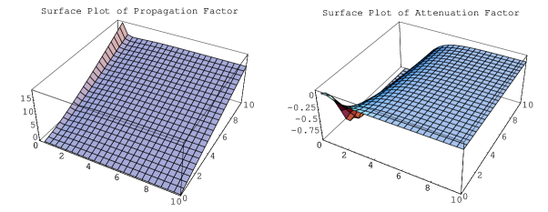
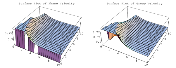
Figure 1: Waves propagate more near the event horizon. They damp as they move away from the event horizon. Anomalous dispersion is found in that region.

Fig. 1 shows that the propagation factor is infinite at the horizon, which indicates that no wave exists there. This has greater value near the event horizon and decreases as we go away from the horizon. It also increases with increasing angular frequency of the wave. The attenuation factor increases, which shows that the waves damp with increasing angular frequency and value of $z$. The phase velocity is greater than the group velocity, which shows that dispersion is normal in the region. The waves with negligible angular frequency have phase velocities less than the group velocities and hence, the medium shows anomalous dispersion.

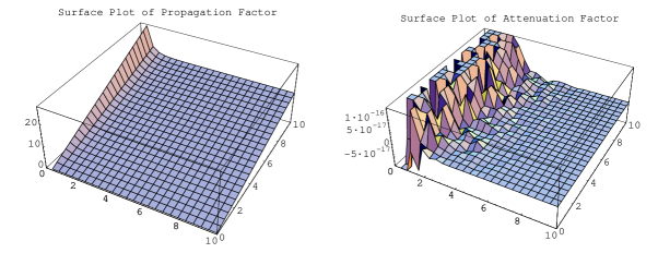
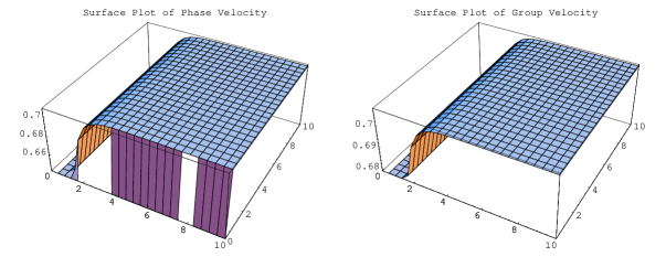
Figure 2: Waves propagate rapidly as they move near the event horizon. The dispersion of waves is anomalous in that region.

The propagation factor in Fig. 2 shows the same behavior as that in Fig. 1. In the region, the attenuation factor takes very small values, which are positive and negative randomly. The phase and the group velocities are the same in the region, except for zero angular frequency waves. For those waves, the phase velocity is less than the group velocity, indicating anomalous dispersion.

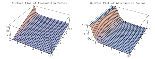
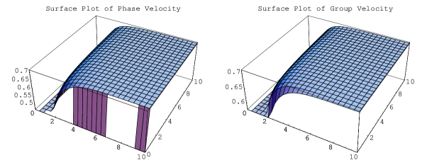
Figure 3: Propagation of waves is more near the event horizon. The waves grow as they move away from the event horizon. The dispersion is found to be anomalous.

In Fig. 3, the propagation factor is greater near the event horizon and decreases as we go away from the horizon, but becomes infinite at the event horizon. The attenuation factor increases when the angular frequency increases and decreases when the value of $z$ increases. The waves grow as they go far from the event horizon of the black hole. Damping occurs when the angular frequency increases. The group velocity of the waves is greater than the phase velocity, which shows anomalous dispersion.

7 SUMMARY

This paper is devoted to discussing the isothermal plasma wave properties of the Schwarzschild black-hole’s magnetosphere by using the 3+1 formalism. For this purpose, the GRMHD equations are derived and discussed by taking one-dimensional perturbations in perfect MHD flow with its planar analogue. These equations are written in component form and then Fourier analyzed by using the assumption of plane waves. We have assumed that the black hole’s gravity does not introduce any effect on magnetic field. The determinant of the coefficients are solved to get complex dispersion relations, which yield the wave numbers. The properties of plasma are inferred on the basis of this number, and the relevant quantities are obtained in graphical form. A summary of the results is given below:

From the three dispersion relations, we find that the wave propagation factor becomes infinite. This implies that the wave number is infinite at the event horizon; hence, waves vanish there. This corresponds to the well-known fact that no information can be extracted from a black hole.

The attenuation factor assumes extreme values near the event horizon. These values gradually decrease or increase as they move away from the horizon. The gravity of the black hole causes the attenuation factor to take extreme values. Thus, the wave growth or damping is larger near the event horizon. The attenuation factor is indefinite at the event horizon. The wave propagation factor is high near the black hole’s event horizon. As the waves go far from the event horizon, the propagation decreases, which shows that the perturbations are high near the gravitational well.

It is worthwhile mentioning here that waves are highly excited near the event horizon (Fig. 1). This excitement decreases as they move away from the event horizon. This is due to immense gravity of the black hole near the event horizon. Similar is the case of Fig. 2, where the waves are randomly excited near the event horizon.

We notice that the dispersion is anomalous here while for a cold plasma (Fig. 2) [26], normal wave dispersion was found. This indicates that the plasma pressure causes the waves to pass through the region in the neighborhood of the event horizon.

The dispersion relations are obtained by using the 3+1 ADM formalism and contain the factor of acceleration (depends on the lapse function and is equal to $-g$), which makes them different from the usual MHD dispersion relations. We have investigated the waves propagating in a plasma influenced by the gravitational field. We observe that the values of $k$ show gravitational effects on the smooth harmonic wave type perturbations. It would be interesting to investigate the plasma wave properties by taking a rotating background.

ACKNOWLEDGMENT

We appreciate the Higher Education Commission, Islamabad, Pakistan, for its financial support during this work through the Indigenous PhD 5000 Fellowship Program Batch-II.

References

• [1] J. A. Petterson: Phys. Rev. D10, 3166(1974).
• [2] R. Arnowitt, S. Deser, and C. W. Misner: Gravitation: An Introduction to Current Research (Wiley, New York, 1962).
• [3] S. W. Hawking: Nature 248, 30(1974); Commun. Math. Phys. 43, 199(1975); Phys. Rev. D13, 191(1976).
• [4] J. B. Hartle: Phys. Rev. D8, 1010(1973); ibid. 9, 2749(1974).
• [5] R. S. Hanni and R. Ruffini: Phys. Rev. D8, 3259(1973).
• [6] P. Hajicek: Commun. Math. Phys. 36, 305(1974).
• [7] R.L. Znajek: Ph.D. Thesis (University of Cambridge, 1976); Mon. Not. R. Astr. Soc. 185, 833(1978).
• [8] T. Damour: Phys. Rev. D18, 3598(1978); Procs. of Second Marcel Grossman Meeting on General Relativity ed. R. Ruffini, North Holland, Amsterdam, 587(1982).
• [9] T. Damour: Ph.D. Thesis (University of Paris VI, 1979)
• [10] K. S. Thorne and D. A. Macdonald: Mon. Not. R. Astron. Soc. 198, 339(1982); ibid 198, 345(1982).
• [11] K. S. Thorne, R. H. Price and D. A. Macdonald: Black Holes: The Membrane Paradigm (Yale University Press, New Haven, 1986).
• [12] K. A. Holcomb and T. Tajima: Phys. Rev. D40, 3809(1989).
• [13] K. A. Holcomb: Astrophys. J. 362, 381(1990).
• [14] C. P. Dettmann, N. E. Frankel and V. Kowalenko: Phys. Rev. D48, 5655(1993).
• [15] R. Khanna: Mon. Not. R. Astron. Soc. 294, 673(1998).
• [16] S. S. Komissarov: Mon. Not. R. Astron. Soc. 336,759(2002).
• [17] X. -H. Zhang: Phys. Rev. D39, 2933(1989).
• [18] X. -H. Zhang: Phys. Rev. D40, 3858(1989).
• [19] T. Regge and J. A. Wheeler: Phys. Rev. 108, 1063(1957).
• [20] F. Zerilli: Phys.Rev. D2, 2141(1970); J. Math. Phys. 11, 2203(1970); Phys. Rev. Lett. 24, 737(1970).
• [21] R. H. Price: Phys. Rev. D5, 2419(1972); ibid 5, 2439(1972).
• [22] R. M. Wald: Phys. Rev. D10, 1680(1974).
• [23] J. Sakai and T. Kawata: J. Phys. Soc. Jpn. 49, 747(1980).
• [24] V. Buzzi, K. C. Hines and R. A. Treumann: Phys. Rev. D51,6663(1995); ibid 51, 6677(1995).
• [25] K. E. Oughstun and N. A. Cartwright: J. Opt. A: Pure Appl. Opt. 4, S125(2002).
• [26] M. Sharif and U. Sheikh: Complex wave numbers in the vicinity of the Schwarzschild Event Horizon, Int. J. Mod. Phys. A (2007, to appear).