Complex Wave Numbers in the Vicinity of the Schwarzschild Event Horizon

Abstract

This paper is devoted to investigate the cold plasma wave properties outside the event horizon of the Schwarzschild planar analogue. The dispersion relations are obtained from the corresponding Fourier analyzed equations for non-rotating and rotating, non-magnetized and magnetized backgrounds. These dispersion relations provide complex wave numbers. The wave numbers are shown in graphs to discuss the nature and behavior of waves and the properties of plasma lying in the vicinity of the Schwarzschild event horizon.

Keywords : Schwarzschild planar analogue, cold plasma.

1 Introduction

General Relativity is the geometric theory of gravity which deals with four- dimensional spacetime. According to this theory, gravity severely modifies space and time near the black hole. The Schwarzschild black hole, a minimum configuration of the Kerr black hole, exhibits a strong gravitational field [1]. This field pulls the plasma surrounding the black hole event horizon towards and then into the black hole. The plasma is drawn equally from all directions and thus form an omni-directional accretion disk. The existence of this disk is one of the observational facts used to identify a black hole. The motion of plasma inside the accretion disk is governed by the theory of general relativistic magnetohydrodynamics (GRMHD). Maxwell’s equations, Ohm’s law, mass, momentum and energy conservation equations constitute this theory that are required to investigate various aspects of the interaction of relativistic gravity with plasma’s magnetic field.

The theory of general relativity is a sterile subject until it touches the real physical world. Only the hard reality of experiments and of astronomical observations can bring the theory to life. The 3+1 ADM formalism, developed to study the quantization of gravitational field by Arnowitt et al. [2], has mostly been used in numerical relativity [3]-[7]. The 3+1 spacetime split in the formulation of general relativity is particularly appropriate for applications to the black hole theory as described by Thorne et al. [8]-[10]. Wave properties in the Friedmann universe were investigated [11]-[13] by the same formalism. Sakai and Kawata [14] developed a linearized treatment of relativistic plasma waves in analogy with the special relativistic formulation. Khanna [15] derived Ohm’s law for two component plasma theory of the Kerr black hole. Zhang [16]-[17] formulated stationary symmetric GRMHD theory with its applications in Kerr geometry. Buzzi et al. [18]-[19] treated the wave propagation in radial direction close to the Schwarzschild horizon in general relativistic two component plasma.

In a recent paper, Sharif and Umber [20] have investigated real wave numbers and properties of the medium existing in the vicinity of a Schwarz-schild black hole using the same split. The cold plasma is considered in non-rotating or rotating, non-magnetized or magnetized backgrounds. The same authors have also worked out the wave properties in isothermal plasma for the Schwarzschild spacetime planar analogue using ADM split [21]-[22]. It is verified that no information can be extracted either from the event horizon or its exterior.

In this paper, we focus our attention to investigate the wave numbers and properties of the medium for the Schwarzschild planar analogue spacetime. The paper is organized as follows. Section 2 describes the general line element and its specified form (the planar analogue) for the Schwarzschild black hole in 3+1 formalism. It also contains background assumptions. In sections 3, 4 and 5, the dispersion relations for non-rotating (non-magnetized and magnetized), rotating non-magnetized and rotating magnetized backgrounds are investigated respectively. Finally, section 6 provides the outlook of the results.

2 3+1 Spacetime Modeling

The general line element in $3+1$ formalism can be expressed as [17]

$$ds^{2}=-\alpha^{2}dt^{2}+\gamma_{ij}(dx^{i}+\beta^{i}dt)(dx^{j}+\beta^{j}dt),$$

where $\alpha$ is the lapse function, $\beta^{i}$ are the components of the shift vector and $\gamma_{ij}$ are the components of the spatial metric. All these quantities are functions of coordinates $t$ and $x^{i}$. A natural observer, associated with this spacetime called fiducial observer (FIDO), has four-velocity perpendicular to the hypersurfaces of constant time $t$. The planar analogue of the Schwarzschild line element [17] is

$${}ds^{2}=-\alpha^{2}(z)dt^{2}+dx^{2}+dy^{2}+dz^{2},$$ (2.1)

where $z$, $x$ and $y$ are analogues of radial $r$, $\phi$ and $\theta$ directions respectively. The lapse function vanishes at the event horizon placed at $z=0$, and increases monotonically to unity as $z$ increases from $0$ to $\infty$.

2.1 Background Assumptions

We consider two backgrounds with the specifications given below:

1. Non-Rotating Background

   In this background, the fluid flow as well as the external magnetic field lines are along $z$-direction (analogous to the radial direction) moving towards the black hole event horizon. The fluid velocity and the magnetic field lines are taken to be $\textbf{V}=u(z)\textbf{e}_{\textbf{z}}$ and $\textbf{B}=B\textbf{e}_{\textbf{z}}$ respectively.

2. Rotating Background

   This background demands the fluid to move in more than one dimension. Thus we assume that the fluid motion and the external magnetic field according to FIDO as $\textbf{V}=V(z)\textbf{e}_{\textbf{x}}+u(z)\textbf{e}_{\textbf{z}}$ and $\textbf{B}=\lambda(z)B\textbf{e}_{\textbf{x}}+B\textbf{e}_{\textbf{z}}$ respectively, where $B$ is a constant.

In MHD theory, plasma is treated to be a perfect fluid. We assume cold plasma surrounding the Schwarzschild black hole with equation of state

$$\mu=\frac{\rho}{\rho_{0}}=constant$$ (2.2)

which has vanishing thermal pressure and thermal energy. Here $\rho$ is the mass density of the fluid. The fluid flow is assumed to be perturbed by the gravitational field of the black hole. The linearized perturbed quantities take the form

$$\rho=\rho^{0}+\rho\tilde{\rho},\quad\textbf{V}=\textbf{V}^{0}+\textbf{v},\quad\textbf{B}=\textbf{B}^{0}+B\textbf{b}.$$ (2.3)

The variables with superscript zero are unperturbed quantities. The dimensionless notations for the perturbed quantities are

$$\tilde{\rho}=\tilde{\rho}(t,z),\quad\textbf{v}=v_{z}(t,z)\textbf{e}_{\textbf{z}},\quad\textbf{b}=b_{z}(t,z)\textbf{e}_{\textbf{z}}$$ (2.4)

for non-rotating background whereas for rotating background

$$\textbf{v}=v_{x}(t,z)\textbf{e}_{\textbf{x}}+v_{z}(t,z)\textbf{e}_{\textbf{z}},\quad\textbf{b}=b_{x}(t,z)\textbf{e}_{\textbf{x}}+b_{z}(t,z)\textbf{e}_{\textbf{z}}.$$ (2.5)

We assume that the perturbed quantities have harmonic space and time dependence and hence these quantities can be expressed as follows

$$\tilde{\rho}(t,z)=c_{1}e^{-\iota(\omega t-kz)},\quad v_{z}(t,z)=c_{2}e^{-\iota(\omega t-kz)},\quad v_{x}(t,z)=c_{3}e^{-\iota(\omega t-kz)},$$

$$b_{x}(t,z)=c_{4}e^{-\iota(\omega t-kz)},\quad b_{z}(t,z)=c_{5}e^{-\iota(\omega t-kz)}$$ (2.6)

where $c_{1},~{}c_{2},~{}c_{3},~{}c_{4}$ and $c_{5}$ are arbitrary constants, $k$ is the wave number and $\omega$ is the angular frequency of waves.

3 Non-Rotating Background

For the fluid flow in only one dimension, i.e., $z$-direction, we shall use the same Fourier analysed equations given in [20] as follows

$$-\frac{\iota\omega}{\alpha}c_{5}=0,$$ (3.1)

$$\iota kc_{5}=0,$$ (3.2)

$$c_{1}\left(\frac{-\iota\omega}{\alpha}+\iota ku\right)+c_{2}\left\{(1+\gamma^{2}u^{2})\iota k-(1-2\gamma^{2}u^{2})\right.$$

$$\left.\times(1+\gamma^{2}u^{2})\frac{u^{\prime}}{u}-\frac{i\omega}{\alpha}\gamma^{2}u\right\}=0,$$ (3.3)

$$c_{1}\gamma^{2}\{a_{z}+uu^{\prime}(1+\gamma^{2}u^{2})\}+c_{2}[\gamma^{2}(1+\gamma^{2}u^{2})\left(\frac{-\iota\omega}{\alpha}+\iota uk\right)+$$

$$+\gamma^{2}\{u^{\prime}(1+\gamma^{2}u^{2})(1+4\gamma^{2}u^{2})+2u\gamma^{2}a_{z}\}]=0.$$ (3.4)

Equations (LABEL:p1) and (3.2) imply that $c_{5}=0$ which means that no perturbations occur in magnetic field of the fluid. Thus we are left with Eqs.(3) and (3). It is mentioned here that for non-magnetized plasma, we also obtain the same two equations.

3.1 Numerical Solutions

We consider cold plasma of constant density. The time lapse is assumed to be $\tanh(z)$ which vanishes at the horizon $z=0$ and increases to $1$ as $z\rightarrow\infty.$ Using mass conservation law in three dimensions, i.e., $\rho\gamma u=constant$ we obtain the value of $u=\frac{1}{\sqrt{1+\tanh^{2}(z)}}$. The determinant of the coefficients of the constants $c_{1}$ and $c_{2}$ in Eqs.(3) and (3) is a complex number. Solving this determinant by using the software Mathematica, we obtain two complex values of the wave number $k$. Real and imaginary parts of this wave number show the propagation factor and the attenuation factor respectively for plane wave in dispersive medium. The propagation factor gives the phase velocity ($v_{p}=\frac{\omega}{Re(k)}$) and group velocity ($v_{g}=\frac{d\omega}{d(Re(k))}$) of the waves. The sinusoidal expressions then take the form $e^{-\iota(\omega t-k_{1}z-\iota k_{2}z)}=e^{-\iota(\omega t-k_{1}z)-k_{2}z}$, where $k_{1}=Re(k)$ and $k_{2}=Im(k)$. The wave numbers obtained are shown in Figures 1 and 2.

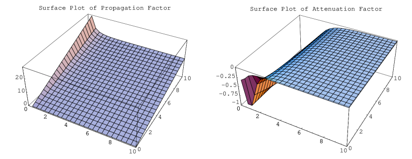
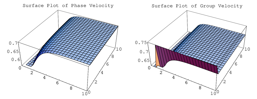
Figure 1: Wave propagation increases near the event horizon. Dispersion is found to be anomalous.

In Figure 1, the waves vanish in the region $0\leq z<1.1\times 10^{-8}$ due to infinite wave number. The propagation factor of the waves is positive for the region $0\leq z<1.1\times 10^{-8},~{}0<\omega\leq 10$. It increases with the increase in angular frequency and decreases with an increase in $z$. Thus the waves propagate rapidly far from the event horizon. The waves with higher angular frequencies move faster than the waves with lower angular frequencies. The attenuation factor increases with an increase in $z$. The waves damp as they move away from the event horizon. The phase velocity is less than the group velocity in the region $0<z\leq 10$ which implies anomalous dispersion of the waves in this region [23]. There is an exceptional case of the waves with very small angular frequency that do not show this behavior.

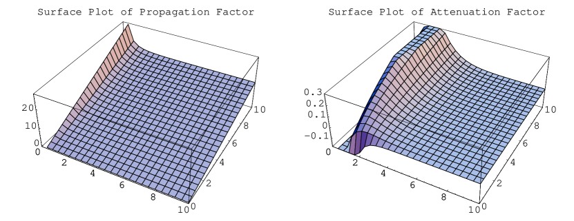
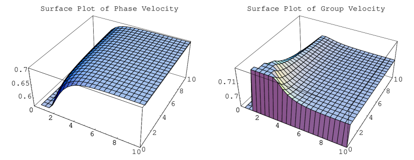
Figure 2: The waves propagate rapidly near the event horizon. The whole region admits normal dispersion.

Figure 2 shows that the wave number is infinite in the region $0\leq z<1.1\times 10^{-8}$. The propagation factor takes negative values in $1.1\times 10^{-8}\leq z\leq 10,~{}0\leq\omega<1\times 10^{-19}$ which shows the same behavior as given in Figure 1 except for this small region. The attenuation factor is negative in the region $1.1\times 10^{-8}\leq z\leq 0.68$ and takes larger values at $z=1.4$ where the waves damp. The waves grow as the angular frequency decreases. The group velocity is less than the phase velocity for the region $0<\omega\leq 10$ which shows normal dispersion of waves.

4 Rotating Non-Magnetized Background

For the rotating background, the Fourier analysed Eqs.(4.13)-(4.15) of [20] are

$$c_{1}\iota\left(-\frac{\omega}{\alpha}+ku\right)+c_{2}\left[-\frac{\iota\omega}{\alpha}\gamma^{2}u+(1+\gamma^{2}u^{2})\iota k\right.$$

$$\left.-(1-2\gamma^{2}u^{2})(1+\gamma^{2}u^{2})\frac{u^{\prime}}{u}+2\gamma^{4}u^{2}VV^{\prime}\right]$$

$$+c_{3}\gamma^{2}\left[-\frac{\iota\omega}{\alpha}V+\iota kuV+u\{(1+2\gamma^{2}V^{2})V^{\prime}+2\gamma^{2}uVu^{\prime}\}\right]=0,$$ (4.1)

$$c_{1}\gamma^{2}u\{(1+\gamma^{2}V^{2})V^{\prime}+\gamma^{2}uVu^{\prime}\}+c_{2}\gamma^{2}[\iota\left(-\frac{\omega}{\alpha}+ku\right)\gamma^{2}uV$$

$$+\{(1+2\gamma^{2}u^{2})(1+2\gamma^{2}V^{2})-\gamma^{2}V^{2}\}V^{\prime}+2\gamma^{2}(1+2\gamma^{2}u^{2})uVu^{\prime}]$$

$$+c_{3}[\left(-\frac{\iota\omega}{\alpha}+\iota ku\right)\gamma^{2}(1+\gamma^{2}V^{2})+\gamma^{4}u\{(1+4\gamma^{2}V^{2})uu^{\prime}$$

$$+4VV^{\prime}(1+\gamma^{2}V^{2})\}]=0,$$ (4.2)

$$c_{1}\gamma^{2}\{a_{z}+(1+\gamma^{2}u^{2})uu^{\prime}+\gamma^{2}u^{2}VV^{\prime}\}$$

$$+c_{2}[\gamma^{2}(1+\gamma^{2}u^{2})\iota\left(-\frac{\omega}{\alpha}+uk\right)+\gamma^{2}\{u^{\prime}(1+\gamma^{2}u^{2})(1+4\gamma^{2}u^{2})$$

$$+2u\gamma^{2}(a_{z}+(1+2\gamma^{2}u^{2})VV^{\prime})\}]+c_{3}\gamma^{4}\left[\iota\left(-\frac{\omega}{\alpha}+uk\right)uV\right.$$

$$+u^{2}V^{\prime}(1+4\gamma^{2}V^{2})\left.+2V\{a_{z}+uu^{\prime}(1+2\gamma^{2}u^{2})\}\right]=0.$$ (4.3)

4.1 Numerical Solutions

We consider the previous case with the modifications that $V=\tanh(z),~{}u=\sqrt{\frac{1-\tanh^{2}(z)}{1+\tanh^{2}(z)}}$. Solving the determinant of the coefficients of the constants $c_{1},~{}c_{2}$ and $c_{3}$ in Eqs.(LABEL:f4)-(4), we obtain three complex wave numbers given in Figures 3, 4 and 5.

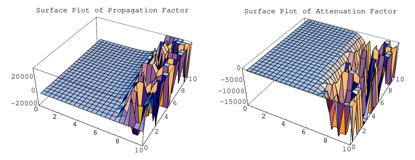
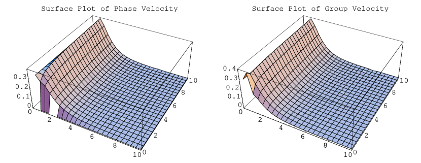
Figure 3: Dispersion is normal for waves with negligible angular frequencies.

In Figure 3, the wave number is infinite at the event horizon. The propagation factor decreases from the event horizon to $z=0.4$ and then increases to $z=6.25$. It takes random values in the region $6.25<z\leq 10$. The attenuation factor admits negative values in the region. The waves damp as they move away from the event horizon towards $z=0.55$ and grow afterwards up to $z=4.5$. The attenuation factor assumes random values in the region $4.5<z\leq 10$. The phase velocity of waves is less than the group velocity for the region $0<z\leq 5,~{}0.1\leq\omega\leq 5$ which implies anomalous dispersion. In the region $0\leq\omega<0.1$, the phase is moving faster than the group of wavelets and the dispersion is normal.

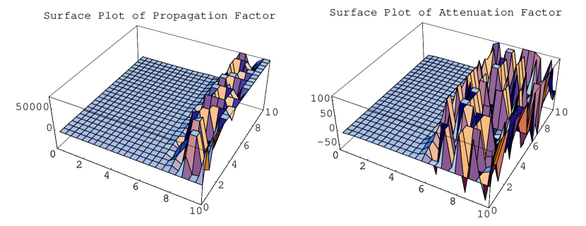
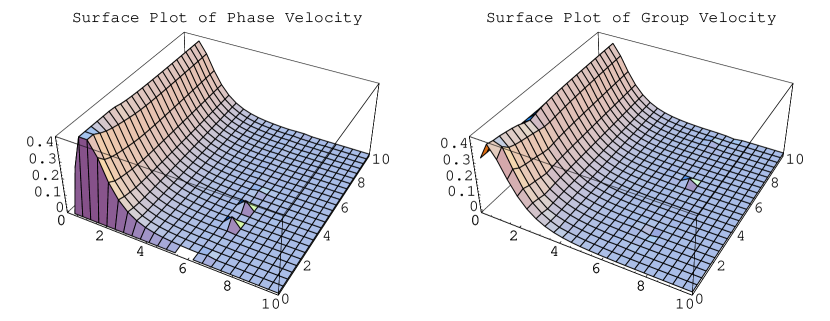
Figure 4: Many small regions admit normal and anomalous dispersion.

Figure 4 shows that no wave lies on the event horizon due to infinite wave number. The waves propagate rapidly with the increase in $z$ and $\omega$ in the region $6<z\leq 10$. The attenuation factor increases with the increase in $z$ and $\omega$ in the region $0<z\leq 4.25$ which shows that the waves damp with the increase in $z$ and $\omega$. The waves with negligible angular frequency do not show this behavior. The phase velocity exceeds the group velocity for the regions $0.55\leq z\leq 3,~{}5\leq\omega\leq 10$ and $1\leq z\leq 3,~{}0.15\leq\omega\leq 5$ which indicates normal dispersion. The group velocity is greater than the phase velocity for the region $0<z<0.55,~{}5\leq\omega\leq 10$ where dispersion is anomalous. In the regions $0\leq z<1,~{}0.15\leq\omega\leq 5$ and $0<z<0.15$, there lie random points of normal as well as anomalous dispersion.

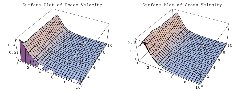
Figure 5: The region admits normal dispersion for most of the points. The waves with negligible angular frequencies show anomalous dispersion.

In Figure 5, the wave number is infinite at the event horizon. The propagation factor increases with the increase in $\omega$. It decreases in $0<z<1$ and increases in $1\leq z\leq 6.3$ with the increase in $z$ and takes random values in the region $6.3<z\leq 10$. In the region $0<z\leq 4.6$, the attenuation factor increases with the increase in $\omega$ and $z$. Thus the waves damp with the increase in the values of angular frequency and $z$. For $0<z\leq 4.8,~{}5\leq\omega\leq 10$ and $1\leq z\leq 4.8,~{}1\leq\omega\leq 2$, the phase velocity is greater than the group velocity and the dispersion is normal. Rest of the region possesses some points of anomalous dispersion but mostly admitting normal dispersion. The waves with angular frequency between $0$ and $0.1$ admit anomalous dispersion. The region $4.8<z\leq 10$ admits normal as well as anomalous points of dispersion.

5 Rotating Magnetized Background

For harmonic dependence of waves given by Eq.(2.1), the Fourier analysed GRMHD Eqs.(5.15)-(5.20) of [20] can be written as

$$c_{3}(\alpha^{\prime}+\iota k\alpha)-c_{2}\{(\alpha\lambda)^{\prime}+\iota k\alpha\lambda\}+c_{5}(\alpha V)^{\prime}$$

$$-c_{4}\{(\alpha u)^{\prime}-\iota\omega+\iota k\alpha u\}=0,$$ (5.1)

$$c_{5}\left(-\frac{\iota\omega}{\alpha}+\iota ku\right)=0,$$ (5.2)

$$c_{5}\iota k=0,$$ (5.3)

$$c_{1}\left(-\frac{\iota\omega}{\alpha}+\iota ku\right)+c_{2}\left\{-\frac{\iota\omega}{\alpha}\gamma^{2}u+\iota k(1+\gamma^{2}u^{2})+2\gamma^{4}u^{2}VV^{\prime}\right.$$

$$\left.-(1-2\gamma^{2}u^{2})(1+\gamma^{2}u^{2})\frac{u^{\prime}}{u}\right\}+c_{3}\gamma^{2}\left[\left(-\frac{\iota\omega}{\alpha}+\iota ku\right)V\right.$$

$$\left.+u\{(1+2\gamma^{2}V^{2})V^{\prime}+2\gamma^{2}uVu^{\prime}\}\right]=0,$$ (5.4)

$$c_{1}\rho\gamma^{2}u\{(1+\gamma^{2}V^{2})V^{\prime}+\gamma^{2}uVu^{\prime}\}-\frac{B^{2}}{4\pi}c_{4}\{(1-u^{2})\iota k+\frac{\alpha^{\prime}}{\alpha}(1-u^{2})-uu^{\prime}\}$$

$$+c_{2}\left[-\left(\rho\gamma^{4}uV-\frac{\lambda B^{2}}{4\pi}\right)\frac{\iota\omega}{\alpha}+\iota ku\left(\rho\gamma^{4}uV+\frac{\lambda B^{2}}{4\pi}\right)+\frac{B^{2}u}{4\pi\alpha}(\lambda\alpha)^{\prime}\right.$$

$$\left.+\rho\gamma^{2}\{(1+2\gamma^{2}u^{2})(1+2\gamma^{2}V^{2})-\gamma^{2}V^{2}\}V^{\prime}+2\rho\gamma^{4}(1+2\gamma^{2}u^{2})uVu^{\prime}\right]$$

$$+c_{3}\left[-\left\{\rho\gamma^{2}(1+\gamma^{2}V^{2})+\frac{B^{2}}{4\pi}\right\}\frac{\iota\omega}{\alpha}+\iota ku\left\{\rho\gamma^{2}(1+\gamma^{2}V^{2})-\frac{B^{2}}{4\pi}\right\}\right.$$

$$\left.+\rho\gamma^{4}u\{(1+4\gamma^{2}V^{2})uu^{\prime}+4(1+\gamma^{2}V^{2})VV^{\prime}\}-\frac{B^{2}u\alpha^{\prime}}{4\pi\alpha}\right]=0,$$ (5.5)

$$c_{1}\rho\gamma^{2}[a_{z}+u\{(1+\gamma^{2}u^{2})u^{\prime}+\gamma^{2}VuV^{\prime}\}]$$

$$+c_{2}\left[-\left\{\rho\gamma^{2}(1+\gamma^{2}u^{2})+\frac{\lambda^{2}B^{2}}{4\pi}\right\}\frac{\iota\omega}{\alpha}+\left\{\rho\gamma^{2}(1+\gamma^{2}u^{2})-\frac{\lambda^{2}B^{2}}{4\pi}\right\}\iota ku\right.$$

$$\left.+\left\{\rho\gamma^{2}\{u^{\prime}(1+\gamma^{2}u^{2})(1+4\gamma^{2}u^{2})+2u\gamma^{2}((1+2\gamma^{2}u^{2})VV^{\prime}+a_{z})\}\right.\right.$$

$$\left.\left.-\frac{\lambda B^{2}u}{4\pi\alpha}(\alpha\lambda)^{\prime}\right\}\right]+c_{3}\left[-\left(\rho\gamma^{4}uV-\frac{\lambda B^{2}}{4\pi}\right)\frac{\iota\omega}{\alpha}+\left(\rho\gamma^{4}uV+\frac{\lambda B^{2}}{4\pi}\right)\iota ku\right.$$

$$\left.+\left\{\rho\gamma^{4}\{u^{2}V^{\prime}(1+4\gamma^{2}V^{2})+2V(a_{z}+uu^{\prime}(1+2\gamma^{2}u^{2}))\}+\frac{\lambda B^{2}\alpha^{\prime}u}{4\pi\alpha}\right\}\right]$$

$$+\frac{B^{2}}{4\pi}c_{4}\left[\lambda(1-u^{2})\iota k+\lambda\frac{\alpha^{\prime}}{\alpha}(1-u^{2})-\lambda uu^{\prime}+\frac{(\lambda\alpha)^{\prime}}{\alpha}\right]=0.$$ (5.6)

Equations (5.2) and (5.3) imply that $c_{5}$ is zero which gives that $b_{z}$ is zero.

5.1 Numerical Solutions

We have assumed the same velocity which we have taken in the previous section. In addition to this, we consider the same magnetic field components which we have used in the case of isothermal fluid in [22], i.e., $B_{x}=B\lambda=-\sqrt{\frac{88(1-\tanh^{4}(z))}{7\tanh^{2}(z)}}$ and $B_{z}=B=\sqrt{\frac{88}{7}}$.

Under these conditions, when we solve the determinant of Eqs.(LABEL:l1), (5)-(5) by using $c_{5}=0$, we obtain a dispersion relation which leads to four complex wave numbers $k$. These wave numbers are shown in Figures 6-9.

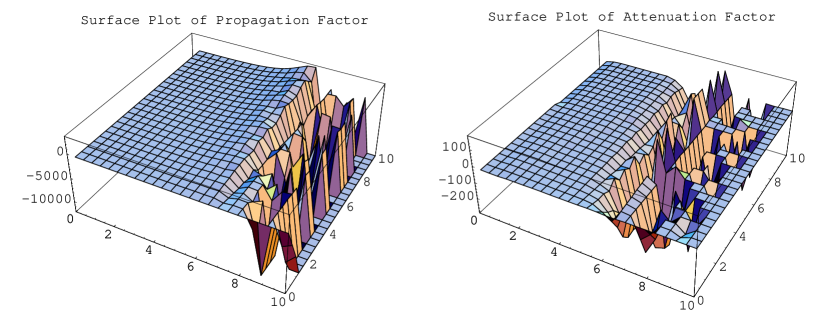
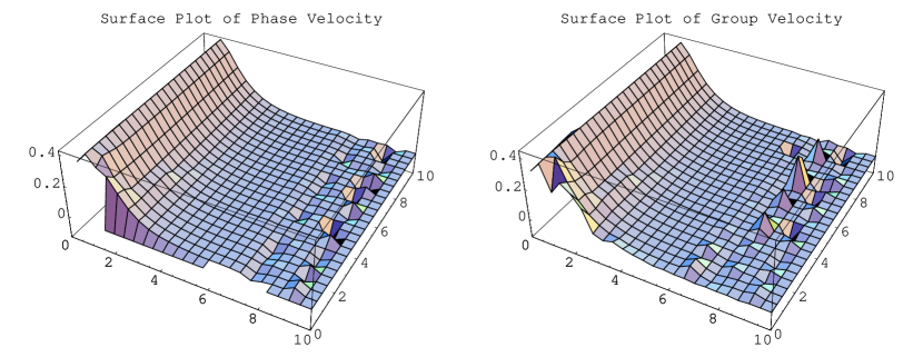
Figure 6: Wave propagation is less near the event horizon. Anomalous dispersion occur in most of the region.

Figure 6 indicates that the wave number is infinite at the event horizon. The propagation factor has small values near the event horizon. It suddenly increases and then decreases as the waves move towards $z=1$ after which it increases in the region $0<z<6.3$. This shows that the waves abruptly move faster, then their propagation decreases and afterwards increases as they move away from the event horizon in the mentioned region. The propagation of the waves is fast as we increase their angular frequency which is quite usual. The propagation factor takes random values in the region $6.3\leq z\leq 10$. The attenuation factor increases when the waves move away from the event horizon. It decreases in $0.3\leq z\leq 0.7$ and then increases monotonically in the region $0<z\leq 4,~{}1\leq\omega\leq 10$. Thus damping occurs when the waves move away from the event horizon. The waves grow in the region $0.3\leq z\leq 0.7$ after which they show smooth damping.

The phase velocity is less than the group velocity for the waves near the event horizon which shows normal dispersion. As the waves move away from the event horizon, the group velocity overcomes the phase velocity and anomalous dispersion holds. The waves with low angular frequency admit anomalous dispersion. As the angular frequency increases, the waves show normal dispersion near the event horizon but as these waves move away, they disperse anomalously. Thus these waves cannot transfer any information out of the region.

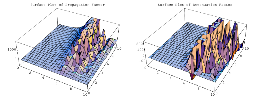
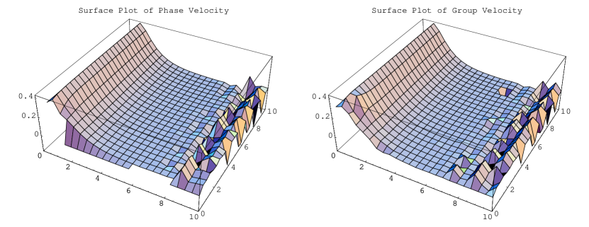
Figure 7: Dispersion is random in most of the region. Negative wave propagation region is observable.

Figure 7 demonstrates that the wave number is infinite at $z=0$ and thus no wave exists there. The propagation factor decreases abruptly when the waves move away from the event horizon. This factor increases with an increase in the value of $z$ and $\omega$. This means that the wave propagation abruptly decreases when the waves move away from the neighborhood of the event horizon of the Schwarzschild black hole. Then their propagation increases gradually. The waves with higher angular frequency propagate more rapidly in the environment than the waves with lower angular frequency. The attenuation factor decreases when moving away from the event horizon till $z=0.5$. It then increases a little and decreases gradually in the region $0<z\leq 2,~{}2\leq\omega\leq 10$. The waves grow as they move away from the event horizon, a little damping occurs after which they grow again in this region. In the rest of the region, the growth and damping occur randomly.

The group velocity is greater than the phase velocity in the region $2\leq z\leq 10,~{}4\leq\omega\leq 10$ which indicates anomalous dispersion. The rest of the region shows random points of dispersion. In the region $8\leq z\leq 10$, the phase as well as the group velocity admit the negative values.

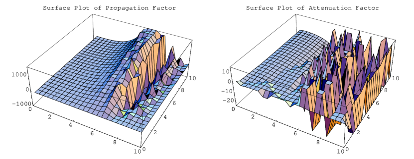
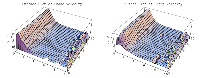
Figure 8: Small regions of normal as well as anomalous dispersion are found. Negative wave propagation region occur.

Figure 8 indicates that when the waves move away from the event horizon, the propagation factor decreases towards $z=1$ and increases gradually towards $z=6$. In the region $6<z\leq 10$, the propagation factor attains random values and in the region $0<z\leq 2,~{}2\leq\omega\leq 10$, the attenuation factor decreases as $z$ increases. This indicates that the waves damp with the increase in $z$ in this small region. In the rest of the region, the attenuation factor admits random values and thus the growth and damping of waves occur at random.

The phase velocity is greater than the group velocity for most of the points in the regions $2\leq z\leq 3,~{}0.5\leq\omega\leq 4$ and $3\leq z\leq 4,~{}1\leq\omega\leq 6$ which indicates normal dispersion. The group velocity exceeds the phase velocity and the dispersion is normal in the regions (i) $1\leq z\leq 2,~{}2\leq\omega\leq 10$, (ii) $2\leq z\leq 3,~{}4\leq\omega\leq 10$ and (iii) $3\leq z\leq 3.5,~{}6\leq\omega\leq 10$. The rest of the region contains points of normal as well as anomalous dispersion. The region $6\leq z\leq 10$ takes some points at which the phase as well as the group velocity have negative values.

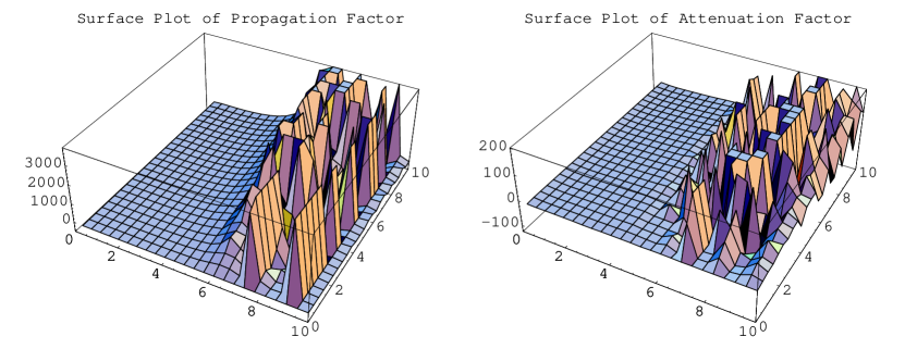
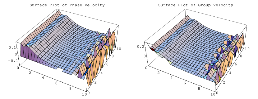
Figure 9: Most of the regions contains random points of dispersion. Region with negative phase velocity propagation is also present.

In Figure 9, the wave number is infinite at $z=0$. The propagation factor decreases at once on going away from the event horizon. It increases gradually when the value of $z$ as well as the angular frequency increase in the region. This means that the propagation of waves decreases abruptly when they move away from the event horizon. and increases when the waves move faster. The waves with higher angular frequency propagate faster than the waves with lower angular frequency. The propagation factor assumes random values in the region $6\leq z\leq 10$. The attenuation factor has less variations in the region $0<z\leq 4$ and shows increasing behavior as the value of $z$ and $\omega$ increases. This means that the waves damp either when they move away from the event horizon or when their angular frequency is increased. The variation of this factor is much more in the region $4<z\leq 10$.

In the regions (i) $0<z<3,~{}4\leq\omega\leq 10$, (ii) $1\leq z<4,~{}2\leq\omega\leq 4$ and (iii) $0<z\leq 2.5,~{}2\leq\omega\leq 4$, the phase velocity is greater than the group velocity and the dispersion is normal. The regions $3\leq z\leq 4.4,~{}4\leq\omega\leq 10$ and $2.5\leq z\leq 5,~{}2\leq\omega\leq 4$ possess anomalous dispersion due to the fact that the group velocity is greater than the phase velocity. The regions $0\leq\omega\leq 2$ and $4.4<z\leq 10$ admit some points with normal and some with anomalous dispersion. In the region $5<z\leq 10$, the phase velocity takes negative values at some points and hence the region contains points with negative phase velocity propagation.

6 Outlook

In this paper, we work out the complex wave numbers near the event horizon of the Schwarzschild black hole. For this purpose, we have taken the planar analogue of the Schwarzschild spacetime with non-rotating and rotating, non-magnetized and magnetized backgrounds. We have investigated [20] real dispersion relations for the same backgrounds by using Rindler coordinates. The Rindler coordinates give best approximation of the Schwarzschild spacetime near the event horizon whereas this planar analogue is valid for the whole accretion cloud around the Schwarzschild event horizon. The properties of the surrounding plasma are based on the complex wave numbers.

The summary of the results obtained is outlined below:

• The wave number is infinite at the horizon which supports the well-known fact that no information can be extracted from a black hole.

• There is no difference in the dispersion relations whether the plasma is magnetized or not, in the case of non-rotating background because the gravity produces no perturbations in the magnetic field. The fluid is dispersed normally in only one case (Figure 2) which allows the waves to pass through this region. The waves show anomalous dispersion in the other case.

• The rotating background exhibits negative phase velocity propagation regions far away from the black hole event horizon. It seems that the black hole’s gravity ceases the waves to admit the negative phase velocity propagation region. For the region with larger values of $z$, the dispersion is found to be normal at some points and anomalous at some other points. This creates a doubt whether all the waves can get out of this region.

• There is only one case (Figure 5) in which normal dispersion occurs at most of the points in rotating non-magnetized background.

• For the rotating magnetized background, many small regions which admit normal dispersion are found. These regions are surrounded by the regions of anomalous dispersion and hence no information can be extracted from these regions.

The comparison of the results with those obtained from the previous literature is given as follows:

• When we compare our results to that of [20], we find that in non-rotating background we have detected the anomaly of waves which was not recognized previously. In the case of rotating magnetized background we obtain the negative phase velocity propagation region far away from the event horizon whereas in [20], the whole region admits this property.

• In the case of non-rotating isothermal plasma [21], the dispersion is anomalous in all the cases whereas in cold plasma the region with normal dispersion is also found. It can be deduced that the plasma pressure ceases the chances of waves to come out of the region in the neighborhood of the event horizon in pure Schwarzschild background.

• In the case of rotating magnetized isothermal plasma [22], the medium admits normal dispersion of waves in plasma surrounding the event horizon for the waves admitting high angular frequency. For the same case of cold plasma, the regions with normal dispersion are enclosed by the regions admitting anomalous dispersion of the waves. For the restricted Kerr black hole, it can be observed that the pressure reduction ceases the chances of waves to pass through the region.

We conclude that no information can be extracted from the Schwarzschild event horizon. There are chances to collect the information from the exterior of the event horizon of the Schwarzschild black hole for the case of cold plasma. In the case of the restricted Kerr geometry, the cold plasma does not allow the waves to pass through in most of the cases. However, there are little chances for the waves to move out of the accretion disk.

Acknowledgment

We appreciate the Higher Education Commission Islamabad, Pakistan, for its financial support during this work through the Indigenous PhD 5000 Fellowship Program Batch-II.

References

- [1] Petterson, J.A.: Phys. Rev. D10(1974)3166.
- [2] Arnowitt, R., Deser, S. and Misner, C.W.: Gravitation: An Introduction to Current Research ed. Witten, L. (Wiley, New York, 1962).
- [3] Stachel, J.: Acta. Phys. Polon. 35(1969)689.
- [4] Smarr, L. and York, J.W., Jr.: Phys. Rev. D17(1978)2529.
- [5] York, J.W., Jr.: Sources of Gravitational Radiation ed. Smarr, L. (Cambridge University Press, Cambridge, 1979).
- [6] Smarr, L., Taubes, C. and Wilson, J.R.: Eassays in General Relativity, A Festschrift for Ibraham Taub, ed. Tipler, F. (Academic Press, New York, 1980).
- [7] Evans, C.R., Smarr, L.L. and Wilson, J.R.: Astrophysical Radiation Hydrodynamics ed. Norman, M. and Winkler, K.H. (Reidel, Dordrecht, 1986).
- [8] Thorne, K.S. and Macdonald, D.A.: Mon. Not. R. Astron. Soc. 198(1982)339.
- [9] Thorne, K.S. and Macdonald, D.A.: Mon. Not. R. Astron. Soc. 198(1982)345.
- [10] Black Holes: The Membrane Paradigm eds. Thorne, K.S., Price, R.H. and Macdonald, D.A. (Yale University Press, New Haven, 1986).
- [11] Holcomb, K.A. and Tajima, T.: Phys. Rev. D40(1989)3809.
- [12] Holcomb, K.A.: Astrophys. J. 362(1990)381.
- [13] Dettmann, C.P., Frankel, N.E. and Kowalenko, V.: Phys. Rev. D48(1993)5655.
- [14] Sakai, J. and Kawata, T.: J. Phys. Soc. Jpn. 49(1980)747.
- [15] Khanna, R.: Mon. Not. R. Astron. Soc. 294(1998)673.
- [16] Zhang, X.-H.: Phys. Rev. D39(1989)2933.
- [17] Zhang, X.-H.: Phys. Rev. D40(1989)3858.
- [18] Buzzi, V., Hines, K.C. and Treumann, R.A.: Phys. Rev. D51(1995)6663.
- [19] Buzzi, V., Hines, K.C. and Treumann, R.A.: Phys. Rev. D51(1995)6677.
- [20] Sharif, M. and Sheikh, U: Gen. Relat. Gravit. 39(2007)1437.
- [21] Sharif, M. and Sheikh, U: Effects of Schwarzschild Geometry on Isothermal Plasma Wave Dispersion, submitted for publication.
- [22] Sharif, M. and Sheikh, U: Effects of Rotating Background on Isothermal Plasma Wave Dispersion in Schwarzschild Geometry, submitted for publication.
- [23] Achenbach, J.D.: Wave Propogation in Elastic Solids (North-Holland Publishing Company, Oxford, 1973).