About combinatorics, and observables

Andrea Gregori^†
Abstract
We investigate the most general “phase space” of configurations, consisting of all possible ways of assigning elementary attributes, “energies”, to elementary positions, “cells”. We discuss how this space possesses structures that can be approximated by a quantum physics scenario. In particular, we discuss how the Heisenberg’s “Uncertainty Principle” and a “universe” with a three-dimensional space arise, and what kind of mechanics rules it.

 ^†e-mail: agregori@libero.it

1 Introduction

In a recent work [1] we have discussed how, considering the superposition of all possible string configurations, weighted with their occupation in the string phase space, we recover the actual properties and physics of the Universe, as they are observed at present time and along its history and evolution. At any time, the main contribution to the mean values of observables comes from the string configurations of minimal entropy. We have seen how this leads to a viable phenomenological scenario, highly predictive and compatible with current experiments. In this work, we approach the problem from a different, more general perspective: we investigate the most general possible phase space of “spaces”, of arbitrary volume and number of coordinates, describing whatever kind of degrees of freedom, asking ourselves if in this apparently indistinct “night of everything” it is possible to disentangle particular structures that appear more frequently than other ones.

We are used to order our observations according to phenomena that take place in what we call space-time. An experiment, or, better, an observation (through an experiment), basically consists in realizing that something has changed: our “eyes” have been affected by something, that we call “light”, that has changed their configuration (molecular, atomic configuration). This light may carry information about changes in our environment, that we refer either to gravitational phenomena, or electromagnetic ones, and so on… In order to explain them we introduce energies, momenta, “forces”, i.e. interactions, and therefore we speak in terms of masses, couplings etc… However, all in all, what all these concepts refer to is a change in the “geometry” of our environment, a change that “propagates” to us, and eventually results in a change in our brain, the “observer”. String Theory marks a big step forward along this line of thoughts, in that it introduces a geometric origin of particles, masses, fields and couplings, which basically turn out to be geometric degrees of freedom, of an “internal” space. In short, it implements the degrees of freedom of the geometries of the space, and their changes during time (in one word, the “space-time”) in a fibered space. In its basic formulation, base and fiber appear on the same footing. It remains however that the “conjugates” variables to space and time, namely energy and momentum, are introduced “by hand”, as separate concepts, related to the modes of expansion of the string. Indeed, in order to introduce them, besides the “target space” we precisely need the “string”, the object that “lives” in this spaces. Since the time it was realized that the various perturbative string constructions belong to a net of slices of a unique theory, which in certain limits (11d supergravity) is not based on the introduction of a string, and in other dual approaches it requires more extended objects in order to express all its degrees of freedom (membranes), it seems the more and more reasonable to think that these objects are in themselves not so fundamental, being perhaps just convenient “parametrizations” of the real thing. This appears to be the parametrization of a geometric problem. On the other hand, since the time of General Relativity we know that energy and geometry are related, and “interchangeable”. Understanding energy is therefore the same as understanding geometry.

But what is after all geometry other than a way of saying that, by moving along a path in space, we will encounter or not some modifications? Assigning a “geometry” is a way of parametrizing modifications, differentiations, “unevenesses”, through a map from a space of “attributes”, whose coordinate we call “curvature”, to another space, that we call “the” space. When we speak of “attributes”, we mean the very basic possibility of assigning an “elementary object” belonging to a set, a “space”, to “positions”, “elementary cells” of a target set/space. An elementary cell can either be occupied or not, by being assigned an elementary object or not. We deal therefore with a “combinatoric of the distribution of occupations of cells”. Indeed, had we to start with a generic “phase space of everything”, in order to recognize structures inside this space we should be able to measure, to say without ambiguity if something is larger, equal or smaller than something else. In practice, we should get rid of infinities, introduce a regulator (this is by the way what one does any time, when it is a matter of performing physical computations in spaces with infinitely many degrees of freedom) . This would be done by working with a finite, although arbitrary, number $n$ of coordinates, in a finite, although arbitrary volume $V$. In order to measure things, we should also introduce a “length” $\ell$, the size of the “elementary cell”, such that volumes of submanifolds or subsets of this space would be “counted” in terms of $v_{(p)}=(\ell)^{p}$, $1\leq p\leq n$. In order to “count” degrees of freedom, we must work with discrete quantities, reduce the space to a lattice. In itself an elementary cell is “adimensional”, in the sense that, expressing volumes of any space dimensionality in terms of number of cells, we can compare any powers of length. Only in this way we can really say if a “segment” may contain more or less degrees of freedom than another one, and we can also compare without ambiguity the size of a “segment” to the one of a discrete set of “points”. In this way, we can deal with any kind of geometry.

In this work, we assume that the basic formulation of the problem is the discrete one, given in terms of “unit cells”, and investigate the combinatorics of the applications of “cells into cells”. We consider therefore a space in which everything is given in terms of number of “cells”: a point is one cell, a two-dimensional square is given by $N\times N$ cells etc… There are no units a priori distinguishing the measure of space from the one of its attributes (in other words, “space” and “momentum/energy” are measured in the same way, in terms of unit cells). The problem of geometries becomes in this way a problem of combinatorics, and of their interpretation. We start our analysis in section 2 by investigating the combinatorics of the “distribution of attributes”, namely, the applications of “cells” into a space of “positions of cells”, and discuss how, and in which sense, certain structures dominate. This allows to see an “order” in this “darkness”. We discuss how a “geometry” shows up, and how geometric inhomogeneities, that we can interpret as the discrete version of “wave packets”, arise. We recover in this way, through a completely different approach, all the known concepts of particles and masses. In the “phase space” constituted by all possible configurations we introduce a “time ordering” based on the inclusion of sets of configurations. At any time, what appears to be the “Universe” is the superpositions of an infinite number of configurations, weighted according the their “geometric” occupation in the phase space, namely by the exponential of their entropy. Evaluation of entropies enables to see that three space dimensions are favoured; statistically, the “space-time” looks therefore mostly “four dimensional”.

Time evolution turns out to be neither deterministic, nor probabilistic. On the other hand, under certain conditions, after the introduction of approximations and simplifications enabling one to concretely solve the combinatoric problem with a viable effective theory, one is led to the probabilistic interpretation usually associated to quantum mechanics. Indeed, the Heisenberg’s Uncertainty Principle shows up as an inequality encoding the indeterminacy introduced by ignoring the contribution to the mean values due to a full bunch of configurations, for which there is no interpretation in terms of particles and fields, interacting in a space-time of well defined dimensionality. The Uncertainty Principle turns out to be not only a bound on our possibility of measuring quantities, but a bound on the meaning in itself of these quantities. It arises not simply as a bound on the precision with which we can know certain observables, but as the threshold beyond which they cannot even be consistently defined. In a certain sense, they make sense only as “mean, average values” we can introduce only together with a certain degree of “fuzziness”.

We devote section 4 to a discussion of the issues of causality and in what limit “quantum mechanics” arises in this framework. We pass then (section 5) to discuss what is the role played by string theory in this scenario: in which sense and up to what extent it provides an approximation to the description of the combinatoric/geometric scenario, of which Quantum String Theory constitutes an implementation in the framework of a continuum (differentiable) space. Strictly speaking, String Theory deals only with a subset of configurations, a subspace of the full phase space, but, through the implementation of quantization, and therefore of the Heisenberg’s Uncertainty Principle, it considers also the neglected configurations of the phase space, relating them to the uncertainty “built in” in its basic definition. In other words, it comes already provided with a “fuzziness” that incorporates in its range the contribution of all the other possible configurations.

We briefly reconsider the basics of string theory in this perspective, discussing the relation to the “combinatoric” approach. In particular, we reconsider (section 6) the entropy weighted sum of Ref. [1]; we point out how, at “fixed time”, the entropy of a string vacuum, intended as the entropy of the states a string configuration is built of, computed according to their probability within the string vacuum, is “dual” to the entropy of the whole string configuration itself, viewed as an element in the space of all the possible configurations. As a consequence, the most often realized string configurations, those of maximal “absolute” entropy, correspond to those of minimal “string” entropy, as expressed in the functional of Ref. [1]. Indeed, string theory gives a “collective” representation of configurations in phase space, centered on effective “mean values” of geometries and inhomogeneities (parametrized through particles, fields, and their masses and charges), embedded in a space already provided with a “time” coordinate. However, in the perturbative string constructions the latter appears to be in a “decompactification phase”, and does not coincide with the “physical time” parametrizing the evolution in the full phase space. The identification works only for the string configurations of minimal entropy, which represent somehow the “on shell” description of the Universe. Along the path of minimal string entropy (or maximal phase space entropy) configurations, the “average” geometry of the universe is that of a three-dimensional sphere. Near-to-minimal configurations contribute on the other hand for inhomogeneities that give rise to “local concentrations” of energy/curvature: particles, wave packets, galaxy clusters etc… These perturbations of the “regular” geometry are of the order of the Heisenberg’s Uncertainties.

In section 7 we discuss how the Universe, as it appears to an observer, builds up; in particular, we discuss what is the meaning of a boundary, an horizon, in such a spheric geometry, and the non-trivial relation between what one sees, and what indeed is inside this space.

This work is thought as complementary of [1]. Therefore, many discussions are not repeated here, and the reader is invited to refer to [1] in order to complete the information.

2 The general set up

Consider the system constituted by the following two ”cells”:

(2.1)

Let’s assume that the only degrees of freedom this system possesses are that each one of the two cells can independently be white or black. We have the following possible configurations:

(2.2)

(2.3)

(2.4)

(2.5)

This is the “phase space” of our system. The configuration “one cell white, one cell black” is realized two times, while the configuration “two cells white” and “two cells black” are realized each one just once. Let’s now abstract from the practical fact that these pictures appear inserted in a page, in which the presence of a written text clearly selects an orientation. When considered as a “universe”, something standing alone in its own, configuration 2.3 and 2.4 are equivalent. In the average, for an observer possessing the same “symmetry” of this system (we will come back later to the subtleties of the presence of an observer), the “universe” will appear something like the following:

(2.6)

or, equivalently, the following:

(2.7)

namely, the “sum”:

(2.8)

or equivalently the sum:

(2.9)

Notice that the observer “doesn’t know” that we have rotated the second and third term, because he possesses the same symmetries of the system, and therefore is not able to distinguish the two cases by comparing the orientation with, say, the orientation of the characters of the text. What he sees, is a universe consisting of two cells which appear slightly differentiated, one “light grey”, the other “dark grey”.

The system just described can be viewed as a two-dimensional space, in which one coordinate specifies the position of a cell along the “space”, and the other coordinate the attribute of each position, namely, the colour. Our two-dimensional “phase space” is made by $2({\rm space})\times 2({\rm colours})$ cells. By definition the volume occupied in the phase space by each configuration (two white; two black; one white one black) is proportional to the logarithm of its entropy. The highest occupation corresponds to the configuration with highest entropy. The effective appearance, one light-grey one dark-grey, 2.6 or 2.7, mostly resembles the highest entropy configuration.

Let’s now consider in general cells and colours. The colours are attributes we can assign to the cells, which represent the positions in our space. On the other hand, these “degrees of freedom” can themselves be viewed as coordinates. Indeed, if in our space with $m({\rm space})\times n({\rm colours})$ we have $n>m$, then we have more degrees of freedom than places to allocate them. In this case, it is more appropriate to invert the interpretation, and speak of $n$ places to which to assign the $m$ cells. The colours become the space and the cells their “attributes”. Therefore, in the following we consider always $n\leq m$.

2.1 Distributing degrees of freedom

Consider now a generic “multi-dimensional” space, consisting of $M_{1}^{p_{1}}\times\ldots\times M_{i}^{p_{i}}\ldots\times M_{n}^{p_{n}}$ “elementary cells”. Since an elementary, “unit” cell is basically a-dimensional, it makes sense to measure the volume of this $p$-dimensional space, $p=\sum^{n}_{i}p_{i}$, in terms of unit cells: $V=M_{1}^{p_{i}}\times\ldots\times M_{n}^{p_{n}}\stackrel{{\scriptstyle\rm def}}{{\equiv}}M^{p}$. Although with the same volume, from the point of view of the combinatorics of cells and attributes this space is deeply different from a one-dimensional space with $M^{p}$ cells. However, independently on the dimensionality, to such a space we can in any case assign, in the sense of “distribute”, $N\leq M^{p}$ “elementary” attributes. Indeed, in order to preserve the basic interpretation of the “$N$” coordinate as “attributes” and the “$M$” degrees of freedom as “space” coordinates, to which attributes are assigned, it is necessary that $N\leq M_{n}$, $\forall\,n$ . What are these attributes? Cells, simply cells: our space doesn’t know about “colours”, it is simply a mathematical structure of cells, and cells that we attribute in certain positions to cells. By doing so, we are constructing a discrete “function” $y=f(\vec{x})$, where $y$ runs in the “attributes” and $\vec{x}\in\{M^{\otimes p}\}$ belongs to our $p$-dimensional space. We define the phase space as the space of the assignments, the “maps”:

$$N\,\to\,\prod_{i}\otimes M_{i}^{\otimes p_{i}}\,,~{}~{}~{}~{}~{}M_{i}\,\geq\,N\,.$$ (2.10)

For large $M_{i}$ and $N$, we can approximate the discrete degrees of freedom with continuous coordinates: $M_{i}\to r_{i}$, $N\to R$. We have therefore a $p$-dimensional space with volume $\prod r_{i}^{p_{i}}$, and a continuous map $\vec{x}\in\{\vec{r}^{\vec{p}}\}\stackrel{{\scriptstyle f}}{{\to}}y\in\{R\}$, where $y$ spans the space up to $R=\prod r_{i}^{p_{i}}\equiv r^{p}$ and no more. In the following we will always consider $M_{i}\gg N$, while keeping $V=M^{p}$ finite. This has to considered as a regularization condition, to be evetually relaxed by letting $V\to\infty$. We ask now: what is the most realized configuration, namely, are there special combinatorics in such a phase space that single out “preferred” structures, in the same sense as in our “two-cells $\times$ two colours” example we found that the system in the average appears “light-grey–dark-grey”? In order to come out of this complicated combinatoric problem, let’s call $y$ “total energy”. The value $y$ is given by the total number of unit cells of this coordinate. Measured in units of the elementary cell, energy goes from $1$ to $N\sim R$. Distributing, assigning cells from our “energy coordinate” to our $p$-dimensional space corresponds then to assigning a curvature, a “geometry” to this space. Indeed, for us assigning a geometry will be equivalent to assigning an energy distribution. In this perspective, a curved surface in $p$ dimensions has not to be seen as a geometric set of points embedded in a $p+1$-dimensional flat space, but as a particular configuration due to a distribution of the energy cells along the coordinates of the $p$-dimensional space $\prod M_{i}^{p_{i}}$, $\sum p_{i}=p$, which we interpret in geometric terms as a curved space. This entails an implicit choice of units of energy as compared to units measuring space, that we now consider as simply set to 1, as is done in quantum-relativistic mechanics when choosing the so-called reduced Planck units: $c=\hbar=M_{pl}=1$. The geometry of a $p$-sphere of radius $r$ is therefore characterized by an energy density scaling like:

$$\rho(E)~{}\approx~{}K(p)\,{N\over r^{p}}\;\propto\;{1\over r^{2}}\,,$$ (2.11)

where $K(p)$ is a typical symmetry factor depending on the dimensionality of the sphere. At any given $N$ (and fixed volume $V\gg N$), the most entropic configurations are the “maximally symmetric” ones, i.e. those that look like spheres in the above sense. Equation 2.11 sets also a bound on the mean amount of energy we can put within a space region of radius $r$ at any dimension $p$. If we try to force more energy to stay within such a region, we “overcurve” it, producing a less symmetric configuration (see figure 1).

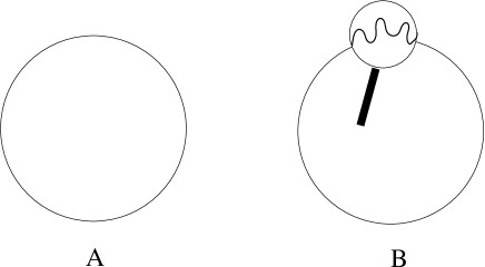
Figure 1: On the left (A) is drawn a sphere (here for simplicity a 1-sphere, a circle, on the right (B) a surface with more energy (curvature) than a sphere, here showing out under a “loupe” as a wavy line.

For $p=3$, equation 2.11 reads:

$$E_{p=3}\,(\sim N)~{}\propto~{}r\,.$$ (2.12)

In classical terms, this is basically the Schwarzschild bound relating the radius of a Black Hole to its mass (= total rest energy). In practice, we are saying that configurations over the Schwarzschild bound (as well as configurations below this bound) are less entropic, unfavoured in the phase space as compared to the spheres. We will come back on this issue later in this work.

2.2 Entropy of spheres

We want to see now what is the entropy, or equivalently, the weight $W$ in the phase space, of a $p$-sphere of radius $m$. As it was in the previous section for the total energy $N$, here too we consider $m\ll M$. The weight of a sphere in the phase space will be given by the number of times such a sphere can be formed by permuting its points, times the number of choices of the position of, say, its center, in the whole space. Since we eventually are going to take the limit $V\to\infty$, we don’t consider here this second contribution, which is going to produce an infinite factor, equal for each kind of geometry, for any finite amount of total energy $N$. We will therefore concentrate here to the first contribution, the one that distinguishes from sphere to sphere, and from sphere to other geometries. To this purpose, we solve the “differential equation” (more properly, a finite difference equation) of the increase in the combinatoric when passing from $m$ to $m+1$. In a $p$-dimensional space, illustrated as a “$p$-cube” in figure 2,

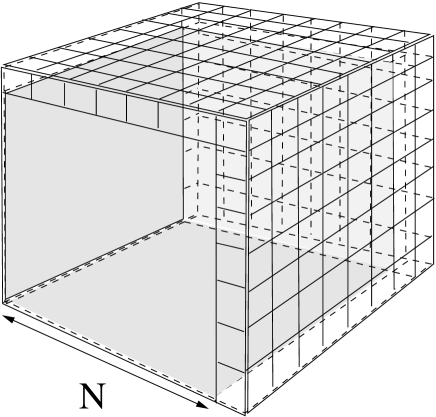
Figure 2: The growth from $m\to m+1$ of a “$p$ cube”, here schematically represented as a 3-cube.

when we pass from $m$ to $m+1$ we increase the volume by an amount of cells scaling as the boundary of the space. For instance, in the case of a three-cube we get some $3m^{2}$ more cells. We can think to place the one more degree of freedom in one of these cells, but we can also permute the position of the planes, while a subspace of volume $m^{p}$ has the same distribution of cells as before (see figure 3).

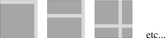
Figure 3: The new cells, represented in white in figure 2, and schematically represented here in light grey in a projection to two dimensions, can be added in any position of the cube.

We have therefore $\sim(m+1)^{p}$, and not only $\sim pm^{p-1}$ possibilities. In order to preserve the type of geometry, we must multiply the new gained volume times the “matter density” of the sphere, $\sim 1/m^{2}$. We recall in fact that in this framework boundary conditions, such as for instance those allowing to conclude that we have the curved geometry of a sphere, are not to be thought as geometric conditions to be imposed on the coordinates, as if a geometry could exist independently of the energy content of space. A sphere is by definition identified with the space with an energy density corresponding to (i.e. generating) the appropriate curvature. In this way one can see that:

$$W(m+1)\,\sim\,W(m)\times{(m+1)^{p}\over m^{2}}\,.$$ (2.13)

The rate of increase of the number of configurations scales therefore like:

$$W(m+1)_{p-{\rm sphere}}\,\approx\,W(m)_{p-{\rm sphere}}\times m^{p-2}\,,~{}~{}~{}~{}p\,\geq\,2\,,$$ (2.14)

where on the second factor of the r.h.s. we have been a bit loose in the evaluation of the exact volumes, neglecting minorities like a difference between $m$ and $m+1$ and the correct normalization of the curvature/energy density of a $p$-sphere: what we are interested in is understanding the main behaviour at large $m$. Translated into a difference equation, 2.14 means:

$${\Delta W(m)_{p}\over W(m)_{p}}\,\sim\,\,m^{p-2}\,,~{}~{}~{}~{}p\,\geq\,2\,.$$ (2.15)

Through a passage to differential equations, $m\to x$, $x$ a continuous variable, we can integrate and obtain:

$$S_{(p\geq 2)}\,\propto\,\ln W(m)\,\sim\,{1\over p-1}\,m^{p-1}\,.$$ (2.16)

We obtain therefore the typical scaling law of the entropy of a $p$-dimensional black hole (see for instance [2]).

For $p=1$, we cannot have a sphere. With an energy density $\rho(E)$ scaling as $1/R^{2}$, the total energy in one dimension would be $E\sim\rho(E)\times R\sim 1/R$, but we cannot have a total energy $E\sim 1/R$, lower than one. The only possible configurations are “less symmetric” than a sphere. For a total energy $N=m=R$ there is no free space at all: $m$ cells can only occupy the $m$ free positions, and therefore $\Delta W=0$. In general, for any energy $n<m$ that anyway scales proportionally to $m$: $n/m=q$, we have:

$$W(m+1)_{1}\,\sim W(m)_{1}\times q\,,$$ (2.17)

and therefore:

$$dW/W~{}\sim~{}0\,,~{}~{}~{}~{}~{}~{}p=1\,,$$ (2.18)

leading to:

$$S_{(p=1)}\,\propto\,\ln W~{}\sim~{}{\rm const.}$$ (2.19)

This analysis allows us to conclude that:

• At any energy $N$, the most entropic configuration is the one corresponding to the geo-

  metry of a three-sphere.

Higher dimensional spheres have an unfavoured ratio entropy/energy. Three dimensions are then statistically “selected out” as the dominant space dimensionality. In higher dimension $p$, the condition for having a sphere of radius $r\sim m$ reads in fact:

$${N\over m^{p}}\,\sim\,{1\over m^{2}}\,,$$ (2.20)

which implies that the radius must be shorter than the total energy:

$$m\,\sim\,N^{1\over p-2}~{}<\,N\,,~{}~{}~{}p>2\,.$$ (2.21)

(We are measuring everything in terms of number of cells, therefore we can freely play with dimensions. Strictly speaking, what we are saying is that in a $p$-dimensional sphere of radius $\sim m$, the total energy must scale like $\sim m^{p-2}$). From expression 2.16 we derive:

$$S_{(p>2)}|_{N}\,\sim\,{1\over p-1}\,m^{p-1}\,\sim\,{1\over p-1}\,N^{p-1\over p-2}\,.$$ (2.22)

Therefore, as $p$ increases, the weight $W=\exp S$ decreases exponentially as compared to $p=3$:

$${W(N)_{p}\over W(N)_{3}}\,\approx\,{\rm e}^{N^{-{p-3\over p-2}}}\,=\,{\rm e}^{-\left({p-3\over p-2}\right)N}\,,~{}~{}~{}p\geq 3\,.$$ (2.23)

A second observation is that:

• there do not exist two configurations with the same entropy: if they have the same entropy, they are perceived as the same configuration.

The reason is that we have a combinatoric problem, and, at fixed $N$, the volume of occupation in the phase space is related to the symmetry group of the configuration. In practice, we classify configurations through combinatorics: a configuration corresponds to a certain combinatoric group. Now, discrete groups with the same volume, i.e. the same number of elements, are homeomorphic. This means that they describe the same configuration. Configurations and entropies are therefore in bijection with discrete groups, and this removes the degeneracy. Different entropy = different occupation volume = different volume of the symmetry group, in practice this means that we have a different configuration. As a consequence, at fixed $N$, the correction to the mean value of the curvature, as due to the $p\neq 3$ configurations, is simply the sum over their weights, counted with multiplicity 1:

$$\Delta\left({1\over N^{2}}\right)\,\approx\,\sum_{p}{1\over N^{2\over p-2}}\,\exp{N^{p-1\over p-2}}\,,~{}~{}~{}p>2\,,$$ (2.24)

and is bounded by the three-dimensional term:

$$\Delta\left({1\over N^{2}}\right)\,<\,\left({1\over N^{2}}\right)\,.$$ (2.25)

The lower-than-three dimensional spheres provide a negligible contribution, because their contributions to the total energy, $\sim 1$ ($p=2$) and $\sim 1/N$ ($p=1$), are exponentially suppressed by a factor $W_{(2)}={\rm e}^{S_{(p)}}\approx{\rm e}^{-N}W_{3}$ and $W_{(1)}\approx{\rm e}^{-N^{2}}W_{3}$ respectively. The amount of uncertainty we introduce in neglecting them is therefore of an order smaller than the curvature itself, $\sim{1\over N^{2}}$. It remains to see what is the contribution of non-spheric configurations. This will be considered in section 3.

2.3 How do inhomogeneities arise

We have seen that the dominant geometry, the spheric geometry, corresponds to a homogeneous distribution of cells along the positions of the space, that we illustrate in figure 2.26,

(2.26)

where we mark in black the occupied cells. However, also the following configurations have spheric symmetry:

                       (2.27)

They are obtained from the previous one by shifting clockwise by one position the occupied cell. One would think that they should sum up to an apparent averaged distribution like the following:

(2.28)

This is not true: the Universe will indeed look like in figure 2.28, however this will be the “smeared out” result of the configuration 2.26. As long as there are no reference points in the space, which is an absolute space, all the above configurations are indeed the same configuration, because nobody can tell in which sense a configuration differs from the other one: “shifted clockwise” or “counterclockwise” with respect to what? We will discuss later how the presence of an observer by definition breaks some symmetries. Let’s see here how inhomogeneities (and therefore also configurations that we call “observers”) do arise. Configurations with almost maximal, although non-maximal entropy, correspond to a slight breaking of the homogeneity of space. For instance, the following configuration, in which only one cell is shifted in position, while all the other ones remain as in 2.26:

(2.29)

This configuration will have a lower weight as compared to the fully symmetric one. In the average, including also this one, the universe will appear more or less as follows:

(2.30)

where we have distinguished with a different tone of grey the two resulting adjacent occupied cells, as a result of the different occupation weight. For the same reason as before, we don’t have to consider summing over all the rotated configurations, in which the inhomogeneity appears shifted by 4 cells, because all these are indeed the very same configuration as 2.29. This is therefore the way inhomogeneities build up in our space, in which the “pure” spheric geometry is only the dominant aspect. We will discuss in section 3 how heavy is the contribution of non-maximal configurations, and therefore what is the order of inhomogeneity they introduce in the space.

2.4 “Wave packets”

Let’s suppose there is a set of configurations of space that differ for the position of one energy cell, in such a way that the unit-energy cell is “confined” to a take a place in a subregion of the whole space. Namely, we have a sub-volume $\tilde{V}$ of the space with unit energy, or energy density $1/\tilde{V}$. For $N$ large enough as compared to $\tilde{V}$, we must expect that all these configurations have almost the same weight. Let’s suppose for simplicity that the subregion of space extends only in one direction, so that we work with a one-dimensional problem: $\tilde{V}=r$. The “average energy” of this region of length $n\sim r$, averaged over this subset of configurations, is:

$$E\,=\,{1\over n}\,=\,{1\over r}\,.$$ (2.31)

This is somehow a familiar expression: if we call this subregion a “wave-packet” everybody will recognize that this is nothing else than the minimal energy according to the Heisenberg’s Uncertainty Principle. In terms of colours, each cell of space is “black” or “white”, but in the average the region is “grey”, the lighter grey the more is the “packet” spread out in space (or “time”, a concept to which we will come soon). If we interpret this as the mass of a particle present in a certain region of space, we can say that the particle is more heavy the more it is “concentrated”, “localized” in space. Light particles are “smeared-out mass-1 particles”.

2.5 The “time” ordering

We have seen that, at any “energy” $N$, the dominant configurations are $p$-spheres, spaces in which we can identify a radius $r\sim N$, which turns out to scale linearly with the total energy. We can therefore introduce an ordering in the whole phase space, that we call a “time-ordering”, through the identification of the time coordinate with $N:\,t\leftrightarrow N$. We consider then the set $\Phi(N)\equiv\{\Psi(N)\}$ of all configurations at any dimensionality $p$ and volume $V\gg N$ ($V\to\infty$ at fixed $N$), and call “history of the Universe” the “path” $N\to\Phi(N)$. Notice that $\Phi(N)$, the “phase space at time $N$”, includes also tachyonic configurations.

A property of $\Phi(N)$ is that $\Phi(N)\supset\Phi(M)$, $\forall~{}M<N$. This is the reason why we perceive a history basically consisting in a progress toward increasing time. Higher times bear the memory of the past, lower times. The opposite is not true, because “future” configurations are not contained in those at lower, i.e. earlier, times. Indeed, in order to be able to say that an event $B$ is the follow up of $A$, $A\neq B$ (time flow from $A\to B$), at the time we observe $B$ we need to also know $A$. This precisely means $A\in\Phi(N_{A})$ and $A\in\Phi(N_{B})$, which implies $\Phi(N_{A})\subset\Phi(N_{B})$. Time reversal is not a symmetry of the system .

From 2.16 and 2.25, namely that the maximal entropy is the one of three spheres, and scales as $S_{(3)}\sim N^{2}$, we can derive that the ratio of the weight of the configurations at time $N-1$, normalized to the weight at time $N$, is of the order:

$$W(N-1)\,\approx\,W(N)\,{\rm e}^{-2N}\,.$$ (2.32)

At any time, the contribution of past times is therefore negligible as compared to the one of the configurations at the actual time.

2.6 The observer

An observer is a subset of space, a “local inhomogeneity” (if one thinks a bit about, this is what after all a person or a device is: a particular configuration of a portion of space-time!). Since we are here talking of space as a finite set of cells, that one intuitively is led to visualize in his mind as a hyper-segment, one may ask if there are privileged subsets, for instance the cells close to the border of the segment, or at the center. Indeed, attributing a spheric geometry to this space means that the space, always “compact” because of the finiteness of $N$, is provided with “boundary conditions” such that the borders close-up to themselves. Let’s for concreteness imagine that we are in one dimension. We have in this case a segment. The configurations of cells at an extreme of this segment are “continued” at the other extreme, in such a way that it does not matter whether the segment really ends at one end, because the opposite end looks like if it was glued in a way that we can “continuously” flow out from one side and enter through the other side, like in a circle. Being really a sphere, or “looking like” a sphere doesn’t make any difference.

Wherever it is placed, the observer breaks the homogeneity of space. As such, it defines a privileged point, the observation point. The observer is only sensitive to its own configuration. He, or it, “learns” about the full space only through its own configurations. For instance, he can perceive that the configurations of space of which he is built up change with time, and interprets this changes as due to the interaction with an environment. There is no “instantaneous” knowledge: we know about objects placed at a certain distance from us only through interactions, light or gravitational rays, that modify our configuration. But we know that, for instance, light rays are light rays, because we compare configurations through a certain interval of time, and we see that these change as according to an oscillating “wave” that “hits” our cells. When we talk about energies, we talk about frequencies. We cannot talk of periods and frequencies if we cannot compare configurations at different times.

2.7 Masses

As discussed in section 2.4, the energies of the inhomogeneities , the “energy packets”, are inversely proportional to their spreading in space: $E\sim 1/r$. Indeed, this is strictly so only in the case the configurations constituting the wave packet exhaust the full spectrum of configurations, Namely, let’s suppose we have a wave packet spread over 10 cells. If we have 10 configurations contributing to the “universe”, in each one of which nine cells corresponding to this set are “empty”, i.e. of zero energy, and one occupied, with the occupied cells occurring of course in a different position for each configuration, then we can rigorously say that the energy of the wave packet is 1/10. However, at any $N$ the universe consists of an infinite number of configurations, which contribute to “soften” (or strengthen) the weight of the wave packet. A priori, the energy of this wave packet could therefore be lower (higher) than 1/10. We are therefore faced with an uncertainty in the value of the mass/energy of this packet, due to the lack of knowledge of the full spectrum of configurations. As we already mentioned in section 2.2, and will discuss more in detail in section 3, this uncertainty is at most of the order of the mass/energy itself. For the moment, let’s therefore accept that such “energy packets” can be introduced, with a precision/stability of this order. According to our definition of time, the volume of space increases with time. Indeed, it mostly increases as the cubic power of time (in the already explained sense that the most entropic configuration behaves in the average like a three-sphere), while the total energy increases linearly with time. The energy of the universe therefore “rarefies” during the evolution ($\rho(E)\sim 1/N^{2}\sim 1/{\cal T}^{2}$). It is reasonable to expect that also the distributions in some sense “rarefy” and spread out in space. Namely, that also the sub-volume $\tilde{V}$ in which the unit-energy cell is confined, and representing an excitation of energy $1/\tilde{V}$, spreads out as time goes by.

If the rate of increase of this volume is $dr/dt=1$, namely, if at any unit step of increase of time ${\cal T}\sim N\to{\cal T}+\delta{\cal T}\sim N+1$ we have a unit-cell increase of space: $r\sim n\to r+\delta r\sim n+1$, the energy of this excitation “spreads out” at the same speed of expansion of the universe. This is what we interpret as the propagation of the fundamental excitation of a massless field .

If the region where the unit-energy cell is confined expands at a lower rate, $dr/dt<1$, we have, within the full space of a configuration, a reference frame which allows us to “localize” the region, because we can remark the difference between its expansion and the expansion of the full space itself. We perceive therefore this excitation as “localized” in space; its energy, its lowest energy, is always higher than the energy of a corresponding massless excitation. In terms of field theory, this is interpreted as the propagation of a massive excitation.

Real objects in general consist of a superposition of “waves”, or excitations, and possess energies higher than the fundamental one. Nevertheless, the difference between what we call massive and massless objects lies precisely in the rate of expansion of the region of space in which their energy is “confined”.

The appearance of unit-energy cells at larger distance would be interpreted as “disconnected”, belonging to another excitation, another physical phenomenon; a discontinuity consisting in a “jump” by one (or more) positions in this increasing one-dimensional “chess-board” implying a non-minimal jump in entropy. A systematic expansion of the region at a higher speed is on the other hand what we call a tachyon. A tachyon is a (local) configuration of geometry that “belongs to the future”. In order for an observer to interpret the configuration as coming from the future, the latter must corresponds to an energy density lower than the present one. Indeed, also this kind of configurations contribute to the mean values of the observables. Their contribution is however highly suppressed, as we will see in section 3.

2.8 Mean values and observables

The mean value of any (observable) quantity ${\cal O}$ at any time ${\cal T}\sim N$ is the sum of the contributions to ${\cal O}$ over all configurations $\Psi$, weighted according to their volume of occupation (their geometric occupation) in the phase space:

$$<{\cal O}>\,\propto\,\int_{\cal T}W(\Psi)\,{\cal O}(\Psi)\,d\Psi\,.$$ (2.33)

We have written the symbol $\propto$ instead of $=$ because, as it is, the sum on the r.h.s. is not normalized. The weights don’t sum up to 1, and not even do they sum up to a finite number: in the infinite volume limit, they all diverge. However, as we discussed in section 2.1, what matters is their relative ratio, which is finite because the infinite volume factor is factored out. In order to normalize mean values, we introduce a functional that works as “partition function”, or “generating function” of the Universe:

$${\cal Z}\,\stackrel{{\scriptstyle\rm def}}{{=}}\int_{\cal T}W(\psi)\,{\cal D}\Psi\,=\,\int_{\cal T}{\rm e}^{S(\Psi)}\,{\cal D}\Psi\,,$$ (2.34)

where ${\cal D}\Psi$ precisely means the sum over all possible configurations $\Psi$. The sum has to be intended as always performed at fine volume. In order to define mean values and observables, we must in fact always think in terms of finite space volume, a regularization condition to be eventually relaxed. The mean value of an observable can then be written as:

$$<{\cal O}>\,\stackrel{{\scriptstyle\rm def}}{{\equiv}}\,{1\over{\cal Z}}\int_{\cal T}W(\Psi)\,{\cal O}(\Psi)\,d\Psi\,.$$ (2.35)

Mean values therefore are not defined in an absolute way, but through an averaging procedure in which the weight is normalized to the total weight of all the configurations, at any finite space volume $V$.

From the property stated at page 2.2 that at any time ${\cal T}\sim N$ there do not exist two inequivalent configurations with the same entropy, and from the fact that less entropic configurations possess a lower degree of symmetry, we can already state that:

• At any time ${\cal T}$ the average appearance of the universe is that of a space in which all the symmetries are broken.

The amount of the breaking, depending on the weight of non-symmetric configurations as compared to the maximally symmetric one, involves a relation between the energy (i.e. the geometry deformation) and the time spread/space length, of the space-time deformation, as it will be discussed in the next section.

3 The Uncertainty Principle

According to 2.35, the mean values of the observables do not receive contribution only from the configurations of extremal or near to extremal entropy: all the possible configurations at a certain time contribute. There is therefore an uncertainty in the value of the energy due to the lack of exact knowledge of all the terms contributing to the sum 2.35.

Let’s consider the contribution to the “vacuum energy” of the neglected configurations. In order to see what is the amount of approximation we are introducing when considering just the maximal entropy configurations, we can proceed by considering that non-extremal configurations correspond to un-freezing degrees of freedom, which parametrize the deviation from the extremal entropy, due to different dimensionalities and combinatorics within them. This results in a decrease of the volume occupied in the phase space. In full generality, we can therefore account for the contribution of the extra degrees of freedom to the “partition function” 2.34 by summing and integrating over an infinite series of “extra-coordinates”, which reduce the maximal entropy. According to 2.16, and considering that there are no non-equivalent configurations with the same entropy, we can write the full contribution as:

$${\cal Z}~{}~{}{\displaystyle{{\raise-8.0pt\hbox{$>$}}\atop{\raise 5.0pt\hbox{$\sim$}}}}~{}~{}\sum_{n=1}\int d^{n}L\;{\rm e}^{S_{0}\left[1-L_{1}\times\ldots\times L_{n}\right]}\,,$$ (3.36)

where $S_{0}$ is the entropy of the three-sphere. The extra terms give here the deviation with respect to the entropy due to the un-freezing of infinitely many coordinates $i\in\{1,\ldots,n\}$, $n\in N$, from size one: $1\to L_{i}$. Any contribution is integrated over the entire axis of possible values: $1\leq L_{i}\leq\infty$, and we sum over all possible configurations, containing an arbitrary number of such coordinates. Notice that, leaving open the number of these, $n\in N$, we include here also the degrees of freedom parametrizing the geometry of the spaces described by these coordinates. Of course, there cannot be weights lower than 1, as it would instead seem to happen from expression 3.36: when writing expressions like the above, we have in mind the eventual computation of mean values, as according to 2.35, and therefore always intend to refer to a normalized result. We speak therefore of relative weights. Expression 3.36 can be integrated and gives:

$${\cal Z}~{}~{}{\displaystyle{{\raise-8.0pt\hbox{$>$}}\atop{\raise 5.0pt\hbox{$\sim$}}}}~{}~{}{\rm e}^{S_{0}}\sum_{n}{1\over S_{0}^{n}}\,=\,{\rm e}^{S_{0}}\left(1+{1\over S_{0}-1}\right)\,.$$ (3.37)

This result tells us that the contribution of non-extremal configurations, accounted in the second term of the sum on the r.h.s., is highly suppressed as compared to the one of the configuration of maximal entropy. Indeed, as soon as we move even just one cell out of the configuration of maximal entropy, we loose (powers of) $N$ in combinatoric factors contributing to the weight of the configuration.

In section 2.5 we have established the correspondence between the “energy” $N$ and the “time” coordinate that orders the history of our “universe”. Since the distribution of the $N$ degrees of freedom basically determines the curvature of space, it is quite right to identify it with our concept of energy, as we intend it after the Einstein’s General Relativity equations. However, this may not coincide with the operational way we define energy, related to the way we measure it. Indeed, as it is, $N$ simply reflects the “time” coordinate, and coincides with the global energy of the universe, proportional to the time. From a practical point of view, what we measure are curvatures, i.e. (local) modifications of the geometry, and we refer them to an “energy content”. An exact measurement of energy therefore means that we exactly measure the geometry and its variations/modifications within a certain interval of time. On the other hand, we have also discussed that, even at large $N$, not all the configurations of the universe at time $N$ admit an interpretation in terms of geometry, as we normally intend it. The universe as we see it is the result of a superposition in which also very singular configurations contribute, in general uninterpretable within the usual conceptual framework of particles, or wave-packets, and so on. When we measure an energy, or equivalently a “geometric curvature”, we refer therefore to an average and approximated concept, for which we consider only a subset of all the configurations of the universe. Now, we have seen that the larger is the “time” $N$, the higher is the dominance of the most probable configuration over the other ones, and therefore more picked is the average, the “mean value” of geometry. The error in the evaluation of the energy content will therefore be the more reduced, the larger is the time spread we consider, because relatively lower becomes the weight of the configurations we ignore. From 3.37 we can have an idea of what is the order of the uncertainty in the evaluation of energy. According to 3.36 and 3.37, the mean value of the total energy, receiving contribution also from all the other configurations, results to be “smeared” by an amount:

$$<E>~{}\approx~{}E_{S_{0}}\,+\,E_{S_{0}}\times\,{\cal O}\left(1/S_{0}\right)\,.$$ (3.38)

That means, inserting $S_{0}\approx N^{2}\equiv t^{2}\sim\,E^{2}_{S_{0}}$:

$$<E>~{}\approx~{}E_{S_{0}}\,+\,\Delta E_{S_{0}}~{}\approx~{}E_{S_{0}}\,+\,{\cal O}\left({1\over t}\right)\,.$$ (3.39)

Consider now a subregion of the universe, of extension $\Delta t$ . Whatever exists in it, namely, whatever differentiates this region from the uniform spherical ground geometry of the universe, must correspond to a superposition of configurations of non-maximal entropy. From our considerations of above, we can derive that it is not possible to know the energy of this subregion with an uncertainty lower than the inverse of its extension. In fact, let’s see what is the amount of the contribution to this energy given by the sea of non-maximal, even “un-defined” configurations. As discussed, these include higher and lower space dimensionalities, and any other kind of differently interpretable combinatorics. The mean energy will be given as in 3.38. However, this time the maximal entropy $\tilde{S}_{0}(\Delta t)$ of this subsystem will be lower than the upper bound constituted by the maximal possible entropy of a region enclosed in a time $\Delta t$, namely the one of a three-sphere of radius $\Delta t$:

$$\tilde{S}_{0}(\Delta t)~{}<~{}\left[\Delta t\right]^{2}\,,$$ (3.40)

and the correction corresponding to the second term in the r.h.s. of 3.39 will just constitute a lower bound to the energy uncertainty :

$$\Delta E~{}~{}{\displaystyle{{\raise-8.0pt\hbox{$>$}}\atop{\raise 5.0pt\hbox{$\sim$}}}}~{}~{}{{\Delta t}\over S_{0}(\Delta t)}\,~{}~{}\approx\,{1\over\Delta t}\,.$$ (3.41)

In other words, no region of extension $\Delta t$ can be stated to possess an energy lower than $1/\Delta t$. When we say that we have measured a mass/energy of a particle, we mean that we have measured an average fluctuation of the configuration of the universe around the observer, during a certain time interval. This measurement is basically a process that takes place along the time coordinate. As also discussed also Ref. [1], during the time of the “experiment”, $\Delta t$, a small “universe” opens up for this particle. Namely, what we are probing are the configurations of a space region created in a time $\Delta t$. According to 3.41, the particle possesses therefore a “ground” indeterminacy in its energy:

$$\Delta E\,\Delta t~{}{\displaystyle{{\raise-8.0pt\hbox{$>$}}\atop{\raise 5.0pt\hbox{$\sim$}}}}~{}1\,.$$ (3.42)

As a bound, this looks quite like the time-energy Heisenberg uncertainty relation. From an historical point of view, we are used to see the Heisenberg inequality as a ground relation of Quantum Mechanics, “tuned” by the value of $\hbar$. Here it appears instead as a “macroscopic relation”, and any relation to the true Heisenberg’s uncertainty looks only formal. Indeed, as I did already mention, we have not yet introduced units in which to measure, and therefore physically distinguish, space and time, and energy from time, and therefore also momentum. Here we have for the moment only cells and distributions of cells. However, one can already look through where we are getting to: it is not difficult to recognize that the whole contruction provides us with the basic formal structures we need in order to describe our world. Endowing it with a concrete physical meaning will just be a matter of appropriately interpreting these structures. In particular, the introduction of $\hbar$ will just be a matter of introducing units enabling to measure energies in terms of time (see discussion in section 5).

In the case we consider the whole Universe itself, expression 3.37 tells us that the terms neglected in the partition function, due to our ignorance of the “sea” of all the possible configurations at any fixed time, contribute to an “uncertainty” in the total energy of the same order as the inverse of the age of the Universe:

$$\Delta E_{\rm tot}\,\sim\,{\cal O}\left(1\over{\cal T}\right)\,.$$ (3.43)

Namely, an uncertainty of the same order as the imprecision due to the bound on the size of the minimal energy steps at time ${\cal T}$.

$1/S_{0}\sim 1/{\cal T}^{2}$ basically corresponds to the parameter usually called “cosmological constant”, that in this scenario is not constant. The cosmological constant therefore not only is related to the size of the energy/matter density of the Universe (see Ref. [1]), setting thereby the minimal measurable “step” of the actual Universe, related to the Uncertainty Principle , but also corresponds to a bound on the effective precision of calculation of the predictions of this theoretical scenario. Theoretical and experimental uncertainties are therefore of the same order. There is nothing to be surprised that things are like that: this is the statement that the limit/bound to an experimental access to the Universe as we know it corresponds to the limit within which such a Universe is in itself defined. Beyond this threshold, there is a “sea” of configurations in which i) the dimensionality of space is not fixed; ii) interactions are not defined, iii) there are tachyonic contributions, causality does not exist etc… beyond this threshold there is a sea of…uninterpretable combinatorics.

• It is not possible to go beyond the Uncertainty Principle’s bound with the precision in the measurements, because this bound corresponds to the precision with which the quantities to be measured themselves are defined.

4 Deterministic or probabilistic physics?

We have seen that masses and energies are obtained from the superposition, with different weight, of configurations attributing unit-energy cells to different positions, that concur to build up what we usually call a “wave packet”. Unit energies appear therefore “smeared out” over extended space/time regions. The relation between energies and space extensions is of the type of the Heisenberg’s uncertainty. Strictly speaking, in our case there is no uncertainty: in themselves, all the configurations of the superposition are something well defined and, in principle, determinable. There is however also a true uncertainty: in sections 2.2 and 2.7 we have seen that to the appearance of the Universe, and therefore to the “mean value” of observables, contribute also higher and lower than three dimensional space configurations, as well as tachyonic ones. In section 3 we have also seen how, at any “time” $N$, all “non-maximal” configurations sum up to contribute to the geometry of space by an amount of the order of the Heisenberg’s Uncertainty. This is more like what we intend as a real uncertainty, because it involves the very possibility of defining observables and interpret observations according to geometry, fields and particles. The usual quantum mechanics relates on the other hand the concept of uncertainty with the one of probability: the “waves” (the set of simple-geometry configurations which are used as bricks for building the physical objects) are interpreted as “probability waves”, the decay amplitudes are “probability amplitudes”, which allow to state the probability of obtaining a certain result when making a certain experiment. In our scenario, there seems to be no room for such a kind of “playing dice”: everything looks well determined. Where does this aspect come from, if any, namely where does the “probabilistic” nature of the equations of motion originates from and what is its meaning in our framework?

4.1 A “Gedankenexperiment”

Let’s consider a simple, concrete example of such a situation. Let’s consider the case of a particle (an “electron”) that scatters through a double slit. This is perhaps the example in which classical/quantum effects manifest their peculiarities in the most emblematic way, and where at best the deterministic vs. probabilistic nature of time evolution can be discussed.

As is known, it is possible to carry out the experiment by letting the electrons to pass through the slit only one at once. In this case, each electron hits the plate in an unpredictable position, but in a way that as time goes by and more and more electrons pass through the double slit, they build up the interference pattern typical of a light beam. This fact is therefore advocated as an example of probabilistic dynamics: we have a problem with a symmetry (the circular and radial symmetry of the target plate, the symmetry between the two holes of the intermediate plate, etc…); from an ideal point of view, in the ideal, abstract world in which formulae and equations live, the dynamics of the single scattering looks therefore absolutely unpredictable, although in the whole probabilistic, statistically predictable . Let’s see how this problem looks in our theoretical framework. Schematically, the key ingredients of the situation can be summarized in figure 4.

Figure 4: A and B indicate two points of space-time, symmetric under reflection or 180⁰ rotation. They may represent the positions on a target place where light, or an electron beam, scattering through a double slit, can hit.

This is an example of “degenerate vacuum” of the type we want to discuss. Points A and B are absolutely indistinguishable, and, from an ideal point of view, we can perform a 180⁰ rotation and obtain exactly the same physical situation. As long as this symmetry exists, namely, as long as the whole universe, including the observer, is symmetric under this operation, there is no way to distinguish these two situations, the configuration and the rotated one: they appear as only one configuration, weighting twice as much. Think now that A and B represent two radially symmetric points in the target plate of the double slit experiment. Let’s mark the point A as the point where the first electron hits. We represent the situation in which we have distinguished the properties of point A from point B by shadowing the circle A, figure 6.

Figure 5: Point A is marked by some property that distinguishes it from point B.

Figure 6: The situation symmetric to figure 6.

Figure 6 would have been an equivalent choice. Indeed, since everything else in the Universe is symmetric under 180⁰ rotation, figure 6 and 6 represent the same vacuum, because nothing enables to distinguish between figure 6 and figure 6.

As we discussed in section 2.8, in our framework in the universe all symmetries are broken. This matches with the fact that in any real experiment, the environment doesn’t possess the ideal symmetry of our Gedankenexperiment. For instance, the target plate in the environment, and the environment itself, don’t possess a symmetry under rotation by 180⁰: the presence of an “observer” allows to distinguish the two situations, as illustrated in figures 8 and 8.

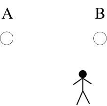
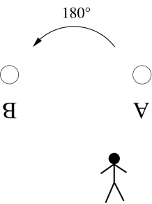
Figure 7: The presence/existence of the observer breaks the symmetry of the physical configuration under 180⁰ rotation.

Figure 8: The observer does not rotate. Now the rotated situation is not equivalent to the previous one.

There is therefore a choice which corresponds to the maximum of entropy. The real situation can be schematically depicted as follows. The “empty space” is something like in figure 9, in which the two dots, distinguished by the shadowing, represent the observer, i.e. not only “the person who observes”, but more crucially “the object (person or device) which can distinguish between configurations”.

Figure 9: The presence of an observer able to detect a motion according to a group action is something that breaks the symmetry of the Universe under this group, otherwise the action would not be detectable. Here we represent the observer as something that distinguishes A from B.

Now we add the experiment, figure 10. In this case, the previous figures 6 and 6 correspond to figures 12 and 12.

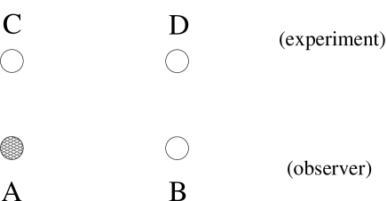
Figure 10: In the presence of an observer, here represented by the points A and B, even with a “symmetric” system, the points C, D, the Universe is no more symmetric. Points C and D can be identified, by saying that C is the one closer to A, D the one closer to B.

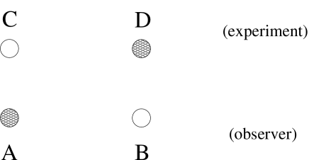
Figure 11: The analogous of figure 6 in the presence of an observer.

Figure 12: The analogous of figure 6 in the presence of an observer.

It should be clear that entropy in the configuration of figure 12 is not the same as in the configuration of figure 12. This means that the observer “breaks the symmetries” in the Universe, it decides that this one, namely figure 9, is the actual configuration of the Universe, i.e. the one contributing with the highest weight to the appearance of the Universe, while the one obtained by exchanging A and B is not.

The observer is itself part of the Universe, and the symmetric situation of the ideal problem of the double slit is only an abstraction. In our approach, it is the very presence of an observer, i.e. of an asymmetrical configuration of space geometry, what removes the degeneracy of the physical configurations, thereby solving the paradox of equivalent probabilities of ordinary quantum mechanics. In this perspective there are indeed no “probabilities” at all: the Universe is the superposition of configurations in the same sense as wave packets are superpositions of elementary (e.g. plane) waves; real waves, not “probability wave functions”. This means also that mean values, given by 2.35, are sufficiently “picked”, so that the Universe doesn’t look so “fuzzy”, as it would if rather different configurations contributed with a similar weight. Indeed, the fuzziness due to a small change in the configuration, leading to a smearing out of the energy/curvature distribution around a space region, corresponds to the Heisenberg’s uncertainty, section 3. The two points on the target plate correspond to a deeply distinguished asset of the energy distribution, the curvature of space, whose distinction is well above the Heisenberg’s uncertainty.

When objects, i.e. special configurations of space and curvature, are disentangled beyond the “Heisenberg’s scale”, “randomness” and “unpredictability” are rather a matter of the infinite number of variables/degrees of freedom which concur to determine a configuration, i.e., seen from a dynamical point of view, “the path of mean configurations”, their time evolution. In itself, this Universe is though deterministic. Or, to better say, “determined”. “Determined” is a better expression, because the Universe at time $N^{\prime}\sim{\cal T}^{\prime}={\cal T}+\delta{\cal T}\sim N+1$ cannot be obtained by running forward the configurations at time $N\sim{\cal T}$. The Universe at time ${\cal T}+\delta{\cal T}$ is not the “continuation”, obtained through equations of motion, of the configuration at time ${\cal T}$; it is given by the weighted sum of all the configurations at time ${\cal T}+\delta{\cal T}$, as the universe at time ${\cal T}$ was given by the weighted sum of all the configurations at time ${\cal T}$. In the large $N$ limit, we can speak of “continuous time evolution” only in the sense that for a small change of time, the dominant configurations correspond to distributions of geometries that don’t differ that much from those at previous time. With a certain approximation we can therefore speak of evolution in the ordinary sense of (differential, or difference) time equations. Strictly speaking, however, initial conditions don’t determine the future.

Being able to predict the details of an event, such as for instance the precise position each electron will hit on the plate, and in which sequence, requires to know the function “entropy” for an infinite number of configurations, corresponding to any space dimensionality at fixed ${\cal T}\approx N$, for any time ${\cal T}$ the experiment runs on. Clearly, no computer or human being can do that. If on the other hand we content ourselves with an approximate predictive power, we can roughly reduce physical situations to certain ideal schemes, such as for instance “the symmetric double slit” problem. Of course, from a theoretical point of view we lose the possibility of predicting the position the first electron will hit the target (something anyway practically impossible to do), but we gain, at the price of introducing symmetries and therefore also concepts like “probability amplitudes”, the capability of predicting with a good degree of precision the shape an entire beam of electrons will draw on the plate. We give up with the “shortest scale”, and we concern ourselves only with an “intermediate scale”, larger than the point-like one, shorter than the full history of the Universe itself. The interference pattern arises as the dominant mean configuration, as seen through the rough lens of this “intermediate” scale.

5 String Theory

Till now, we have spoken of “light rays”, “gravitational fields”, radius, curvature, in one word we have made an extensive use of the language of geometry and field theory, in order to make more concrete the discussion, but, despite of the language, we have always worked in a discrete formulation of the combinatoric problem. Indeed, for $N$ sufficiently large, it is not only possible but convenient to map to a continuous description, in that this not only makes things easier from a computational point of view, but also better corresponds to the way the physical world shows up to us, or, more precisely, to the interpretation we are used to give of it.

If we want to pass to a description in terms of continuous variables, we must introduce a “length” to use as a measure: in the continuum, lengths must be measured in terms of a given unit. Differently from the discrete formulation, in which all quantities: the extension of space, the amount of “energy”, the “time”, could be measured in terms of “number of cells”, in the continuum we must a priori introduce a distinguished unit of measure for any type of measurable quantity. To start with, we must introduce a unit of length, that we call $\ell$. This not only serves as a measure, but it can be chosen to coincide with the elementary size, the radius of the unit cell. In this way, we introduce what we call the “Planck length”, $\ell_{\rm Pl}$.

Energies and momenta are conjugate to space lengths, relation 2.31, and the natural unit in which they are measured is the inverse of the Planck length. This leads to the introduction of the Planck Mass $m_{\rm Pl}$ and the unit of conversion between the energy/momentum and space/time scale, the Planck constant $\hbar$ according to the relation:

$$\left[E,P\right]\,\sim\,{1\over\left[R,t\right]}~{}\leadsto~{}m_{\rm Pl}\,\stackrel{{\scriptstyle\rm def}}{{\equiv}}\,{\hbar\over\ell_{\rm Pl}}\,.$$ (5.44)

This corresponds to the usual relation between these quantities, apart from the fact that here doesn’t appear any power of the “speed of light”. In fact, till now we have paired the concepts of energy/momentum/mass because we have not yet distinguished the unit of measure of time from the one of space. Indeed, were all the objects either massless, or permanently at rest, this distinction would be unnecessary. We need to disentangle time from space in order to measure the rate of expansion of objects, “inhomogeneities” in the average geometry of space, as compared to the rate of the expansion of the space itself. As discussed, non-trivial massive objects correspond to subregions that spread out at particular rates, giving therefore rise to a full spectrum of non-trivial “speeds”. We measure these speeds in terms of $c$, the rate of expansion of the radius of the three-sphere with respect to $N$, intended as the time. In section 7.5.2 we will discuss how this can be identified with the “speed of light in the vacuum”. Obviously, the formulation in terms of discrete numbers and combinatorics corresponds to a choice of units for which all these “fundamental constants” are 1.

From the perspective of a theory on the continuum, in themselves these scales could be considered as free parameters. One could think to be forced to introduce them as regulators, but that in principle they are free to take any possible value. However, being $\ell$ the unit in which the length of space is measured, by varying it one varies the “unit of volume”, or equivalently “the size of the point”, $v$. When considering the full span of volumes $V$ we obtain a series of equivalent sets describing the same system, equivalent histories of the Universe. Running in the set $\{V/v\}$ by letting both $V$ and $v$ take any possible value results in a redundancy reproducing an infinite number of times the same situation. Similar arguments hold for the Planck constant $\hbar$ and the speed of expansion $c$. In particular, fixing the speed of expansion to a constant $c$ allows to establish a bijective map between the time $t$ and the volume $V$ of the three-spheres. Varying the map $t\to V$ through a change of $c$ would lead to an over-counting in the “history of the Universe” . In summary, we would have classes of Universes, parametrized by the values of $c$ and $\ell_{\rm Pl}$. The real, effective phase space is therefore the coset:

$$[{\rm eff.~{}phase~{}space}]\,=\,[{\rm phase~{}space}]\Big{/}\{c\},\{\ell_{\rm Pl}\}\,,$$ (5.45)

and, more in general:

$$[{\rm eff.~{}phase~{}space}]\,=\,[{\rm phase~{}space}]\Big{/}\{{\rm symmetries}\}\,.$$ (5.46)

When passing to the continuum, at large $N$, we must therefore look for a mapping of the combinatoric problem to a description in terms of continuous geometry, which i) contains as built-in the notion of minimal length, finite speed of propagation of informations, i.e. locality of physics, in which ii) energies are related to space extensions through relations such as 2.31, and in which iii) the “evolution” is labelled through a correspondence between configurations and a parameter that we call “time”. Through the relation between this parameter and the curvature, or the “radius” of the maximally entropic configurations, this parameter too can be viewed as a coordinate. Measuring also time in terms of unit cells, the same units we use to measure the space, corresponds to fixing the “speed of expansion” to 1 (later on we will see how this can be seen as the “speed of light”).

In section 4 we discussed how, for the practical purpose of reducing the combinatoric problem of the configuration of the Universe to a “humanly solvable” level, it is somehow necessary to introduce simplifications, which lead, up to a certain extent, to some degree of indeterminacy. String Theory arises as one such an approach to the problem: it is a way of representing a theory in which the minimal length is not zero, the “point” has size $\ell_{\rm Pl}$, and whose “space-time” indeed possesses a “time coordinate”, which appears built-in, although singled out from the other coordinates by a Minkowskian choice of signature of the metric. To be more precise, the Planck length is the length of the “duality invariant, unified” string theory, otherwise also called “M-theory”. The single perturbative string constructions have their own “minimal length” $\ell_{s}$, differently related to $\ell_{\rm Pl}$, according to the size and configuration of the slice of the string space they correspond to. Quantization of the string modes, in terms of raising and lowering operators, realizes a viable implementation of the quantum, probabilistic approximation of the description of physical phenomena, as discussed in the previous section. In practice, it reduces to a geometric problem the “central” value of observables, while implementing through quantization a way of dealing with the deviations from the “classical geometric solution”, and from the definability itself of observable quantities in terms of geometry and propagating fields.

In how many dimensions should we expect to be able to construct such a theory? Relativity and locality tell us that we need spinorial and vectorial degrees of freedom. Namely, that we must build the space as a spinorial space. If we want to describe the corresponding degrees of freedom through a fiber of “extra” vectorial coordinates, we need therefore twice as many coordinates as the dimensions of the space. We have seen that the dominant configuration of space is three. This is related to a specific choice of the scaling of energy $\sim N$ as compared to the scaling of space, which appeared as the natural one. String theory is built as a geometric theory endowed with a quantization principle, which implements the Heisenberg’s Uncertainty Relations, under which all “non-dominant” configurations are “covered”. In our set up, the space/momentum and/or time/energy relations appear as in the Heisenberg’s inequalities. We expect therefore that quantum string theory should be non-anomalous when built out of a number of coordinates which allows a correspondence of these descriptions.

Let’s clarify this point. On the “combinatoric side” we “center” the theory around three dimensions, that indeed are 3+1, because to the three of space we must add the time, or equivalently, the curvature. Correspondingly, quantum string theory should be something that needs 12 coordinates for its complete description. However, one of these should be a “curvature”. Projecting on a flat limit should allow a description in terms of 11 coordinates. Indeed, a perturbative description would require to single out one of these coordinates, to be used as the parameter, the “coupling” around which to expand. In practice, we should expect to be able to construct a perturbative slice of such a geometric representation of our combinatoric problem with 10 space-time coordinates. This should be the dimension in which the theory is perturbatively non-anomalous. Indeed, this is the critical dimension of perturbative superstring theory. Supersymmetry is needed in order to perturbatively introduce spinors besides vectors . However, on the combinatoric side, three space dimensions are only the “dominant” choice. On the string side, this appears as the necessary dimensionality of the “base” only once this is put in relation to the Uncertainty Relations. Namely, this procedure encodes a choice of “starting point” for the approximation of the configurations, three space dimensions, plus a rule implementing the ignorance due to neglecting the rest, the Uncertainty Relations. In this way, it is only upon quantization that string theory shows out an anomaly when built on other numbers of coordinates. Alternatively, one could think to choose a different relation between “energy” $N$ and radius, or time. We would then get a different uncertainty relation, of the type:

$$(\Delta X)^{\alpha}\Delta p\,\geq\,{1\over 2}\hbar\,,$$ (5.47)

where $\alpha$ is an exponent, $\alpha\neq 1$. In this case, quantum string theory would be non-anomalous in a different number of dimensions.

Our argument is not a proof that the critical dimension of the superstring is 10. It gives however the flavour of why it is so. Indeed, there are several things that don’t match, between our combinatoric problem and superstring as it is defined in its basic construction. First of all, in our problem time is a coordinate that labels classes of configurations, with a combinatoric the more and more complex as time increases. As it is built, superstring theory appears instead to possess a symmetry under time reversal. Moreover, string theory appears to possess an infinite number of degrees of freedom, and this not only, obviously, in the non-compact case, but also when all the coordinates are compactified. Even in this case the string spectrum contains an infinite tower of energy/momentum states, obtained both as Kaluza Klein momenta or windings. This however is not completely unexpected: a perturbative construction is built on a flattened space. What we are doing is therefore approximating the true, curved space through a series of “plane waves” in a basically non-compact space. The matching of string time and physical time is achieved once the string space is fully compactified and the redundancy produced by the scale invariance removed by the introduction of masses. In this configuration, also the symmetry under time reversal is broken (see Ref. [1]).

In our set up we have geometries of coordinates, characterized by the (local) value of the curvature, and, under certain circumstances, we can recognize a path through sets of geometries/configurations, that as discussed we interpret as a time evolution. Energies and fields belong to our interpretation of this “evolving set of geometries”: they parametrize the moving sources of geometry and curvature, and the traditional expansion in terms of harmonic excitations parametrizes the modes of the evolving shape of space. Under certain respects, these statements may sound trivial, and, after Einstein’s General Relativity, they are, either explicitly or implicitly, familiar. Nevertheless I think it is good to stress this point. From this point of view, the entire description in terms of quantum fields is a description of (a subset of) the evolving geometries of the Universe.

The combinatoric description of the universe and its string representation differ in many respects, due to the fact that the latter gives a field theoretical interpretation and implementation of discrete configurations. In the combinatoric problem, that, we underline, is the fundamental formulation of the problem, we have only “size-one” energies. Lower energies result only through averaging over longer times (or space intervals). On the string side we have on the other hand excitations that correspond to different energies; after the identification of the unit length with the Planck length, we can recognize that string theory smoothes down, averages over sets of discrete configurations: in particular, all the sub-Planckian string excitations correspond to collections of discrete configurations. Energies (and momenta) of the compactified string are however built not only over a basis of Kaluza Klein modes:

$$E_{m}\,\sim\,{m\over R}\,,$$ (5.48)

where $R$ is a compactification radius, but also as “winding” modes:

$$E_{n}\,\sim\,{nR}\,.$$ (5.49)

These are normally introduced in toroidally compactified perturbative string vacua, where lengths are measured in terms of the appropriate string length $\ell_{s}$ (as we said, each perturbative string construction has its own proper length; this is an artifact of the representation of the whole theory through a set of perturbative slices). However, we can already by now say that, in the cases of interest for us, namely for the string configurations that dominate in the phase space, the proper string length and the Planck length can be identified . Under identification of the string length with the Planck length, $\ell_{s}=\ell_{\rm Pl}$, we can view the first Kaluza Klein excitations of 5.48, namely those with $m<R$, as the sub-Planckian ones. As we have seen in section 3, the contribution of all the possible configurations at any time is “contained” in the uncertainty corresponding to the Heisenberg’s principle. At any time the various configurations contribute and give origin to a spreading-out of the unit values of energies, producing a varied spectrum, that only in the “average”, and up to the Heisenberg’s bound, corresponds to a three-sphere. Saying “in the average” precisely means that a three-sphere is rigorously only the very maximal entropy configuration, while the non-maximal ones contribute by spreading out mean values according to the Heisenberg’s relations . Accounting in its spectrum for mass excitations lower than the Planck scale, and coming with an endowed “quantization principle” through (anti)-commutators etc…, string theory collects therefore in one “averaged” description the effect of a superposition of configurations of maximal and “close-to-maximal entropy”. As discussed in [1], string vacua describe massive excitations through a superposition of plane waves living on spaces with shorter radius than the whole three-dimensional space. They are therefore “localised” objects; indeed, as we have discussed in section 2.4, these “wave packets” are short-extension inhomogeneities of the geometry. We will come back to this point, with a discussion of both the string and the combinatoric point of view, in sections 6.6, 6.7.

5.1 T-duality

The winding modes 5.49 can be viewed as the Kaluza Klein modes built over the so-called “T-dual” radius, $\tilde{R}=1/R$, somehow enabling to introduce in the game also lengths “shorter” than the minimal one, $\ell_{s}=\ell_{\rm Pl}$. The existence of a minimal length is assured in string theory by the existence of a symmetry, called T-duality, of the compactified string, that basically maps energy excitations built as Kaluza Klein momenta over length scales below the string length to dual excitations built as windings, in practice Kaluza Klein momenta over the inverse scale. So, once reached the string length, the system “bounces” back above this scale. We already pointed out that, in order to concretely “solve” the combinatoric problem of the physical world, it is useful to think in terms of symmetries, and eventually discuss how and how much these symmetries are broken or up to what extent preserved. This is somehow unavoidable. The toroidally compactified string, with its symmetry under T-duality, is an example of such a theoretical “simplification” of the true physical situation, which allows to reduce the amount of degrees of freedom. Seen in this way, T-duality appears as a convenient description; there is nothing particularly fundamental in it from a physical point of view: fundamental is the regularization of the phase space through the introduction of a minimal length, a property of which string theory provides an implementation. T-duality is eventually softly broken in the very dominant vacuum [1]. Nevertheless, it turns out to be convenient to parametrize physics in terms of strings and T-duality, namely by first introducing a strong simplification via string theory on a compact space, in which T-duality is a way of introducing a regulator; the real world is then better approximated by softly breaking this symmetry.

Thinking in terms of T-duality and string theory allows to work around a vacuum that we can keep under control. Through this approach, we have access to some relevant properties of the dominant configurations of the Universe, which can in this way be viewed as a soft perturbation of a “simple” vacuum. For instance, in this way we know what are the terms necessary to keep it non-anomalous, and therefore what is the configuration that does not generate an uncontrolled, possibly infinite number of terms, something that would correspond to generate “new dimensions” and lead to a configuration more entropic than expected. E.g. we know that we must work in 10 dimensions and not in 8 or 14 etc… But for the real physical world there is no “softly broken T-duality”.

6 Macroscopical and microscopical entropy

In its basic construction, superstring theory appears embedded in a non-compact space. In particular, the time coordinate appears to be allowed to span over the infinite real axis without constraints. On the other hand, we already remarked that any perturbative construction implicitly corresponds to some decompactification limit. As we discussed in sections 2.1 and 2.8, the number of “cells” of the target space of our combinatoric problem, what we called the “volume” $V$, is arbitrarily large, something we indicate by saying that we take the limit $V\to\infty$. This however does not mean that what we call “space” in the ordinary sense is at any (finite) time infinitely extended. Indeed, cells without an assigned geometry have no intrinsic meaning as a space in our ordinary sense: it is only after we have assigned a geometric interpretation that we give them also such a meaning. In particular, we have seen that the configuration of the universe at any finite time in the average classically corresponds to a three-sphere of radius $N=(c){\cal T}$, the light-equivalent of the age of the universe. At any finite time we see all the volume $V$, but configurations that depart from the average one of radius $c{\cal T}$ appear as perturbations of the mean geometry, which are not all interpretable in geometric terms. As we have discussed, they all fall under the “cover” of the Uncertainty Principle, and are related to what we interpret as the quantum nature of physical phenomena. In other words, this is like to say that at any time ${\cal T}$ we indeed do see the entire space, but this can be reduced to the ordinary geometric interpretation of space only up to a distance $c{\cal T}$, i.e. as long as classical light rays have carried to us the information about it.

• Only up to $R=c{\cal T}$ such a “whole” can be interpreted according to our “classical” concept of space, which cannot be disentangled from time, because we “see” space only through light rays coming to us.

Our perception of space is produced by light rays that come to us travelling in space-time.

• The space “outside” the horizon is certainly infinitely extended, and somehow we see it, but it contributes to our perception and measurements only for an “uncertainty” of mean values, accounted for by the Heisenberg’s uncertainties.

From a classical point of view, at any finite time ${\cal T}$ space exists only up to $R=c{\cal T}$. From this point of view, namely from the point of view of writing a theory in terms of differential geometry, at finite time the space is always compact, of finite volume.

In order to represent a mapping of our combinatoric problem at any finite time, we must therefore consider also string theory on a compact space. This implies that it must be considered in a non-perturbative regime, where in particular, owing to compactness of the space, supersymmetry is broken. In order to understand then what kind of “universe” comes out of all the possible configurations, or “string vacua”, at any fixed volume, we must find out those that correspond to the maximal entropy in the phase space. String configurations on a compact space are obtained by compactifying the string target space on certain spaces, which may be continuous and differentiable, or even singular. In any case, a compactification leads to a reduction of the symmetry of the initial theory. The more singular is the space on which the string is compactified, the higher is the amount of symmetry reduction. The spectrum of “massless states” is related to the surviving symmetries of the target space. By considering not just the massless states, but the full string spectrum, it is easy to see that the more the target space is “singularised”, the more “diversified” is the spectrum one obtains, as a consequence of the symmetry reduction, and the higher is also the number of possibilities such a configuration has of being realized in the phase space.

A way of constructing configurations is to divide the string space through the action of a symmetry group. The method of obtaining configurations by taking a quotient is typical of string constructions, not only in the case of orbifolds, where one mods out by a discrete symmetry; also in the case of Calabi Yau constructions or generic compactifications, the “massless” degrees of freedom are related to the surviving (continuous) deformations of the compact space. In that case, we can at least formally say that one mods out by a continuous symmetry.

Let’s consider the action of a group $Q$, and consider the configuration $\Psi$ obtained by dividing the string space by $Q$. The volume $V$ of the phase space of the initial configuration gets divided into cells of volume:

$${\rm v}\,=\,{V\over Q}\,.$$ (6.50)

The configuration $\psi$ occupies one of these cells. Let’s say it is supported on ${\rm v}$. Elements $q,q^{\prime}\in Q$ map the cell/sub-volume ${\rm v}$ to equivalent cells/sub-volumes, as illustrated in figure 13.

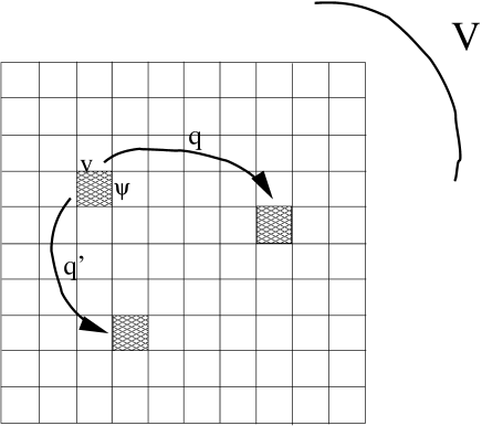
Figure 13: The configuration $\Psi$, occupying a volume ${\rm v}$ in the initial phase space of total volume $V$, is mapped to equivalent sub-volumes by the action of the elements $q$ of a symmetry group $Q$, $q,q^{\prime}\in Q$.

There are therefore $Q=V/{\rm v}$ ways of realizing this configuration. The occupation in the whole phase space is therefore enhanced by a factor $Q$ as compared to the initial one. By reducing the symmetry, we have enhanced the possibilities of realizing a configuration in equivalent ways, in the same sense as, in the two-cells example of section 2, by assigning different colours, black and white, we have the possibility of realizing the configuration “one-white/one-black” in more ways than “white-white” or “black-black”.

6.1 Microscopical entropy

The entropy considered in section 2, given as the logarithm of the occupation in the phase space of all the combinatorics at given volume, can be considered the “macroscopical entropy” of the space of all possible configurations of degrees of freedom in a certain volume. This is directly related to the weight of the contribution of a certain configuration to the way the Universe appears. The higher is entropy, the more a configuration contributes, as it should. On the other hand, one can consider each configuration as a “universe” in itself. There is a “string partition function”, built over a bunch of states, the states of the string spectrum. These states contribute to the string partition function with weights that can be related to their probability in the specific string vacuum they belong to. It is therefore possible to speak of a “microscopical entropy”, the entropy of the specific “gas of states” which contribute to create the “geometry” of a string vacuum. In turn, each string vacuum can be viewed as belonging to a “gas of spaces”, where the macroscopical entropy is defined. It turns out that the two entropies are “dual” to each other: the microscopical entropy decreases as the distribution of states of a single vacuum is more concentrated; this means that the symmetry of this vacuum is highly reduced, and in turn the occupation of the whole configuration in the full phase space is enhanced. Let’s consider the effect of a symmetry reduction on the occupation volume, the “weight” $W$ of a configuration. Let’s suppose we start with a symmetry $Q$. Let’s now enhance/reduce, at fixed volume, the symmetry of the configuration to $Q^{\prime}$, such that the volume $||Q^{\prime}||$ of the group $Q^{\prime}$ is $\alpha$ times the volume of the group $Q$: $||Q^{\prime}||=\alpha||Q||$, something that we shortly indicate as $\alpha:Q\to\alpha Q$, using the same notation for the volume factor $\alpha$ and the operator $\alpha$ that performs the transformation from one group to the other one. The weight of the configuration in the full phase space behaves as a homogeneous function of the symmetry factor, of degree 1:

$$Q\,\to\,\alpha Q\,,~{}~{}\Rightarrow\,W_{\rm macro}(Q)\,\to\,W_{\rm macro}(\alpha Q)\,=\,\alpha W_{\rm macro}(Q)\,.$$ (6.51)

On the other hand, at the microscopical level, the weight is a homogeneous function of degree -1:

$$W_{\rm micro}(Q)\,\to\,W_{\rm micro}(\alpha Q)\,=\,\alpha^{-1}W_{\rm micro}(Q)\,.$$ (6.52)

This, for any fixed volume $M$. We can therefore write:

$$W_{\rm macro} = A(M)\,Q\,;$$

$$W_{\rm micro} = B(M)\,Q^{-1}\,.$$

Writing $W_{\rm macro}=\exp S_{\rm macro}$, $W_{\rm micro}=\exp S_{\rm micro}$, we obtain that:

$$S_{\rm macro}\,=\,-S_{\rm micro}\,+\,F(M)\,,$$ (6.54)

where $F(M)=\ln\left(A/B(M)\right)$. The entropy considered in Ref. [1] is precisely the microscopical entropy, $S_{\rm micro}$. Indeed, while in the macroscopical picture we work “at fixed energy $N$”, in the microscopical one we classify the ordering through “space” volumes $M\geq N$. In order to derive the dominant configuration of the universe, in the macroscopical picture we look for the highest entropy at fixed energy $N$, in the microscopical one at the minimal entropy at fixed volume. The two approaches are dual to each other. The “macro” picture is the picture of energies, the “micro” one is the picture of space volumes, namely of the size of the space of the space-coordinates. Indeed, the two “coordinates” are conjugates each other; this somehow reflects the Uncertainty Relation(s):

$$\Delta E,\,p~{}~{}{\displaystyle{{\raise-8.0pt\hbox{$>$}}\atop{\raise 5.0pt\hbox{$\sim$}}}}~{}~{}{1\over\Delta t,\,X}\,.$$ (6.55)

These relations are “symmetric” in energies (i.e. attributes) and space-time. In one picture, we fix the attributes and have an uncertainty in the size of space-time. In the other one, we fix the size of space(-time) and have an uncertainty in the energies.

If we work at fixed $M$ (“fixed volume” in the language of [1]) we can neglect the additive constant $F(M)$, that in this case results in a multiplicative rescaling of all the weights, irrelevant to the purpose of computing mean values of observables. We recover therefore the relation of Ref. [1], expressing the weight of a configuration at a given volume as:

$$W(\Psi)_{V}\,=\,{\rm e}^{-S\,(\equiv S_{\rm micro})(\Psi)}\,.$$ (6.56)

Notice that $A(1)=B(1)$, implying that $F(N=1)$ vanishes: the macroscopical and microscopical weight meet at $N=1$, where there is only one possible configuration, in both the macroscopical and the microscopical sense (this is however a limit case well beyond the regime of validity of the string approximation).

As it is written, $S_{\rm micro}$ appears to be the mapping of the weight of a configuration to the “tangent space”. As discussed in Ref. [1], this logarithmic representation of space is the environment in which perturbative string is normally constructed, and operations such as the orbifold projections naturally defined. This is the reason why, as discussed in [1], $Z_{2}$ orbifold shifts, introducing $1/2$ projections on the tangent space, and therefore on the occupation volumes in the logarithmic representations, lead to square-root scalings of physical masses. Logarithmic masses are related to the microscopical entropy, as well as physical masses are related to the occupation volume in the “pulled-back”, real space.

6.2 Mean values and observables in the string picture

Since expression 2.35 is normalized, any difference in the normalization of the macroscopical and microscopical definitions of entropy, eq. 6.54, becomes irrelevant. Expression 2.35 is therefore valid both at the discrete level, for the combinatoric problem of the full phase space, and at the “microscopic level” of those particular subsystems, “collections of macroscopic configurations”, which are the string vacua. In the first case, the weight $W(\Psi)$ of a configuration is given by:

$$W(\Psi)\,\stackrel{{\scriptstyle\rm def}}{{=}}\,\exp S_{\rm macro}(\Psi)\,,$$ (6.57)

where $S_{\rm macro}$ is the entropy of the configuration in the full phase space. In the second case,

$$W(\Psi)\,\propto\,\exp-S_{\rm micro}(\Psi)\,,$$ (6.58)

where $S_{\rm micro}$ is the entropy of the states within each string vacuum, and the symbol “$\propto$” can be substituted by “$=$”, as long as the final scope is that of computing mean values. Analogously, the partition function ${\cal Z}$ admits the two corresponding interpretations. Notice that on the string side the partition function ${\cal Z}$ can be normalized only when the space is compact, and therefore curved, with a non-vanishing curvature due to the fact that we work at finite volume. Any perturbative construction is built on a non-compact space, and somehow corresponds to the limit $N\to\infty$. In the orbifold language, the condition of working in a curved, compact space is attained at the maximal twisting [1]. Nevertheless, one can built vacua with a non-vanishing partition function by explicitly breaking supersymmetry .

According to 6.57, 2.35 receives contributions mostly from the configurations with the highest macro (resp. lowest micro) entropy. One may ask what happens if ${\cal O}$ diverges on some non-extremal entropy configuration. In this case, the main contribution to the mean value of the observed quantity could come from seemingly negligible vacua. This however is a wrong way of approaching the problem, a way of thinking that makes only sense in the traditional approach of observable quantities defined in terms of operators acting on an effective action, written as an explicit function of terms determining the dynamics of the system. In this approach, physical quantities such as masses, energies, couplings have a value, a “weight” depending on their occupation in the phase space: particles that interact more are heavier etc…, as discussed in [1]. Owing to their very basic definition, observables cannot “blow up” on rare configurations: they acquire a non-negligible contribution from their being in correspondence with (relatively) often realized processes (see discussion in Ref. [1]).

6.3 Entropy and curvature

In Ref. [1] we discussed how, upon sufficient “singularization”, the string vacuum becomes necessarily curved, with an entropy equivalent to the one of a three-dimensional black hole: $S\sim{\cal T}^{2}$, where ${\cal T}$ is the age, or equivalently the radius, of the Universe. On the other hand, we also observed that, in principle, string theory on a compact space is always embedded in a curved space. However, a perturbative construction is forcedly build around a de-compactification limit of some coordinates, contributing to the definition of what is considered the “coupling” of the theory. In string perturbation it is therefore possible to work with supersymmetric vacua and flat spaces. The string representation of the geometric/combinatoric problem we are discussing in this work is somehow a mapping, in which the degrees of freedom describing the geometries of space and their evolution are represented in terms of coordinates of a fibered space, “folded out” in a flat representation, that corresponds to a logarithmic, “tangent space” description. String theory “lives” on a fibered space that parametrizes in terms of fields and waves the combinatoric problem, which is a problem in itself entirely related to the physical space-time. In other words, with string theory we build-up an extra space, a fiber over the physical space, in order to parametrize in a continuous way the combinatorics of the geometry of the space. The “macroscopic” curved geometry results from a process of singularization of this “folded out” space, obtained e.g. through progressive orbifolding. Let’s consider for instance the probabilities of the states as they appear in the string (one loop) partition function, once the space is sufficiently curved to make the latter non-vanishing and therefore the probabilities normalizable:

$$P\,\cong\,{\int d\tau\,{\rm e}^{-E^{2}\tau}\over{\cal Z}}\,\to~{}\approx{1\over E^{2}}\,{\cal Z}^{-1}\,.$$ (6.59)

Compare this expression with the usual definition of probability for a statistical system at equilibrium:

$$P\,=\,{{\rm e}^{-\beta E}\over{\cal Z}}\,.$$ (6.60)

A comparison of these expressions clearly suggests that the string (perturbative) partition function is defined on the logarithm, on the tangent space.

Entropy reduction is obtained through compactification of the string target space on more and more curved geometries. Spaces with higher curvature have in fact a smaller symmetry group. In Ref. [1] we have described this process in terms of orbifold projections. Before attaining the maximal twisting of string vacua, we analyse entropy only in perturbative slices of the string theory (at maximal twisting, the vacuum is necessarily non-perturbative because no decompactification limit can be taken). On these slices, we have a partial view of the story, and we can work on a compact subset of the full string space. There, we can apply projections that reduce entropy. This corresponds to focusing on a subset of “coordinates”, of which we can fix the (sub)volume, ignoring the fact that other coordinates are non-compact. We control therefore the reduction of entropy separately on the various slices that patch together to build up the string vacuum.

In Ref. [1] we have discussed how orbifolds are the privileged constructions for following the process of entropy reduction in string theory. In order to understand how the reduction works, we can figure out the situation by representing the initial physical system as a gas of identical particles. We quote here the discussion presented in Ref. [1].

A string vacuum (and in particular an orbifold) can be thought as a gas, in which different particles act as sources for the singularities of the space (from a gravitational point of view, particles are singularities of space-time, being sources of gravitational field, singular points of the curvature). Let’s consider the case of a $Z_{2}$ orbifold. The orbifold projection introduces a “distinction mark” on half of the states, it labels them in another way. The situation is depicted in figure 14.

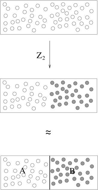
Figure 14: the effect of an orbifold projection is that of reducing the symmetry of the system, separating the spectrum in two sectors “confined” to different parts of the phase space.

The resulting orbifold follows now the laws of the composite systems: the probability of the various configurations of the new string “vacuum” are given by the product of the probability of the unprojected part (“A” in figure 14) times the probability of the twisted part (“B” in figure 14):

$$P_{A+B}~{}=~{}P_{A}\times P_{B}\,.$$ (6.61)

Let’s assume we know the entropy of the string vacuum before the orbifold projection. We want to see how this quantity changes when we apply the $Z_{2}$ projection. Intuitively, it is clear that, since a projection reduces the amount of symmetry, it reduces also the volume of the phase space at disposal for the degrees of freedom. As a consequence of the increased concentration of the probability distribution, we expect that also entropy should be reduced. In order to see more precisely how things work, consider that a $Z_{2}$ projection divides the initial system in two parts, as is clear from the partition function:

$${\cal Z}~{}\stackrel{{\scriptstyle Z_{2}}}{{\longrightarrow}}~{}{1\over 2}\left({\cal Z}{0\atopwithdelims[ ]0}\,+\,{\cal Z}{0\atopwithdelims[ ]1}\right)\,+\,{1\over 2}\left({\cal Z}{1\atopwithdelims[ ]0}\,+\,{\cal Z}{1\atopwithdelims[ ]1}\right)\,.$$ (6.62)

This corresponds to the process illustrated in figure 14. In order to understand in which direction the variation of entropy goes, we can view the process of separation of the phase-space into two sectors as the opposite of the adiabatic expansion illustrated in figure 15.

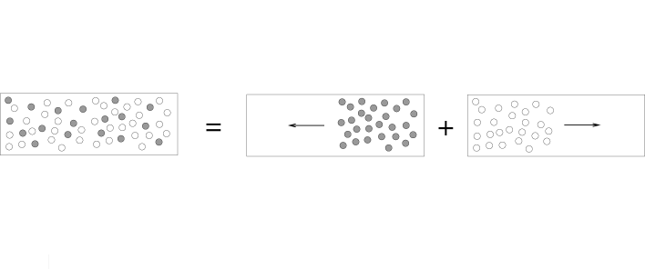
Figure 15: The entropy decrease due to an orbifold projection can be understood if we represent the system as the sum of two parts each one consisting of a gas of particles. The orbifolding process is the reverse of the expansion of each of the two gases from half of the phase space until they occupy the entire phase space.

In this example, the system is constituted by the sum of two subsystems of particles, that for convenience we have labelled with a different colour. Intrinsically, they are on the other hand indistinguishable; when they are together, such as on the l.h.s. of the figure, all particles are on the same footing, having at disposal the full phase space. Our system is the sum of the two systems on the r.h.s., and entropy is the sum of the two corresponding entropies. It is then clear that, owing to the process of “separation” induced by the orbifold operation, entropy decreases.

We can compute the amount of this reduction. Although represented as a “gas”, the system does not follow the laws of gas thermodynamics: the particles don’t have a “temperature” related to a “kinetic energy”. In order to understand what happens to entropy, we must only think in terms of phase space and probability distributions. We can consider the whole system as ideally divided into two subsystems, A and B. The probability of each half system is 1/2 of the total probability:

$$P_{A}\,=\,P_{B}\,={1\over 2}\,,$$ (6.63)

When this distinction is just virtual, as it is before the orbifold projection, the total probability of the system is $1=1/2+1/2$. As illustrated in figure 14, the $Z_{2}$ projection acts like the insertion of a wall between A and B, that prevents a mixing of the two parts. In this case, the probability of the configuration “A B” is the product of the two probabilities, because the phase space too has become a product:

$$P_{AB}\,=\,P_{A}\times P_{B}\,=\,{1\over 2}\times{1\over 2}\,=\,{1\over 4}\,.$$ (6.64)

Entropy of the initial system $S_{A+B}$ is given by the sum $S_{A}\,+\,S_{B}$:

$$S_{A+B}~{}=~{}2\,S_{A}~{}=~{}\ln 2\,.$$ (6.65)

After the projection, we have instead:

$$S_{AB}~{}=~{}-P_{A}P_{B}\ln P_{A}P_{B}~{}=~{}{1\over 2}\ln 2\,.$$ (6.66)

Entropy is therefore reduced by half.

This example suggests that it should be possible to translate the problem of entropy minimization in the string configurations into geometric terms. The single particles of the gas can in fact be viewed as sources of singularity for the geometry. The less entropic configurations are also the more singular ones from a geometric point of view. Let’s introduce the “normalized curvature” $\rho(R)$:

$$\rho(R)_{\vec{x}}\,\stackrel{{\scriptstyle\rm def}}{{=}}\,{R(\vec{x})\over\int dV\,R(\vec{x})}\,.$$ (6.67)

Like a probability, this “density of curvature” sums up to 1 over the entire space. Here a comment is in order. We are used to think that, being energy/masses sources for the curvature, they should scale proportionally to the curvature, as according to the Einstein’s equations. On the other hand, from 6.59 we see that the probability of the elementary states on which the string representation is built scales as the inverse squared of the energy, and not of a length: $P\sim 1/E^{2}$. This may seem contradictory with the identification of expression 6.67 with a probability density. However, perturbatively the string fibered space representing the combinatoric problem of the “geometries” of space and its evolution is built over a set of plane wave states. Any “point-like” source of singularity, the “particle”, doesn’t appear as an elementary state of the string construction: any picked energy distribution must be built as a superposition of plane waves; the more is this wave packed picked around a point, the higher is the spreading in the momenta, according to the Heisenberg’s relation of space-momentum uncertainty, $\Delta X\Delta P\geq\hbar/2$. The “point-like” sources are build as superpositions of plane waves. This implies that a high $\rho(R)_{\vec{x}}$ is spread over also low values of $E^{2}$. Curvature and energy are therefore somehow reciprocal: ${\rm Energy}^{-2}\leftrightarrow\approx\rho(R)$. A high curvature density means that the superposition of waves contains excitations that range from low to high energy. Owing to the reciprocal relation of space and energy spreading (the Heisenberg’s uncertainty relation), also point-like and wave-like representations are somehow “reciprocal”: for what matters a representation in terms of these elementary states, energy is here equivalent to a length, rather than to its inverse. Expression 6.67 works therefore indeed as the equivalent of a probability for the string representation of the combinatoric problem: it is defined as the probability on a geometric representation of the string space not in terms of plane waves, but of superpositions of them, building up “point-like” sources of space curvature. This allows us to introduce a new definition of entropy:

$$S\,=\,-<\rho(R)\ln\rho(R)>\,.$$ (6.68)

This expression is equivalent to the usual statistical definition:

$$S\,=\,-<P\ln P>\,,$$ (6.69)

but it better fits the representation of the string space as a geometric space. In the points in which the curvature vanishes, expression 6.68 does not diverge, because they are to be considered as attained through analytic continuation from the neighbouring regular points with non-vanishing curvature. Working with a “regularized” space, with arbitrary but finite volume $V$, and therefore a non-identically-vanishing curvature, allows us to compare entropies of any different configurations of the phase space.

example: curvature density and entropy for orbifolds

Orbifolds are constructions in which the curvature can be considered entirely concentrated on the fixed points, while the rest of the space is flat. There are formulae which allow to compute the (total) curvature of an orbifold. Were this a homogeneous space with constant curvature, we could then normalize the curvature by dividing the value of the curvature by the volume of the compact space. We would have therefore:

$$\rho(R)\,=\,{R\over VR}\,=\,{1\over V}\,.$$ (6.70)

Orbifolds can instead be viewed as limits of a regular configurations, corresponding to a space in which each fixed point $i=1,\ldots,n$ is blown up to a small sphere of volume $v_{i}$. If the full orbifold space has volume $V$, and for simplicity we use the same notation in order to indicate volume and space, we have that the full space/volume can be written as:

$$V\,=\,\left\{v_{1},\ldots\,v_{n}\right\}\cup\,\left\{V-\left\{v_{1},\ldots,v_{n}\right\}\right\}\,.$$ (6.71)

Entropy in $\left\{V-\left\{v_{1},\ldots,v_{n}\right\}\right\}$ can be computed by analytic continuation, and therefore turns out to vanish. In order to see what happens on the $n$ fixed points, consider that:

$$\sum_{i=1}^{n}v_{i}R_{i}\,=\,\int R\,dV\,.$$ (6.72)

For simplicity, we can choose $v_{i}=v_{j}=v$. We have therefore:

$$R_{i}\,=\,{\int R\,dV\over nv}\,,$$ (6.73)

from which we obtain:

$$\rho_{i}\,=\,{1\over nv}\,.$$ (6.74)

The curvature density at the fixed points should correspond to a limit regularized by subtracting infinities:

$$\rho_{i}\,=\,\lim_{v\to 0}1/v\,=\,1/n\,.$$ (6.75)

This expression corresponds to considering $v$ as the unit of measure of volumes. With this “trick” we are in the position to see how an orbifold possesses a lower entropy than a smooth manifold with constant curvature equal to the average orbifold curvature. In the orbifold case, entropy is:

$$S_{\rm orb}\,=\,-\int_{\{n\}}\rho(R)\ln\rho(R)\,=\,-\sum_{i=1}^{n}{1\over n}\ln{1\over n}\,=\,-\ln{1\over n}\,.$$ (6.76)

In the smooth case, we have instead:

$$S_{\rm smooth}\,=\,-\int_{V}\rho(R)\ln\rho(R)\,=\,-\int_{V}{1\over V}\ln{1\over V}\,=\,-\ln{1\over V}\,.$$ (6.77)

Since $\{v_{1},\ldots,v_{n}\}\subset V$, $nv<V$ and $1/V<1/n\,(=1/nv)<1$, we have $S_{\rm smooth}>S_{\rm orb}$.

The unit volume $v$ can be considered as the volume of the “point”. Indeed, we can “measure” the overall volume in units of the volume $v$ of the “elementary cell”. We already pointed out that the introduction of such an elementary unit is a necessary step for the whole set up to make sense. This allows us to compare any volume to the volume of a point. When doing the comparison, it is intended that all lengths are measured in units of the elementary length $\ell$, so that a curvature, or a segment, are measured in units of $\ell$, a $d$-dimensional volume is measured in units of $v\sim\ell^{d}$. Appropriate powers of $\ell$ also adjust densities to adimensional quantities to be inserted in logarithms or exponentials.

In Ref. [1] we have seen that through orbifoldization we can obtain a vacuum which is quite close to the dominant configuration of space-time. We have on the other hand seen that the geometry of this space is basically the one of a three-dimensional black hole. In section 2.2 we have computed the scaling of entropy in the dominant configurations: $S\sim N^{2}\leftrightarrow{\cal T}^{2}$, a result derived in Ref. [1](chapter 4) directly from the string partition function. The orbifold action on the string space was a combination of freely and non-freely acting orbifolds. The non-trivial action on the extended coordinates was freely acting. In a freely acting orbifold the curvature is not “concentrated” on fixed points: these are “shifted”, in the sense that the associated massless states are lifted in mass as a consequence of the space translation associated to the twist. We can consider that the curvature is “smeared” over “extended points”. Indeed, over the entire space, although reduced in volume. In the case of a $Z_{2}$ orbifold, on half the initial volume. In practice, entropy behaves as in 6.77, with an appropriately rescaled volume, e.g. $V\to V/2$. As a result, we obtain:

$$S_{Z_{2}-{\rm freely}}\,=\,\ln{V\over 2}\,,$$ (6.78)

instead of $\ln V$ as in 6.77. Expression 6.68 seems therefore to lead to a logarithmic scaling of entropy as a function of the coordinates, and this seems in contradiction with the main power-law scaling of the black hole. Indeed, the relation between the spheric curvature that results at the maximal twisting, and the expression of entropy as a logarithm of the curvature, is established “on the tangent space”, where the internal string space “folds out” to a product of coordinates. The contributions of twisted and extended coordinates sum up, so that the internal non-freely acting orbifold actions, contributing for terms of the type 6.76, contribute to entropy for an irrelevant additive constant. The logarithmic dependence on the volume of the extended space corresponds instead to the Jacobian of the transformation between the logarithmic representation of the coordinates, where one “builds up” the string curvature, and the physical representation of space-time. In other words, an entropy given as a logarithmic function of the volume is due to the “logarithmization” of the space of degrees of freedom, implicit in any perturbative string representation:

$$\partial r^{2}\,\stackrel{{\scriptstyle\log}}{{\longrightarrow}}\,\partial(\log r)^{2}\,=\,{\log r^{2}\over r^{2}}\,\partial r^{2}\,.$$ (6.79)

6.4 Reducing entropy

According to 6.57 and 2.35, the dominant string configurations are those of minimal entropy. A way of reducing entropy consists in freezing degrees of freedom. Indeed, this is the most effective way. Let’s see what is the variation in entropy between configurations differing by the amount of frozen coordinates, and what is the one due to a change of volume of extended coordinates. For simplicity consider a configuration of $n$ coordinates, in which $p$ coordinates are extended up to $L$, and $n-p$ are frozen to size 1 in Planck units. The total volume is:

$$V\,=\,L^{p}\,,$$ (6.80)

while the curvature, the average curvature, is:

$$R\,=\,L^{p/n}\,.$$ (6.81)

The integral of the curvature over the entire volume is therefore:

$$\int R\,dV\,=\,L^{p}\times L^{p/n}\,,$$ (6.82)

and the “normalized curvature” is:

$$\rho(R)\,=\,{1\over L^{p}}\,.$$ (6.83)

The entropy of this configuration is then:

$$S\,=\,{1\over L^{p}}\ln L^{p}\,.$$ (6.84)

The relative variations with respect to $p$ and $L$ are:

$${1\over S}{\partial S\over\partial p} = {1\over p}\left(1+{1\over\ln L^{p}}\right)\,=\,{1\over p}-\ln L\,;$$ (6.85)

$${1\over S}{\partial S\over\partial L} = -{p\over L^{p}}\left(1+{1\over\ln L^{p}}\right)\,.$$ (6.86)

Notice the opposite sign of these variations, in agreement with the fact that an increase of $p$ leads to a spreading out of the curvature, and therefore an increase of entropy, while an increase of $L$ differentiates more the extended from the reduced coordinates, producing a higher differentiation in the geometric shape of the space, and a reduction of entropy. Clearly, for $p$ sufficiently small and $L$ large enough,

$$\left|{1\over S}{\partial S\over\partial L}\right|\Big{/}\left|{1\over S}{\partial S\over\partial p}\right|\,\approx\,{1\over L^{p}}\,\ll\,1\,.$$ (6.87)

Therefore, the natural direction of the process of entropy reduction is toward a maximization of the number of “frozen” coordinates (in string-orbifold language = maximal twisting). However, as we discuss in section 7.1, there is a “bound” on the maximal “twisting”.

6.5 String in anomalous dimensions and entropy

We have seen that, by reducing the volume and the dimension of space, entropy is reduced. Thinking in this way, one should conclude that, for the string in dimension $<10$, we have a reduced entropy as a consequence of a reduced number of degrees of freedom. This is not true: the string is dimension $d<10$ is anomalous: it is consistent only if seen as the compactification of the critical string. Indeed, the anomaly generates an infinite number of (counter)-terms, which correspond to switching-on new coordinates. Alternatively, we can think of parametrizing these degrees of freedom through fields (Liouville fields); this is equivalent. How many extra coordinates do we have? As many as to reach the critical dimension. In the case of string in dimension higher than 10, the anomaly generates infinitely many terms, and there is no “fixed point”, dimension at which the game stabilizes: we generate an infinite number of dimensions.

6.6 Shifts in string theory and volume reduction in phase space

In Ref. [1] we have explained the sequence of masses of the elementary particles through the relation to their occupation in the phase space. The more a particle interacts, the more are its decay channels, the heavier it is. In particular, in order to estimate the relative occupations in the phase space, we proceeded by counting the number of “symmetry reductions” the string vacuum went through in order to give rise to a certain kind of particle. Let’s see how this works in the case of $Z_{2}$ orbifold projections. Let’s suppose we start with a certain string vacuum, in which there is a set of particles with a mass produced by a $Z_{2}$ orbifold shift on the momenta, such that $m\to m+1$. We have:

$$M\,\sim\,0\to{1\over R}\,.$$ (6.88)

Let’s act now on this set with a further $Z_{2}$ orbifold projection, that reduces the symmetry by lifting half of the previous particles with a new shift on the momenta, along another direction, compactified on a circle with equal radius as the first one:

$$M\to M^{\prime}\,\sim\,{1\over R}\,+\,{1\over R^{\prime}}\,,~{}~{}~{}~{}~{}~{}R=R^{\prime}.$$ (6.89)

We end up with a vacuum in which half of the particles have mass $1\over R$, and half have mass ${1\over R}+{1\over R}$. As discussed in [1], these operations are carried out in a logarithmic representation of the physical vacuum, so that, in the “true” space, the ratio of masses is not $M^{\prime}/M=1/2$, but $M^{\prime}=\sqrt{M}$ in Planck units.

Apart from the scaling law, linear or exponential depending on whether we work on the true space or, like in perturbation theory, “on the tangent space”, we see here how a $Z_{2}$ orbifold operation can reduce the symmetry of the vacuum and at the same time pop out a new kind of particles, corresponding to the lifting of half of the previous ones. The ratio of masses between those originating as the reduction of the pre-existing ones, and the new ones with a shifted mass, corresponds to the ratio of the “volumes” of the symmetry groups of the vacuum, inversely related to the ratio of the volumes occupied in the phase space by the two configurations. Namely, with the new projection, in the phase space there are now, among others, both the “initial” configuration $\Psi$ and the configuration $\Psi^{\prime}=Z_{2}(\Psi)$. In $\Psi$ there are only particles of mass $M$; in $\Psi^{\prime}$ one-half of the particles originate as the reduction of the old ones, one half have new attributes. The configuration $\Psi$ has twice as much symmetry volume as $\Psi^{\prime}$. In the full phase space it occurs therefore half of the times of $\Psi^{\prime}$. This means that the particles with mass $M$ occupy a fraction of phase space $V_{M}\propto 1(\Psi)+2\times{1\over 2}(\Psi)$, where ${1\over 2}(\Psi)$ is the contribution of the particles of mass $M$ belonging to $\Psi^{\prime}$. The new particles occupy instead a fraction $V_{M^{\prime}}\propto 2\times{1\over 2}(\Psi)={1\over 2}V_{M}$, and consequently have mass: $M^{\prime}=M/2$ (in the tangent space, or $M^{\prime}=\sqrt{M}$ in the exponential representation. Remember that masses are lower than 1, so that $\sqrt{M}>M$). In terms of unit energy cells and proper volumes of particles, this means that, in the same interval of time, the new particles occur in the space a number of times $n^{\prime}=\sqrt{n}$ if $n$ is the number of times of the “old” ones. In practice, this means that they occupy a volume $r^{\prime}=\sqrt{r}$, and their “mass” is $M^{\prime}={1\over r^{\prime}}={1\over\sqrt{r}}=\sqrt{M}$.

6.7 Why must elementary masses depend on time?

We want to see here, from the perspective of entropy and weights, why the masses of the elementary particles should scale with (powers of) time, instead of remaining constant. Of course, this question can be rephrased as: why the dominant configurations produce this running behaviour of masses? In this framework, all configurations in principle do exist and contribute; the point is to see which ones contribute the more. We can illustrate the situation in the following picture:

(6.90)

We represent a particle with a certain mass as a deformation of the spheric geometry of the universe, the hump popping out from the spheric surface. In picture A) we have the universe at a certain time. In B) we represent the universe at the next time, therefore as a sphere of larger volume, but with the deformation corresponding to the massive particle of exactly the same size as in A) (constant mass). In C) we represent instead the situation of the universe and particle with a mass rescaled according to a functional relation to the radius of the universe (time-dependent mass). If we look at the problem of entropy from the microscopical point of view, configuration A) represents the configuration of minimal entropy at time ${\cal T}$. In order to keep the massive deformation at fixed size also at time ${\cal T}+\delta{\cal T}$, the “wave packet” must be formed out of more harmonics than in A), because, as compared to the “period”, the radius of the universe, B) represents a more picked configuration than A). In C), owing to the fact that we are keeping the same functional relation as in A), the massive packet is built out of the same harmonics as in A), simply based on a period rescaled to the actual time. The configuration B) is therefore more spread out in the states of the string spectrum than the configuration C), and is therefore microscopically more entropic. This means, macroscopically less entropic, and therefore un-favoured with respect to C). The most realized behaviour is therefore the one that keeps a functional dependence of masses on the period, i.e. the radius, of space-time. That this relation is an exponential one, instead of a linear one (masses scale as powers of the age of the Universe, $m\sim{\cal T}^{-\alpha}$, not as fractions) depends on the fact that under an increase $N\to N+\delta N$ the combinatorics leads to an exponential increase of the weights: $W\sim\exp N^{2}$. As discussed in Ref. [1], linear increments are typical of the “tangent space”, the logarithm of the weight, where we deal with entropy rather than directly with weights.

7 The dimensionality of space-time

7.1 Entropy and volume in various dimensions

We already mentioned that the dimensionality of space-time is a matter of “statistics” of the phase space, the result of the fact that, at any volume, the maximal entropy is attained in four space-time dimensions. Let’s see here the problem of the dimensionality of space-time from the string point of view, where the Universe is dominated by the minimal entropy configurations. In Ref. [1] the dimension of space-time was derived to be 4 in the framework of orbifold constructions, where the maximal twisting of coordinates left room to 3+1 un-twisted ones, to be identified with the space-time. Here we use some string tools investigated in [1] in order to perform an analysis of entropy in various dimensions.

As discussed in [1], the “vacuum energy” computed in string theory is normalized in such a way to account for the $D-2$ dimensional energy density of the Universe. Namely, in four dimensions, the “vacuum energy”. i.e. the integral of the partition function, gives “1” as ${\cal T}^{2}\times$ the energy density, $\rho(E)$, so that $\rho(E)\approx 1/{\cal T}^{2}$, with the consequence that the total energy scales as the age of the Universe: $E_{\rm tot}\approx{\cal T}$, enabling to view the entire Universe as a black hole (see Ref. [1]). This string result derives from a re-interpretation of string amplitudes, which accounts for the lack of translational invariance in this new theoretical framework, characterised by a mismatch in the normalization of mean values by a volume factor (see also [4]).

Proceeding in an analogous way, but for dimensions $D>4$, the same computation would produce a total energy scaling as:

$$E_{\rm tot}^{(D)}\,\approx\,{\cal T}^{D-3}\,.$$ (7.91)

Of course, as also in [1], all quantities are here formally adimensional, being intended that they are measured in reduced Planck units. Physical dimensions are adjusted by appropriate powers of the Planck mass, Planck scale, speed of light and Planck constant. In dimensions $D<4$, the scaling behaviour is different. In these cases, obtained by further compactification of the string coordinates below $D=4$, there are no further consequences on the normalization of the string coupling, and we obtain:

$$E_{\rm tot}^{(D=2,3)}\,\approx\,{\cal T}\,.$$ (7.92)

The “time” coordinate, the “age of the Universe”, continues on the other hand to correspond to the inverse of the temperature. Considering that $V^{D}\approx{\cal T}^{(D-1)}$, we obtain the following scalings:

$${\cal S}^{(D)} \approx V^{D-2\over D-1}\,~{}~{}~{}~{}~{}~{}D\geq 4\,,$$

$${\cal S}^{(D)} \approx V\,~{}~{}~{}~{}~{}~{}~{}~{}~{}~{}\,\,D=3\,,$$ (7.93)

$${\cal S}^{(D)} \approx V^{2}\,~{}~{}~{}~{}~{}~{}~{}~{}~{}\,D=2\,.$$

These expressions indicate that, for $D\geq 4$, the corresponding string vacua describe higher-dimensional black holes (see for instance [2] for the entropy of a black hole in $n$ dimensions).

As we discussed, on the string side working at “finite $N$” must be replaced by working at fixed volume. From the point of view of the combinatoric approach, where we can compare segments of a certain length with any power, namely where we can say unambiguously if $m^{p}$ is greater, equal or lower than $n^{q}$, fixing the volume means fixing the total number of unit cells. Whether this is expressed as the cubic power of the radius, $\sim R^{3}$, or as another power, as in the higher dimensional spheres we are here considering, it does not matter. On the string side, this approach is translated by expressing all quantities as adimensional, rescaled by appropriate powers of the Planck length, as it was done in [1] and [3], where we gave all masses as appropriate roots of the age of the Universe.

The increasing of the ratio entropy/volume in $D\geq 4$ is not such a surprise: it follows our intuition that, as the combinatorics of space increases as a consequence of the increased number of degrees of freedom, also entropy increases. Noteworthy is that below the $D=4$ threshold, the ratio entropy/volume starts increasing again. The minimal entropy/volume is obtained for $D=4$, which is therefore the dimensionality “selected” at any fixed volume. Different space-time dimensionalities have a weight difference of the order:

$$W(D=n)\big{/}W(D=4)\,\sim\,{\rm e}^{-{\cal T}^{n-4}}\,.$$ (7.94)

Other space-time dimensions have therefore a negligible weight in the phase space, as compared to $D=4$.

7.2 “vectorial” and “spinorial” metric

String theory implements coordinates and degrees of freedom in a framework of space-time-dependent fields. Somehow by definition, in the dynamical representation of the combinatoric problem on the continuum, centered on the configurations of minimal (resp. maximal) entropy, the expansion of space-time can be viewed as driven by the propagation of massless fields, which in some sense “represent” it. The space-time coordinates must therefore correspond to massless fields; there must be a non-degenerate mapping between space-time degrees of freedom and field degrees of freedom. If, by absurd, there are more massless degrees of freedom than space-time coordinates, it means that we have wrongly computed the dimensionality of space-time: the number of “coordinates” maximally extended, i.e. with the minimal curvature, is higher, and we get a contradiction. In the minimal entropy string configurations, we must therefore have a correspondence:

$$\left\{X_{0}=t,\vec{X}\right\}\,\leftrightarrow\,\left\{\phi_{i}(t,\vec{X})\right\}\,,~{}~{}~{}~{}~{}~{}~{}\det\left[\partial\phi_{i}(t,\vec{X})\big{/}\partial(t,\vec{X})\right]\,\neq\,0\,,$$ (7.95)

for a set of fields $\phi_{i}$, $i=1,\ldots,4$. As discussed in [1], at the minimum of entropy, rotational invariance of space is broken. There are therefore only “diagonal” degrees of freedom. Namely, in these configurations the space built on the coordinates $x_{1},\ldots,x_{3}$ doesn’t possess a rotational symmetry: $x_{i}\,\to\,x^{\prime}_{i}=A_{ij}x_{j}$. After having gauged away the redundant degrees of freedom, for instance in the light-cone gauge, where only transverse degrees of freedom appear, the graviton field has only the two “diagonal” entries:

$$g_{\mu\nu}\,=\,\{g_{11},g_{22}\}\,.$$ (7.96)

This makes up two field coordinates. We need two more to fill up the space-time dimension and ensure that the map 7.95 is non-degenerate. Being the speed of expansion of the Universe “fixed” to a finite constant $c$, the space-time is necessarily a relativistic space, whose representations are built on spinors. Vectorial representations can be built starting from spinorial ones, but not the other way around. The spin connection contains therefore a mixture of vectorial and purely spinorial components.

Consider now the role played by the field $g_{\mu\nu}$. It “rotates” two vectors, by contracting their indices into a scalar, according to:

$$V^{\mu},\,V^{\nu}~{}\to~{}V^{\mu}g_{\mu\nu}V^{\nu}\,.$$ (7.97)

We expect that a “purely spinorial” spin connection in a similar way rotates, and contracts, spinor indices.

$$\psi^{\alpha},\,\psi^{\beta}~{}\to~{}\psi^{\alpha}\tilde{A}_{\alpha\beta}\psi^{\beta}\,.$$ (7.98)

Owing to the breaking of rotational symmetry, the only bi-spinors present in the minimal string vacua are those that pairwise build up diagonally vector coordinates. If we indicate the spinors associated to each bosonic coordinate as $\phi^{\mu}_{1}$, $\phi^{\mu}_{2}$, this means that there are no mixed states of the type:

$$\phi^{\mu}_{\alpha}\otimes\phi^{\nu}_{\beta}\,,~{}~{}~{}~{}~{}~{}~{}\mu\neq\nu\,,~{}~{}~{}~{}\alpha,\beta\in\{1,2\}\,,$$ (7.99)

but only diagonal ones:

$$x_{\mu}\,=\,\phi^{\mu}_{1}\otimes\phi^{\mu}_{2}\,.$$ (7.100)

We expect therefore the “spinorial” part of the spin connection to be in bijection with a vectorial representation consisting of just two transverse field degrees of freedom. This is actually the way the electromagnetic vector-potential field in these vacua works. The field $A_{\mu}$ is a vectorial field, not a spinorial one. On the other hand, the vector index $\mu$ must be somehow thought as a “bi-spinor”:

$$A_{1}~{}\sim~{}A_{{1\over 2}{1\over 2}}\,.$$ (7.101)

Indeed, $A_{\mu}$, normally introduced through a gauge mechanism applied to a scalar quantity built on a bi-spinor, somehow provides with field degrees of freedom a “metric” which contracts spinor indices to a scalar:

$$\overline{\psi}\partial{\!\!\!/}\psi~{}\stackrel{{\scriptstyle\rm gauge}}{{\longrightarrow}}~{}\overline{\psi}A{\!\!\!/}\psi~{}=~{}\overline{\psi}^{\alpha}\gamma^{\mu}_{\alpha\beta}A_{\mu}\psi^{\beta}\,.$$ (7.102)

The gamma matrices, precisely introduced by Dirac in order to deal with “square-roots” of vectorial relations, play the role of converter from bi-spinorial to vectorial indices. The field $\gamma^{\mu}_{\alpha\beta}\equiv{A{\!\!\!/}}_{\alpha\beta}$ corresponds therefore to the “spinorial spin connection” $\tilde{A}_{\alpha\beta}$ introduced above. This field provides the two missing degrees of freedom required in order to complete the non-degenerate “representation” of space-time 7.95.

Being a representation of space-time means that graviton and photon propagate at the speed of space-time itself. As such, they correspond to massless fields. As we will discuss in section 7.4 and illustrate in figure 22, their propagation occurs at the speed of expansion of the horizon, which corresponds to $c={\pi\over 2}R$, where $R$ is the radius of the three dimensional sphere. $c$ is precisely what we call the “speed of light”. We stress that this relation, as all the above argument, makes only sense in the minimal entropy configurations, in which the dimension of space-time is four, and the geometry is mostly the one of a three-sphere. On the other hand, only upon maximal shifting, besides maximal twisting, we have four true, non-anomalous space-time dimensions (graviton + photon transverse modes that “stir” the space-time). Otherwise, when there are more massless fields, they effectively stir more space dimensions. In this case, although apparently we have only four space-time coordinates, in practice, from the point of view of the phase space, we have a higher dimensional sphere.

The four modes of graviton and photon are the only massless fields of the minimal configurations. Other “coordinates” span subspaces of higher average curvature, they are “shorter”. As discussed in [1], they describe massive, shorter range fields, and “expand” at a lower rate. They can under appropriate circumstances be described in field theory, where they belong to a “fiber”, based on the space-time.

7.3 Time evolution in string theory

As it is defined, the “time” coordinate of the target space of string theory doesn’t automatically correspond to the one we gave in section 2.5. In general, the physics arising in string vacua is symmetric under time reversal. This symmetry must be explicitly broken: only in this case an increase in the value of the time coordinates leads to a configuration with higher entropy, and this coordinate can be given the same interpretation as the time coordinate we have introduced in this work. As discussed in [1], this condition is always verified in the string configurations of minimal entropy. From the very philosophy of the combinatorics-to-string map, i.e. centering on mean values and accounting for deviations through the Heisenberg’s uncertainty relations, we see that the string “time” coordinate is therefore a kind of “average parameter”. The set of minimal vacua involved in the “string history” are those in which the maximal possible amount of coordinates are fixed at the minimal length, and the other ones span a sub-manifold, the space-time, of progressing volumes $V$. We can build a “history” of the Universe as a path, a “progress”, through volumes $V$ of space-time along the configurations of minimal entropy: as illustrated in figure 16, we can view the average configuration around the minimum of entropy at volume $V^{\prime}=V+\delta V$ as the evolution of the corresponding mean configuration at volume $V$, because the change in entropy in passing from the one to the other is minimal. Passing from the one to the other realizes the smoothest step, the one closest to a representation in terms of a continuous flowing as due to differential equations. Using the language of quantum field theory, we can say that the configuration at volume $V$ “projects” with the highest amplitude onto the configuration which has the minimal entropy at the new volume. Consistency of the string vacuum (absence of anomalies etc…) ensures then that a configuration of minimal entropy will naturally flow, through time evolution according to the built-in time dependence of the fields of its spectrum, from a minimal entropy vacuum to the next minimal entropy vacuum, thereby realizing a consistent correspondence with the time evolution introduced in section 2.5. In this progress, any volume change cannot be a simple, trivial rescaling, re-absorbable in a redefinition of the scale. The phase space, the “physics”, at volume $V^{\prime}\neq V$ is really different from the one at volume $V$. Along this progression, frozen (i.e. “twisted”) coordinates in the minimal entropy configuration will remain stuck at the minimal value.

String theory provides us with a representation of the geometric problem of minimizing entropy along this path, where the physical configurations are described in terms of expanding and propagating fields. These are quantum relativistic fields, as implied by having fixed the speed of light and working at finite volume, as discussed in [1]. Anomaly cancellation ensures that what we are doing is consistent, namely that if we start in 4 dimensions, the theory does really expand only along four dimensions, there are no additional extended/infinite coordinates, as they would be effectively produced by the infinite degrees of freedom (i.e. counter-terms) of an anomalous theory. This means that, if within non-anomalous string theory we derive that the minimal geometry at a certain volume is produced by a certain amount of fields and particles, this is the “right” content, or “spectrum” of the theory, which remains of this type also after we have moved to other points in the history of the minimal entropy configurations.

7.4 Closed geometry, horizon and boundary

We can now see how our Universe builds up. At $t=1$ there is only one possible configuration, that we illustrate in figure 16 with a ball representing the unit cell.

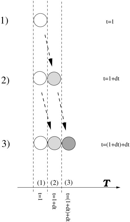
Figure 16: The progress of the universe through increasing times $\sim$ number of elementary cells. As the statistics grows, the configuration gets more complex and differentiated. Configuration 3) does not “include” configuration 2), which in turn does not include number 1): with volume increases also the radius, and the curvature of space decreases. The curvature and therefore the energy levels are different at different times. Configuration 1) “flows” to 2), and 2) to 3) only in the sense that 2) is more similar to 3) than 1) or a configuration with two equal balls are, and therefore this is the most realized “evolutionary path”.

Already at the next step, $N=2$, we have many more (infinitely many) possibilities, corresponding to any possible space “dimension”, being $N^{p}$ no more trivial, and the combinatorics increases very rapidly. For what discussed in section 2.2 we can concentrate the analysis to three dimensions, which gives a contribution of the same amount as the sum of all the neglected dimensionalities and configurations (Uncertainty Principle). The dominant configuration is the one that gives a “homogeneous” distribution of the occupied cells (what at large $N$ becomes a “spheric” geometry) . But already at $N=2$ also non-extremal entropy configurations start to exist and give non-trivial contributions. The result is that, on the top of a homogeneous distributions, in the Universe start to show up inhomogeneities, of the order of the Uncertainty Relations. We can represent this process by distinguishing the regions of the space as balls with a different colour, figure 16. As time goes by (i.e. $N$ increases), we get new possibilities of differentiation from the basic homogeneity, in a sort of “progressive differentiation through steps of small perturbations”. We indicate this with an increasingly darker coloration of the balls. In principle, one could ask if there could be “discontinuities” in this progress, namely, whether there could be steps in which a darker ball falls between lighter balls, as illustrated in figure 17.

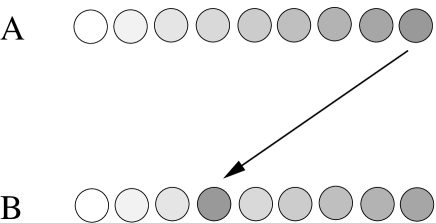
Figure 17: Configuration B) is obtained by superposing to the dominant configuration less entropic configurations than in A), and therefore has a lower weight, the more and more negligible the higher is the “jump” between B) and A).

Of course, nothing prevents such configurations from appearing, and indeed they are present. However, dominance of the most entropic configurations, with deviations milder and milder as the asset departs from the most entropic configuration, tells us that these discontinuities give a minor contribution, so that, in the average, the evolution takes place in the continuous way we illustrate in figure 19.

The progress through times/values of the average curvature and its inhomogeneities looks therefore like the propagation of a perturbation, and is translated, in the continuous language of string theory, into a “propagation” of the information through an expanding universe. As time goes by, the average curvature of space decreases, and this takes place everywhere, throughout all the space. The “perturbations” too spread out: as $1/N^{2}$ for those that we interpret as “massless fields”, or with a lower rate for the “massive” ones. To an observer, the local physics appears to be influenced, “produced” if one prefers, by the sum of the information that propagated up to him from everywhere else in the space. We already mentioned that a detector is a particular configuration of space, and an experiment is the detection of variations of this configuration during a certain interval of time. By letting an experiment, or a detection, to take place in a certain interval of time, the observer can resolve for different “smearing rates” of the inhomogeneities, and consequently organise the interpretation of what happens in terms of massless and/or massive objects. Of course, this is only an approximation, because any possible configuration contributes, however to an uncertainty expressed by the Uncertainty Principle . The “experimental observation” of the universe surrounding an observer indeed carries the information about the geometry of the full universe, the progress toward an increasing “local” differentiation from the average geometry being interpretable as a continuous, “jump-less” evolution that propagates the perturbation of the spheric geometry. String theory provides us with a theoretical framework enabling us to organise the interpretation of this information in terms of particles, fields, interactions etc… What we observe is indeed always just our local physics, but we disentangle the jungle of data by organising them as a superposition of informations coming from different places, and therefore “originating” at different times in the past.

Notice that, although we see regions of the Universe corresponding to past times, we don’t see ourselves in our past times: neighbouring shells are not derived the one from the other through time evolution.

The universe at (any) present time ${\cal T}$ is given by the (weighted) superposition of the configurations of the phase space at present time.

In this sense, the actual configuration depends only on the present phase space, not on the past: the evolution belongs to our interpretation.

For the observer the universe turns out to mainly consist of a progression from the farthest configuration, the “initial” one, to the nearest, representing the physics at present time. At any time, the dominant configuration is however not derived by a process of evolution of the one at previous time, but through a process of entropy maximization at present time.

Figure 18: During the time evolution, the three-dimensional space build up of an increasing number of elementary cells expands with the geometry of a three-sphere of growing radius.

To an observer the space appears built as an “onion”: the observer is surrounded by shells, two-spheres corresponding to farther and older phases of the universe, up to the horizon, that correspond to the “big bang”, as illustrated in figure 19.

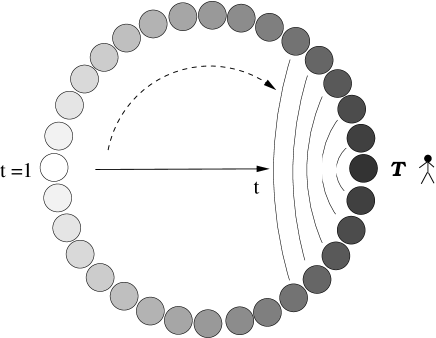
Figure 19: The Universe at time ${\cal T}$ appears to the observer as a set of surrounding shells made out of elementary cells. These shells, here represented only through sections constituted by two linked antipodal cells, go from the one closest to the observer (the darkest one), which is also the closets in time, up to the farthest, the horizon, that corresponds to the “big-bang” cell. The curvature of space is on the other hand everywhere the one of the age corresponding to the observer, ${\cal R}\sim 1/{\cal T}^{2}$. Notice that the two-sphere corresponding to the horizon appears to “conserve” the total energy flux, $1$, of the initial unit cell.

However, in itself there is no real “big-bang point”, located somewhere in this space: the argument leading to this description of the observed Universe is not related to a particular choice of the point of observation. This does not mean that the Universe looks absolutely identical for any choice of this point inside the whole space; simply, it means that from any point the Universe appears built as an “onion”, with informations coming from everywhere around, going backwards in time, and space, up to the horizon, which is an “apparent horizon”, with no real physical location, but always at distance $N\sim{\cal T}$ from the observer.

Wherever the location of the observer in the space is, what he will see is only the “tangent” space around him, experienced through the modifications it produces in himself. In this way, he will have access to the knowledge of the average energy density of the universe, and indeed an indirect experience of the whole universe: the “local physics” is the one specific of the actual time, and as such “knows” about the full extension of the space. Owing to the special “boundary conditions” that “sew” the borders of space into a sphere, the latter will look in the average homogeneous all around in every direction: the observer will always have the impression of being located “at the center” of the Universe. Through the modification of his configuration, the “local physics”, (i.e. the set of all what happens to him, light rays hitting from the various directions, gravitational fields etc…, that he will interpret as coming from all over the space around), he will then “measure” the energy density through all the space, concluding that it is $\rho(E)\sim 1/R^{2}$. On the other hand, knowing that such an energy-density scaling law is the one of a sphere, he will deduce that the horizon surface at a distance $R$ from himself, and with area $\sim R^{2}$, has boundary conditions such that the space closes-up to a sphere. The observer will then interpret the set of cells spread out along the horizon, a surface with area $\sim R^{2}$ and energy density $\sim 1/R^{2}$, as corresponding to a point, a unique cell of unit volume and unit energy, “smeared” over something that appears like a two-sphere. He will therefore refer to this as to the “big-bang” point, the initial configuration, energy one at volume one, and he will say that what he sees by looking at the horizon, is indeed the beginning of everything. We repeat however that this point, or surface, namely, the horizon, does not really exist as a special point located somewhere in space: the interpretation would be the same for any observer, located at whatever point in this space.

7.5 Non-locality and quantum paradoxes

The uncertainty encoded in Quantum Mechanics through the Uncertainty Principle, lifting up the predictive power of classical mechanics to a probabilistic one, leads also to non-locality, possibly violating the bound on the speed of the transfer of information set by the speed of light $c$.

It has been a long debated question, whether this had to be considered as something really built-in in natural phenomena, or simply an effect due to our ignorance of all the degrees of freedom involved, something that could be explained through the introduction of “hidden variables” [5]. It seems that indeed the physical world lies on the side of true quantum interpretation, which, as shown by Bell [6], is not reproducible with hidden variables.

At the quantum level, the bound on the travel speed of information, $c$, can be violated by non-locality of wave-functions. How can we understand all that in the light of our framework?

In our framework, the uncertainty of the Uncertainty Principle, at the base of quantum mechanics, is due to the fact that what we observe and measure is the sum of an infinite number of configurations, among which also tachyonic ones contribute. This is in agreement with the fact that non-locality implies somehow a propagation at speed higher than $c$, thereby violating causality. And indeed, the “dynamics” described in the previous section, resulting from the fact that at any time the universe is the sum of all configurations at the actual time, averaged to the one of maximal entropy, implies in some sense an istantaneous transfer of information, although the classical geometric deformations propagate at maximal speed $c$. Related to this are also other properties, that in our scenario we see as quantum effects on the large, cosmic scale. For instance, the masses themselves. In our framework, masses depend on the space-time size of the universe. This means that, at any time, an electron, or any other particle, “knows” how large is the universe up to the horizon. How would such a boundary information determine the properties of each particle, even those locally produced in laboratory, if any information could only be transferred at maximal speed $c$? This non-local, basically instantaneous knowledge implied in the combinatoric scenario is reproduced in string theory, a relativistic theory, essentially in two ways:

1) through an explicit quantization, in order to reproduce the ordinary quantum effects, which include non-local, tachyonic-like effects such as experiment correlations violating Bell’s inequalities and so on, and

2) through the very basic properties of the string construction, in which, as we discussed in Ref. [1], massive particles live partly in the extended space, identified with the ordinary space-time, the space along w hich they propagate, and partly have a foot in the internal string space.

Roughly speaking, beeing extended also in the internal space provides massive states an extra dimension from which they can “look” at the entire space-time, anyway a compact space, of which they can “see” the boundary, because the internal coordinate is non-local with respect to the external ones (see figure 20).

Figure 20: A pictorial illustration of how can massive particle/fields have knowledge of the full space-time. Here the extended but compact space-time is represented as a disc on the horizontal plane. The internal dimension is represented by the vertical segment. A field/particle confined to live tangent to the space-time cannot “see” the horizon, but just the neighbours of the point where it is sitting. A particle/field with a foot on the internal space can lift-up its point of view and see the horizon, having from above a global view of the disc on the plane.

This is not true for the massless fields (photon and graviton), that live entirely in the extended space-time. They therefore feel only the local physics.

7.5.1 Holography and orbifold

As discussed in [1], the average dominant metric of the Universe, i.e. a three-dimensional sphere, solves the FRW equations for the cosmological evolution of the metric. We have on the other hand seen that the entropy of this universe scales like the entropy of a black hole, namely with the volume of a two-sphere with the same radius. This surface appears as the boundary of the space, that in turn appears to the observer as a ball. Although a three-sphere doesn’t have a boundary, we have nevertheless the impression that the Universe does have a boundary, constituted by the horizon of observation. This “holographic” behaviour may seem contradictory. However, a sphere can be viewed as cut in two “hyperdiscs” by a hypersphere (for instance, a two-sphere is cut by a circle in two discs). If we pair two neighbouring hyperspheres, one serving as boundary for one of these two hyperdiscs, the other to the other one, and we identify these two boundaries, together with the two bulks we build up a sphere. A sphere can therefore be viewed as the union of two hyperdiscs, with a $Z_{2}$ identification of the boundaries (see figure 21).

Figure 21: Space-time is a three-sphere, here represented in lower dimension by a two-sphere. Although without boundary, it can be thought as the union of two hemispheres with neighbouring circles (two-spheres in four space-time dimensions) as boundaries. The two boundaries of the hemispheres are identified by a $Z_{2}$ reflection symmetry.

As such an orbifold, our Universe does have a boundary constituted by a two-sphere. This pair of two-spheres holographically contains the information about the “bulk” (the union of the two “bulks”), which can be thought as the interior of a black hole with, as horizon, one of the two two-spheres. In this way we obtain two times more entropy than what we would expect, corresponding to a rescaling $R\to R/\sqrt{2}$. However, things are re-established to their correct normalization by the $Z_{2}$ orbifold operation.

It is interesting to have a look at the action of this operation on the geometry of this space. As we discussed in Ref. [1], a $Z_{2}$ operation on the extended space coordinates of the string target space is required in order to reach the string configuration of minimal entropy. According to Ref. [1], in the string representation the operation is a pair of freely acting projections, whose effect on the string vacuum is to break parity and time-reversal symmetries, as well as to reduce to a minimum the gauge group, by breaking the weak symmetry group, giving mass to bosons and matter states. The shift on the string side is precisely what is needed in order to 1) reduce the number of massless fields to coincide with the number of space-time dimensions (see discussion in section 7.2). If there are more massless fields, as a matter of fact space is more than three-dimensional. However entropy, which is basically the Jacobian of the transformation from the string frame to the space-time frame (see [1], chapter 4), remains proportional to ${\cal T}^{2}$. This means that we don’t have anymore an $n$-sphere. These configurations are non-extremal and therefore suppressed. 2) The further important effect of the shift is to break parity and time reversal, with the consequence of making possible the identification of the time coordinate of the string target space with the time as we have defined it in this work. Once again, on the string side this is related to a mass shift.

On the side of the geometry of combinatorics, the $Z_{2}$ is an operation that simply identifies two boundaries, something that looks completely unrelated to what happens on the string side. The relation is that on the string side only by lifting massless degrees of freedom we reduce to true three dimensions; only in three dimensions a two-sphere has co-dimension one and can be a boundary for a semi-sphere, in the sense above explained. Otherwise, in higher dimensions we can “pass around” this region, which is not anymore a boundary: from a physical point of view, in this case we can “go beyond the horizon and come back” without problems. We cross therefore the border to tachyonic configurations, and talking of time evolution becomes meaningless. Therefore, the operation on the string side and on the combinatoric side effectively do correspond.

Notice that all these shifts give rise to masses which introduce modifications of the geometry of the order of the Heinsenbergs’s uncertainty relation. This agrees with the fact that non-extremal configurations (among which also tachyonic ones) contribute by an amount of the order of the Heisenberg’s uncertainty (see section 3).

On the string side, the orbifold operation halves the volume of the coordinates it acts on. In order to see that it reduces the radius by a factor $\sqrt{2}$, one can consider that, being space-time a surface spanned by light rays, any operation acting on the time coordinate must also act on a space coordinate. The volume elements are of the type $v=(ds)^{2}=dtdx$. The factor 2 is therefore effectively “distributed” over two coordinates.

7.5.2 Speed of light versus speed of expansion

As we said, to an observer the Universe appears in the average as a “(hyper)disk” bounded by a (hyper)circle, both of them with radius $R=c{\cal T}$, where ${\cal T}$ is the age of the Universe. However, the geometry of space-time is curved, and corresponds to the one of a three-sphere, this too of radius $R=c{\cal T}$. Light paths correspond therefore to geodesics in this curved space. A light beam that appears to the observer to be long as much as $R=c$ times the age of the Universe ${\cal T}$, i.e. coming from the origin of time, corresponding to the horizon as illustrate in picture A of figure 22, in reality follows a curved path, as illustrated on the right in picture B, a path long ${\pi\over 2}c{\cal T}$. The “true” speed of light is therefore higher than the speed of expansion, or equivalently the “scale factor” $R$ of the universe is shorter, and expands at a lower speed, than real distances.

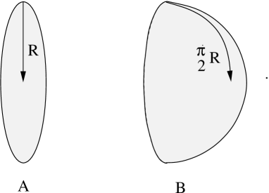
Figure 22: A light ray seen by the observer as coming from the horizon, represented as the boundary of a flat space, the disc of picture A, follows in reality a curved path, a geodesic on the hemisphere depicted in B. The real distance is longer: $R$ in (A) and ${\pi\over 2}R$ in (B).

However, this is of no physical relevance: it does in fact make no sense to ask what is the “real” speed of expansion, the “real” age of the Universe, in a world in which everything looks like if we were living in a flat space bounded by a horizon at distance $R=c{\cal T}$. The only signal of the existence of a curvature comes from indirect experiments, in which cosmological data are interpreted within a theoretical framework. Namely, for what matters parameters such as the energy density of the Universe, the matter content, the speed of expansion of the horizon, and consequently the age of the Universe, everything works consistently with the identification of the speed of light with the speed of expansion, the total energy with the integral of the energy density over the (hyper)disk, i.e. the ball enclosed by the horizon, and the Universe itself with a black hole. For what matters the cosmological evolution too, densities and equations of motion are normalized for a space with boundary, the “ball” enclosed by the horizon. The two scales, either of times or of lengths, are proportional, and any computation of red-shifts and similar parameters is insensitive to this detail.

8 In few words

Let’s summarize in simple words the philosophy of what we are stating in this work. The Universe appears to possess certain properties and has a certain aspect, because this is the most frequently realized configuration. In order to illustrate this point with an example, let’s consider the elementary case of a “universe” consisting just of a plate which, as possible configurations, can either stay at rest, or rotate along the $z$-axis, clockwise or counterclockwise (if this is an electron, or a proton, this schematically reproduces the configurations of spin $0$, spin $+1/2$, spin $-1/2$). The situation is illustrated in figure 23.

Figure 23: A simple system consisting of a plate that can only either stay at rest, or rotate along the two senses of the $z$ axis.

Clearly, we have 1/3 of the probability to see the plate/particle at rest, 1/3 to see it rotating leftwards, 1/3 rotating rightwards. All in all, 2/3 of the times we look at the plate, we see it in rotation, either leftwards or rightwards. In practice, in the average we see a rotating plate, because the situation of “being in rotation” has more possibilities to be realized (rotation clockwise or rotation counterclockwise) than the configuration “plate at rest”. What we “experimentally” conclude is that the plate, with a certain degree of approximation (very rough in this case indeed = 2/3), has a non-vanishing angular momentum. Beyond the 2/3 degree of precision, the spin cannot be measured, because beyond this threshold there is indeed no spin. This example is extremely schematic and by no means reproduces whatever real situation. However, here we see the basic reason why, according to our discussion, the Universe appears to be as it is: protons and electrons have spin because this is the most frequently realized configuration in the phase space, etc… The fully varied spectrum of particles, fields, interactions, galaxy clusters etc… is the effect of being this the configuration of minimal entropy, or equivalently the most frequently realized configuration.

A question arises now: is it life too part of this game? Can we see the existence of life, and the increasing complexity of its forms, as due to the same rationale? Does life exist because, in the appropriate conditions, the chemical processes that we interpret as “life” correspond to the most frequently realized configuration? In principle, nothing seems to forbid it, and indeed at least certain aspects seem to nicely fit within this picture (see Ref. [7]). The hardest point to be accepted is however the fact that, if the entire story of life can be reduced to these same principles, then also human thoughts, actions and decisions, are “determined” (not deterministic though!), although predictable only by knowing an infinite number of degrees of freedom. That means, in practice impossible to predict.

References

- [1] A. Gregori, An entropy-weighted sum over non-perturbative vacua, arXiv:0705.1130 [hep-th].
- [2] M. Rabinowitz, n-dimensional gravity: Little black holes, dark matter, and ball lightning, Int. J. Theor. Phys. 40 (2001) 875–901, astro-ph/0104026.
- [3] A. Gregori, Entropy, string theory, and our world, hep-th/0207195.
- [4] A. Gregori, Naturally time dependent cosmological constant in string theory, hep-th/0402126.
- [5] A. Einstein, B. Podolsky, and N. Rosen, Can Quantum Mechanical Description of Physical Reality Be Considered Complete?, Phys. Rev. 47 (May 15, 1935).
- [6] J. S. Bell, On the Einstein Podolsky Rosen Paradox, Physics 1 (1964) 195–200.
- [7] A. Gregori, A note on the phases of natural evolution, arXiv:0712.0074 [physics.gen-ph].