The variational particle-mesh method for matching curves

Abstract

Diffeomorphic matching (only one of several names for this technique) is a technique for non-rigid registration of curves and surfaces in which the curve or surface is embedded in the flow of a time-series of vector fields. One seeks the flow between two topologically-equivalent curves or surfaces which minimises some metric defined on the vector fields, i.e. the flow closest to the identity in some sense.

In this paper, we describe a new particle-mesh discretisation for the evolution of the geodesic flow and the embedded shape. Particle-mesh algorithms are very natural for this problem because Lagrangian particles (particles moving with the flow) can represent the movement of the shape whereas the vector field is Eulerian and hence best represented on a static mesh. We explain the derivation of the method, and prove conservation properties: the discrete method has a set of conserved momenta corresponding to the particle-relabelling symmetry which converge to conserved quantities in the continuous problem. We also introduce a new discretisation for the geometric current matching condition of (Vaillant and Glaunes, 2005). We illustrate the method and the derived properties with numerical examples.

Keywords: symplectic integrators, diffeomorphic shape matching, geodesics on the diffeomorphism group, EPDiff

For Darryl Holm on the occasion of his 60th birthday

1 Introduction

Diffeomorphic matching is a numerical framework for quantifying the differences between geometric information (such as curves, surfaces, images or vector fields) using deformations from one geometric object to another. The geometric object is embedded in the flow generated by a time-series of vector fields with a chosen norm (such as the $H^{1}$-norm) defining the distance along the path between geometric objects. The computational task is to calculate the velocity fields which minimise this distance such that one geometric object is mapped to another. This framework was originally introduced in a series of papers including [GM98, CY01, MY01, MTY03] being extended to match distributions (which can model curves and surfaces) in [GTY04], and to match geometric currents (also for modelling curves and surfaces) in [VG05]. Various numerical approaches have been proposed for solving the optimisation problem, either by optimising the functional directly (with an extra term to penalise flows which do not map close to the target shape) as described in [BMTY05], or by solving the equations of motion and shooting for a match between shapes by adjusting the initial conditions as in [TMT02, MM06a, MMS06]. The main challenge remains to find a numerical approach which is accurate and efficient, since the problem of computing the shortest path is a high-dimensional optimisation problem.

In this paper we introduce a new numerical discretisation for the diffeomorphic matching problem in the context of matching (although it can also be used for matching surfaces, images and vector fields). This method uses a similar approach to the Hamiltonian Particle-Mesh (HPM) method [FGR02], with the difference being that HPM uses the particle-mesh discretisation to interpolate density from the particles to the mesh, whereas in this application the particle-mesh discretisation is used to interpolate momentum (which takes a central role in the diffeomorphic matching framework).

In section 2 we give a review of the diffeomorphic matching approach applied to curves in the plane, and establish the notation which will be used in the other sections. We also discuss the role of momentum, the conditions used to establish whether the curves have been matched, and the implications of the particle-relabelling symmetry satisfied by the equations of motion, as well as the connection with EPDiff and the Camassa-Holm equation. In section 3 we introduce the particle-mesh discretisation and discuss the discrete symmetries and conservation laws, as well as a discretisation of the current matching condition and a description of solution methods. In section 5 we illustrate the properties of the numerical method applied to computing the shortest path between two test shapes. Finally, in section 6 we give a summary and outlook.

2 Diffeomorphic matching of embedded curves

In this section we describe the problem of matching one embedded curve onto another using diffeomorphisms. For simplicity we shall focus on simple closed curves in the plane although the approach is easily generalised to other structures.

2.1 Parameterisations of curves

We take two simple curves embedded in $\mathbb{R}^{2}$, $C_{A}$ and $C_{B}$, with parameterisations

$$\bi{Q}_{A}(s),\quad\bi{Q}_{B}(s),\qquad s\in[0,2\pi).$$

Note that the curves can equally well be represented by reparameterisations of the curves i.e. by

$$\bi{Q}_{A}(\eta(s)),\quad\bi{Q}_{B}(\eta(s)),\qquad s\in[0,2\pi),$$

where $\eta(s)$ is a diffeomorphism of the circle. Our aim is to find a matching process which is independent of such reparameterisations.

2.2 Curves embedded in a flow

If we take a vector field which defines a fluid flow $\bi{u}(\bi{x},t)$, and embed a curve in that flow, then the curve satisfies

$$\frac{\partial}{\partial t}\bi{Q}(t;s)=\bi{u}(\bi{Q}(t;s),t),$$ (1)

i.e. each point of the curve moves with the vector evaluated at that point.

The aim of the calculation is to search amongst time-series of vector fields $\bi{u}(\bi{x},t)$, $t\in[0,1]$ such that (1) is satisfied, with the boundary conditions

$$\bi{Q}(0;s)=\bi{Q}_{A}(s),\quad\bi{Q}(1;s)=\bi{Q}_{B}(\eta(s)),$$

for some (unspecified) reparameterisation $\eta$. If these conditions are satisfied then we say that $\bi{Q}_{A}$ is matched onto $\bi{Q}_{B}$ by the vector field time series $\bi{u}(\bi{x},t)$.

2.3 Optimisation problem

We choose a norm for vector fields, such as the $H^{n}_{\alpha}$ norm defined by

$$\|\bi{u}\|^{2}_{H^{n}_{\alpha}}=\int_{\mathbb{R}^{2}}\bi{u}(\bi{x})\cdot(1-\alpha^{2}\nabla^{2})^{n}\bi{u}(\bi{x})\rmd\mathrm{Vol}(\bi{x})$$

Given a time series $\bi{u}(\bi{x},t)$, we can measure the total amount of deformation in the flow generated by $\bi{u}$ by the integral

$$S(\bi{u})=\int_{0}^{1}\frac{1}{2}\|\bi{u}\|^{2}\rmd t.$$ (2)

We wish to find the flow that maps $C_{A}$ to $C_{B}$ which is “nearest to the identity” with respect to the choice of norm. This leads to the following optimal control problem [GTY06]:

Definition 1 (Optimisation problem for curve matching)

Let $\bi{Q}_{A},\bi{Q}_{B}:S^{1}\to\mathbb{R}^{2}$ be parameterisations of two curves $C_{A}$, $C_{B}$ in the plane, and let $\|\cdot\|^{2}$ be a norm for vector fields in the plane. Then the distance between curve $C_{A}$ and $C_{B}$ is defined to be the minimum over all vector fields $\bi{u}$ of the functional

$$\int_{0}^{1}\frac{1}{2}\|\bi{u}\|^{2}\rmd t$$

subject to the following constraints:

• Dynamic constraint: $\frac{\partial}{\partial t}\bi{Q}(t;s)=\bi{u}(\bi{Q}(t;s),t)$, $\forall t\in[0,1]$.

• Matching conditions: $\bi{Q}(0;s)=\bi{Q}_{A}(s)$, $\bi{Q}(1;s)=\bi{Q}_{B}(\eta(s))$, where $\eta$ is some reparameterisation of the circle.

2.4 Momentum

We can enforce the dynamic constraint by introducing Lagrange multipliers $\bi{P}(t;s)$, so that the optimisation problem becomes

$$\delta\int_{0}^{1}\frac{1}{2}\|\bi{u}\|^{2}+\int_{s=0}^{2\pi}\bi{P}\cdot(\dot{\bi{Q}}-\bi{u}(\bi{Q}))\rmd s\rmd t=0,$$ (3)

subject to the matching conditions give above. The Euler-Lagrange equations then give

$$\frac{\delta l}{\delta\bi{u}} = \int_{s=0}^{2\pi}\bi{P}\delta(\bi{x}-\bi{Q})\rmd s,$$ (4)

$$\dot{\bi{Q}} = \bi{u}(\bi{Q}),$$ (5)

$$\dot{\bi{P}} = -\bi{P}\cdot\nabla\bi{u}(\bi{Q}),$$ (6)

where $l=\|\bi{u}\|^{2}/2$. For example, if we choose the $H^{n}_{\alpha}$-norm then

$$\frac{\delta l}{\delta\bi{u}}=(1-\alpha^{2}\nabla^{2})^{n}\bi{u}.$$

We see that optimal velocity fields take the form

$$\int_{s=0}^{2\pi}\bi{P}G(\bi{x}-\bi{Q})\rmd s,$$ (7)

where $G$ is the Green’s function associated with the chosen norm, e.g. for the $H^{n}_{\alpha}$-norm it is the Green’s function for the operator $(1-\alpha^{2}\nabla^{2})^{n}$.

Equation (4) allows us to write $\bi{u}$ as a function of $\bi{P}$ and $\bi{Q}$, leading us to notice that equations (5-6) are canonically Hamiltonian, with Hamiltonian function given by

$$H=l(\bi{u}(\bi{P},\bi{Q}))=\frac{1}{2}\|\bi{u}(\bi{P},\bi{Q})\|^{2},$$

i.e., half the square of the norm of the velocity field written as a function of $\bi{P}$ and $\bi{Q}$. It is for this reason that we refer to the Lagrange multiplier $\bi{P}$ as the momentum associated with the curve. This Hamiltonian structure arises from the fact that the equations have been derived from a variational principle defined by the extreme points of the functional. Since the Hamiltonian for this system is time-independent, it is conserved along the trajectory, and hence the norm of the velocity is also conserved.

2.5 Matching condition

There are a number of different possible ways to pose the matching condition mathematically. One matching condition which is invariant under reparameterisations is based on defining a singular vector field

$$\bi{v}^{\bi{Q}}(\bi{x})=\int_{s=0}^{2\pi}\frac{\partial\bi{Q}}{\partial s}\delta(\bi{x}-\bi{Q})\rmd s.$$ (8)

We define a functional for these singular vector fields

$$f\left[\bi{v}^{\bi{Q}}\right] = \int\bi{v}^{\bi{Q}}\cdot K*\bi{v}^{\bi{Q}}\rmd\mathrm{Vol}(\bi{x})$$ (9)

$$= \int_{s=0}^{2\pi}\frac{\partial\bi{Q}}{\partial s}\cdot\int_{s^{\prime}=0}^{2\pi}\frac{\partial\bi{Q}}{\partial s^{\prime}}K(\bi{Q}(s)-\bi{Q}(s^{\prime}))\rmd s\rmd s^{\prime}.$$

where $K$ is some smooth kernel function. When $\bi{Q}$ matches $\bi{Q}_{B}$ then $f[\bi{v}^{\bi{Q}}-\bi{v}^{\bi{Q}_{B}}]$ vanishes. This is called the current matching condition [VG05].

This is a weaker condition that setting the value of $\bi{Q}(s)$ for each $s$ at time $t=1$, and hence we need to add another boundary condition to get a unique solution to equations (4-6). In [MTY03] it was shown that the solution which minimises the functional is the one with $\bi{P}$ initially normal to the curve i.e.

$$\bi{P}\cdot\frac{\partial\bi{Q}}{\partial s}=0,\qquad\mathrm{at}\quad t=0,$$

and this extra boundary condition means that equations (4-6) have a unique solution.

2.6 Relabelling

The optimisation problem in definition 1 is invariant under symmetries given by reparameterisations of the curve $\eta$. Noether’s theorem tells us that the equations of motion (4-6) have conserved quantities which are generated by these symmetries.

To compute the conserved quantities we compute the infinitesimal generators of these symmetries

$$\delta\bi{Q}(s;t)=\frac{\partial\bi{Q}}{\partial s}\cdot\xi(s)$$

where $\xi(s)$ is a vector field on the circle. The cotangent lift of this infinitesimal symmetry is

$$\delta\left(\bi{Q}(s;t),\bi{P}(s;t)\right)=\left(\frac{\partial\bi{Q}}{\partial s}\cdot\xi(s),-\bi{P}(s;t)\cdot\frac{\partial\bi{Q}}{\partial s}\cdot\xi(s)\right)$$

which is a Hamiltonian flow generated by the Hamiltonian functional

$$h_{\xi}=\int_{s=0}^{2\pi}\bi{P}(s)\cdot\frac{\partial\bi{Q}}{\partial s}\cdot\xi(s)\rmd s.$$

By Noether’s theorem, $h_{\xi}$ is conserved along solutions of (4)-(6), and since $\xi(s)$ is arbitrary, we see that

$$\bi{P}(s)\cdot\frac{\partial\bi{Q}}{\partial s}$$

is conserved along solution trajectories, for each $s$. In particular, this means that if the momentum is initially normal to the curve i.e.

$$\bi{P}(s;0)\cdot\frac{\partial\bi{Q}}{\partial s}(s;0)=0,$$

then the momentum is normal to the curve for all values of $t$ along the solution. Therefore, optimal velocity fields take the form of equation (7) with the added constraint that the momentum $\bi{P}$ is normal to the curve.

2.7 EPDiff

As described in [CH, CHH07], because the dynamic constraint is given by a Lie algebra action of velocity fields on embedded curves, it is possible to eliminate $\bi{P}$ and $\bi{Q}$ by taking the time derivative of equation (4) and making use of equations (5-6). This leads to a PDE defined on the whole of $\mathbb{R}^{2}$ given by

$$\bi{m}_{t}+\nabla\cdot(\bi{u}\bi{m})+(\nabla\bi{u})^{T}\bi{m}=0,\qquad\bi{m}=\frac{\delta l}{\delta\bi{u}}.$$

This is the Euler-Poincáre equation on the diffeomorphism group, abbreviated as EPDiff [HM04, HMR98], which is the equation for geodesic flow on the diffeomorphism group. Although we do not explicitly solve EPDiff during the computation of the optimal flow, it is useful to understand the computed solutions as singular solutions of EPDiff. In one dimension and with the $H^{1}_{\alpha}$-norm, EPDiff becomes the Camassa-Holm equation [CH93] which is completely integrable with singular soliton solutions.

3 Particle-mesh discretisation

We take a discrete mechanics and optimal control [JMOB05] approach by applying the discretisation directly to the functional (3) and deriving the resulting equations. The discretisation used is a particle-mesh method with:

• the vector fields discretised on a fixed, finite mesh, and

• the curve discretised as a set of moving points.

The principle benefits of this discretisation are that different norms can be defined on the mesh without the need to calculate Green’s functions. With large numbers of points the method becomes very efficient as particle momenta can be interpolated to the mesh, then the norm operator can be inverted, then the velocity values can be interpolated back to the particle positions.

3.1 Mesh discretisation of vector fields

We take a fixed set of points on a mesh $\{\bi{x}_{k}\}_{k=1}^{n_{g}}$ (for the numerical examples in this paper we used an equispaced square mesh) and give each mesh point $\bi{x}_{k}$ a vector $\bi{u}_{k}$. We interpolate from the set $\{\bi{u}_{k}\}_{k=1}^{n_{g}}$ of vectors to a general point $\bi{x}$ in the plane using a linear interpolation

$$\bi{u}(\bi{x})=\sum_{k=1}^{n_{g}}\bi{u}_{k}\psi_{k}(\bi{x}).$$ (10)

For the examples in this paper we set $\psi_{k}$ to be a tensor product of cubic B-spline functions centred on $\bi{x}=\bi{x}_{k}$.

Remark 2

The set of vectors on the mesh generate a finite dimensional subspace of the infinite dimensional space of vector fields. However, the finite dimensional subspace is not closed under the Lie bracket for vector fields which means we will not be able to obtain a discrete EPDiff equation from the discrete equations of motion by eliminating $\bi{Q}$ and $\bi{P}$ as in section (2.7).

Once we have this discrete representation of the vector fields we can define a discretised norm using standard mesh methods (such as finite difference, finite volume etc.). For the the examples in this paper we took periodic boundary conditions, and used a spectral discretisation of the $(1-\alpha^{2}\nabla^{2})^{n}$ operator using discrete Fourier transforms, and a simple Riemann sum for the integration (which gives spectral accuracy in this case). Since the Green’s functions decay exponentially over the lengthscale $\alpha$, the boundary conditions should not affect the solution as long as the curve is sufficiently far from the boundary. Other boundary conditions are possible if, for example, a finite-difference method is used to discretise the norm operator.

3.2 Particle discretisation of curves

We replace the parameterised curve $\bi{Q}(s)$ by a finite set of points in the plane $\{\bi{Q}_{\beta}\}_{\beta=1}^{n_{p}}$. The equation (1) gets replaced by the semi-discrete (continuous time/discrete space) equation

$$\dot{\bi{Q}}_{\beta}=\sum_{k=1}^{n_{g}}\bi{u}_{k}\psi_{k}(\bi{Q}_{\beta}).$$ (11)

We also have to choose a discretisation of integration around the loop; again for the examples in this paper we use a Riemann sum.

3.3 Semi-discrete functional and equations of motion

After the particle-mesh discretisation we obtain a semi-discrete functional by integrating the discrete vector field norm from $t=0$ to $t=1$ and introducing Lagrange multipliers to enforce the constraint (11) to get

$$\int_{0}^{1}\frac{1}{2}\|\bi{u}\|^{2}_{g}+\sum_{\beta}\bi{P}_{\beta}\cdot\left(\dot{\bi{Q}}_{\beta}-\sum_{k=1}^{n_{g}}\bi{u}_{k}\psi_{k}(\bi{Q}_{\beta})\right)\rmd t.$$ (12)

The Euler-Lagrange equations for the optimal values of this functional are

$$\frac{\partial}{\partial\bi{u_{k}}}\frac{1}{2}\|\bi{u}\|^{2}_{g} = \sum_{\beta}\bi{P}_{\beta}\psi_{k}(\bi{Q}_{\beta}),$$ (13)

$$\dot{\bi{Q}}_{\beta} = \sum_{k=1}^{n_{g}}\bi{u}_{k}\psi_{k}(\bi{Q}_{\beta}),$$ (14)

$$\dot{\bi{P}}_{\beta} = -\bi{P}_{\beta}\cdot\sum_{k}\bi{u}_{k}\nabla\psi_{k}(\bi{Q}_{\beta}).$$ (15)

Once again, equation (13) allows us to write $\bi{u}$ as a function of $\bi{P}$ and $\bi{Q}$, leading us to notice that equations (14-15) are canonically Hamiltonian, with Hamiltonian function given by $\|\bi{u}(\bi{P},\bi{Q})\|^{2}_{g}/2$.

3.4 Time discretisation

Equation (11) can be discretised using any one-step method, such as a Runge-Kutta method. For simplicity, in this paper we use the forward Euler discretisation, but the derivation of the equations is very similar for other methods. The equation becomes

$$\bi{Q}^{n+1}_{\beta}=\bi{Q}^{n}_{\beta}+\Delta t\sum_{k}\bi{u}^{n+1}\psi_{k}(\bi{Q}^{n}).$$

The discrete functional becomes

$$\sum_{n=1}^{N}\left(\Delta t\frac{1}{2}\|\bi{u}\|^{2}_{g}+\sum_{\beta}\bi{P}^{n+1}_{\beta}\cdot\left(\bi{Q}^{n+1}_{\beta}-\bi{Q}^{n}_{\beta}-\Delta t\sum_{k=1}^{n_{g}}\bi{u}_{k}^{n+1}\psi_{k}(\bi{Q}_{\beta}^{n})\right)\right),$$ (16)

where $\Delta t=1/N$, and the discrete Euler-Lagrange equations are

$$\frac{\partial}{\partial\bi{u_{k}}}\frac{1}{2}\|\bi{u}^{n+1}\|^{2}_{g} = \sum_{\beta}\bi{P}_{\beta}^{n+1}\psi_{k}(\bi{Q}_{\beta}^{n}),$$ (17)

$$\bi{Q}^{n+1}_{\beta} = \bi{Q}^{n}_{\beta}+\Delta t\sum_{k}\bi{u}^{n+1}_{k}\psi_{k}(\bi{Q}_{\beta}^{n}),$$ (18)

$$\bi{P}^{n+1}_{\beta} = \bi{P}^{n}_{\beta}-\Delta t\bi{P}^{n+1}\cdot\sum_{k}\bi{u}_{k}^{n+1}\nabla\psi_{k}(\bi{Q}_{\beta}^{n}).$$ (19)

These equations provide a variational integrator [LMOW03] for the semi-discrete equations (13-15). Hence, they give a symplectic integrator (see [LR05] for a survey of these methods) for the semi-discrete equations in Hamiltonian form. In this particular case we obtain the first-order symplectic Euler method; higher-order partitioned Runge-Kutta methods can be obtained by discretising (11) using any Runge-Kutta method.

3.5 Discrete symmetries

In this section we discuss the properties of applying a variational integrator to equations (13)-(15), and their possible benefits for the problem of matching curves.

The properties that make variational integrators the best choice for long integrations are:

• Modified Hamiltonian: if the Hamiltonian $H(\bi{P},\bi{Q})$ is analytic then it is possible to use backward error analysis to find a modified Hamiltonian

  $$\tilde{H}=H+\Delta t^{p}\Delta H(\bi{P},\bi{Q};\Delta t)$$

  which is conserved over times

  $$|t|\leq c_{0}\exp^{c_{1}/\Delta t}.$$

  See [LR05] for a summary and references.

• Conserved momenta: if the continuous-time Euler-Lagrange equations have conserved momenta associated with symmetries of the Lagrangian, then discrete Euler-Lagrange equations also conserve these momenta [LMOW03].

3.6 Modified Hamiltonian

In the problem of matching curves, the Hamiltonian is half the squared norm for vector fields, which is conserved along trajectories as described in section 2.4. If a symplectic integrator is used then backward error analysis guarantees that the Hamiltonian will be approximately conserved for long times (although it should be noted that no theory exists for the piecewise-cubic functions used in the examples of this paper). It remains an open question as to whether the conservation of the Hamiltonian is important for these problems on finite-time intervals, since they are on short time intervals and so the value of the Hamiltonian will also be approximately preserved by variable step-size methods using error control.

The main cost of using variational integrators is that they are implicit for this type of system where the Hamiltonian is a function of $\bi{P}$ and $\bi{Q}$, but during the optimisation algorithm we are able to store values along the trajectory from previous integrations which can be used as initial guesses for solving the implicit equations using Newton iteration. The variational integrator allows large timesteps to be taken in that case (although of course this is the case for any implicit method, symplectic or otherwise).

3.7 Momentum conservation

As described in section 2.6, the equations (4-6) have a symmetry under reparameterisation of the curve which has an associated conserved momentum $\bi{P}\cdot\partial\bi{Q}/\partial s$. This means that for the optimal solution, $\bi{P}$ remains normal to the curve along the trajectory. Since we have discretised the curve we have broken that symmetry, but as we shall show in this section, it is still possible to recover a sense in which $\bi{P}$ is normal to the curve along the solution.

Equation (10) defines a vector field over the whole space parameterised by the vectors $\{\bi{u}_{k}\}_{k=1}^{n_{g}}$ associated with the mesh points. This means that we can choose a parameterised curve $\bi{Q}(s)$ which passes through our discrete points $\{\bi{Q}_{\beta}\}_{\beta=1}^{n_{p}}$ in sequence and follow its evolution along the flow by solving

$$\frac{\partial}{\partial t}\bi{Q}(s)=\sum_{k}\bi{u}_{k}\psi_{k}(\bi{Q}(s)).$$ (20)

More generally, we can follow how the flow generated by the vector fields evolves over the whole space

$$\frac{\partial}{\partial t}\bi{g}(\bi{x},t)=\sum_{k}\bi{u}_{k}\psi_{k}(\bi{g}(\bi{x},t)),$$

where $g(\bi{x},t)$ is the flow map taking points from their position at time $0$ to their position at time $t$ ($\bi{x}$ plays the role of a coordinate on “label space” here), and we can follow the Jacobian of this map

$$\frac{\partial}{\partial t}\frac{\partial\bi{g}(\bi{x},t)}{\partial\bi{x}}=\sum_{k}\bi{u}_{k}\nabla\psi_{k}(\bi{g}(\bi{x},t))\cdot\frac{\partial\bi{g}(\bi{x},t)}{\partial\bi{x}}.$$

In particular, we can evaluate this equation at each of our discrete points $\bi{Q}_{\beta}$:

$$\dot{J}_{\beta}=\sum_{k}\bi{u}_{k}\nabla\psi_{k}(\bi{Q}_{\beta})\cdot J_{\beta},\qquad J_{\beta}=\frac{\partial\bi{g}}{\partial\bi{x}}(\bi{Q}_{\beta}(0),t),\qquad J_{\beta}(0)=\mathrm{Id}.$$ (21)

A variation $\delta\bi{Q}_{\beta}(0)$ in the initial conditions $\bi{Q}_{\beta}(0)$ leads to a variation in the entire trajectory given by

$$\delta\bi{Q}_{\beta}(t)=J_{\beta}(t)\delta\bi{Q}_{\beta}(0).$$ (22)

This variation generates a symmetry of the equations, as shown in the following lemma.

Lemma 3

The infinitesimal transformation given by equations (21)-(22) together with

$$\delta\bi{P}_{\beta}=0,\quad\beta=1,\ldots,n_{p},\qquad\delta\bi{u}_{k}=0,\quad k=1,\ldots,n_{k},$$

is a symmetry of equations (13)-(15).

Proof. Since the equations have been derived from an action principle, we simply need to show that the infinitesimal transformation causes the action (12) to vanish. If we apply the transformation to the integrand (the Lagrangian) then we obtain

$$\delta L = \delta\left(\frac{1}{2}\|\bi{u}\|^{2}_{g}+\sum_{\beta}\bi{P}_{\beta}\cdot\left(\dot{\bi{Q}}_{\beta}-\sum_{k=1}^{n_{g}}\bi{u}_{k}\psi_{k}(\bi{Q}_{\beta})\right)\right),$$

$$= \sum_{\beta}\bi{P}_{\beta}\cdot\left(\delta\dot{\bi{Q}}_{\beta}-\sum_{k=1}^{n_{g}}\bi{u}_{k}\nabla\psi_{k}(\bi{Q}_{\beta})\cdot\delta\bi{Q}_{\beta}\right),$$

$$= \sum_{\beta}\bi{P}_{\beta}\cdot\left(\dot{J}_{\beta}\cdot\delta\bi{Q}_{\beta}(0)-\sum_{k=1}^{n_{g}}\bi{u}_{k}\nabla\psi_{k}(\bi{Q}_{\beta})\cdot J_{\beta}\delta\bi{Q}_{\beta}(0)\right),$$

$$= \sum_{\beta}\bi{P}_{\beta}\cdot\left(\sum_{k}\bi{u}_{k}\nabla\psi_{k}(\bi{Q}_{\beta})\cdot{J}_{\beta}\cdot\delta\bi{Q}_{\beta}(0)-\sum_{k=1}^{n_{g}}\bi{u}_{k}\nabla\psi_{k}(\bi{Q}_{\beta})\cdot J_{\beta}\delta\bi{Q}_{\beta}(0)\right),$$

$$= 0,$$

and hence the result.

$\square$

This symmetry of the equations has an associated conserved momenta following Noether’s theorem, as described in the following proposition.

Proposition 4

For each $\beta=1,\ldots,n_{p}$, the quantity $J^{T}_{\beta}\bi{P}_{\beta}$ is conserved.

Proof. Applying the symmetry to the action principle and substituting the equations of motion (13)-(15) gives

$$0 = \delta\int_{0}^{1}\frac{1}{2}\|\bi{u}\|^{2}_{g}+\sum_{\beta}\bi{P}_{\beta}\cdot\left(\dot{\bi{Q}}_{\beta}-\sum_{k=1}^{n_{g}}\bi{u}_{k}\psi_{k}(\bi{Q}_{\beta})\right)\rmd t$$

$$= \int_{0}^{1}\sum_{\beta}\left(\dot{\bi{Q}}_{\beta}-\sum_{k=1}^{n_{g}}\bi{u}_{k}\psi_{k}(\bi{Q}_{\beta})\right)\cdot\delta\bi{Q}_{\beta}$$

$$\quad+\frac{\rmd}{\rmd t}\left(\sum_{\beta}\bi{P}_{\beta}J_{\beta}\cdot\delta\bi{Q}_{\beta}(0)\right)\rmd t$$

$$= \sum_{\beta}\left(\bi{P}_{\beta}(t_{1})J_{\beta}(t_{1})-\bi{P}_{\beta}(t_{0})J_{\beta}(t_{0})\right)\cdot\delta\bi{Q}_{\beta}(0).$$

We obtain the result since $\delta\bi{Q}_{\beta}(0)$ is an arbitrary vector.

$\square$

As described in [LMOW03], these conservation laws satisfied by the semi-discrete equations will be preserved by numerical methods provided that they are derived from a discrete variational principle i.e. following the framework described in section 3.4.

If we choose a continuous curve through our set of points that moves with the flow according to equation (20), then an approximation to $\partial\bi{Q}(s_{\beta})/\partial s\cdot\rmd s$ is given at time $t$ by

$$J_{\beta}\Delta\bi{Q}_{\beta}(0),\qquad\beta=1,\ldots,n_{p},$$

where $\Delta\bi{Q}_{\beta}(0)$ is an approximation to $\partial\bi{Q}(s_{\beta})/\partial s\cdot\rmd s$ at time $t=0$. This leads to the following corollary:

Corollary 5

If $\bi{P}_{\beta}$ is chosen to be normal to $\Delta\bi{Q}_{\beta}(0)$ at time $t=0$ for all $\beta$ i.e. $\bi{P}$ is initially normal to the curve, then $\bi{P}$ is normal to $J_{\beta}\Delta\bi{Q}_{\beta}(0)$ for all $t$ along the flow, i.e. $\bi{P}$ stays normal to the curve.

Proof. For each $\beta=1,\ldots,n_{p}$, the component of $\bi{P}$ tangential to the shape is

$$\bi{P}_{\beta}(t)\cdot J_{\beta}(t)\Delta\bi{Q}_{\beta}(0) = \bi{P}_{\beta}(0)\cdot J_{\beta}(0)\Delta\bi{Q}_{\beta}(0)$$

$$= \bi{P}_{\beta}(0)\cdot\mathrm{Id}\Delta\bi{Q}_{\beta}(0)$$

$$= \bi{P}_{\beta}(0)\Delta\bi{Q}_{\beta}(0)=0.$$

$\square$

If the equations of motion for $\bi{Q}$ and $\bi{P}$ are discretised using a variational integrator then this property is preserved, provided that the discrete equation for the evolution of $J$ is defined as the gradient of the evolution equation for $\bi{Q}$, since then it generates a symmetry of the discrete variational principle just as in the continuous time case.

For example, the discrete equation for the gradient of the time-discrete flow for $\bi{Q}$ obtained from the symplectic Euler method is

$$J_{\beta}^{n+1}=J_{\beta}^{n}+\Delta t\sum_{k}\bi{u}_{k}^{n+1}\nabla\psi(\bi{Q}_{\beta}^{n})J_{\beta}^{n}.$$ (23)

Proposition 6

For each $\beta=1,\ldots,n_{p}$, the quantity $J^{T}_{\beta}\bi{P}_{\beta}$ is conserved when the equations are integrated using the symplectic Euler method, and $J$ is obtained from equation 23.

Proof.

$$\delta A = \delta\sum_{n=1}^{N}\left(\frac{1}{2}\Delta t\|\bi{u}\|^{2}_{g}+\sum_{\beta}\bi{P}^{n+1}_{\beta}\cdot\left(\bi{Q}^{n+1}_{\beta}-\bi{Q}^{n}_{\beta}-\Delta t\sum_{k=1}^{n_{g}}\bi{u}_{k}^{n+1}\psi_{k}(\bi{Q}_{\beta}^{n})\right)\right),$$

$$= \sum_{n=1}^{N}\left(\sum_{\beta}\bi{P}^{n+1}_{\beta}\cdot\left(\delta\bi{Q}^{n+1}_{\beta}-\delta\bi{Q}^{n}_{\beta}-\sum_{k=1}^{n_{g}}\bi{u}_{k}^{n+1}\nabla\psi_{k}(\bi{Q}_{\beta}^{n})\cdot\delta\bi{Q}_{\beta}^{n}\right)\right),$$

$$= \sum_{n=1}^{N}\sum_{\beta}\bi{P}^{n+1}_{\beta}\cdot\left((J_{\beta}^{n+1}-J_{\beta}^{n})\cdot\delta\bi{Q}_{\beta}^{0}-\sum_{k=1}^{n_{g}}\bi{u}_{k}^{n+1}\nabla\psi_{k}(\bi{Q}_{\beta}^{n})\cdot J_{\beta}^{n}\delta\bi{Q}_{\beta}^{0}\right),$$

$$= \sum_{\beta}\bi{P}_{\beta}^{n+1}\cdot\left(\sum_{k}\bi{u}_{k}^{n+1}\nabla\psi_{k}(\bi{Q}_{\beta}^{n})\cdot{J}_{\beta}^{n}\cdot\delta\bi{Q}_{\beta}^{0}-\sum_{k=1}^{n_{g}}\bi{u}_{k}^{n+1}\nabla\psi_{k}(\bi{Q}_{\beta}^{n})\cdot J_{\beta}^{n}\delta\bi{Q}_{\beta}^{0}\right),$$

$$= 0,$$

Applying the symmetry to the discrete action principle 16 and substituting the equations of motion (13)-(15) gives

$$0 = \sum_{\beta}\left(\bi{P}_{\beta}^{n+1}J_{\beta}^{n+1}-\bi{P}_{\beta}^{n}J_{\beta}^{n}\right)\cdot\delta\bi{Q}_{\beta}^{0}.$$

We obtain the result since $\delta\bi{Q}_{\beta}^{0}$ is an arbitrary vector. $\square$

We can verify the discrete conservation of $\bi{P}_{\beta}J_{\beta}$ directly since

$$\bi{P}^{n}_{\beta}J_{\beta}^{n} = \bi{P}^{n+1}_{\beta}(\mathrm{Id}+\sum_{k}\bi{u}_{k}^{n+1}\nabla\psi_{k}(\bi{Q}^{n}_{\beta}))J_{\beta}^{n}$$

$$= \bi{P}^{n+1}_{\beta}J^{n+1}_{\beta}.$$

Similar results can be obtained when higher-order variational integrators are used by discretising the $\bi{Q}$ equation using a Runge-Kutta method.

As discussed in section 2.5, the norm-minimising solution has momentum normal to the shape along the whole trajectory. Good preservation of the tangential component of momentum is important because it means that it is only necessary to constrain the momentum to be normal to the shape in the initial conditions when a shooting algorithm is used (discussed in section 4).

3.8 Discrete matching condition

We can also apply a particle-mesh discretisation to the matching condition described in section 2.5. The particle-mesh representation of equation (8) is

$$\bi{v}^{\bi{Q}}_{k}=\sum_{\beta}\Delta\bi{Q}_{\beta}\psi_{k}(\bi{Q}_{\beta}),$$

where $\Delta\bi{Q}_{\beta}$ is an approximation to $\partial\bi{Q}(s)/\partial s\,\rmd s$ at $s=s_{\beta}$. For example, a simple finite difference approximation gives

$$\bi{v}^{\bi{Q}}_{k}=\sum_{\beta}(\bi{Q}_{\beta}-\bi{Q}_{\beta-1})\psi_{k}(\bi{Q}_{\beta}).$$

This is the approximation which we will use in the computed numerical examples used in this paper.

Once the singular vector field is evaluated on the mesh we can apply standard mesh discretisation methods to compute the functional (9):

$$\hat{f}[\bi{v}^{\bi{Q}}]=\sum_{kl}K_{kl}\bi{v}^{\bi{Q}}_{k}\bi{v}^{\bi{Q}}_{l}$$

where $K_{kl}$ is a discretisation of the kernel operator $K$. For the computed numerical examples used in this paper, the kernel operator used was the inverse operator $(1-\alpha^{2}\nabla^{2})^{-2}$ discretised using discrete Fourier transforms.

This results in a numerical discretisation of the functional used for the current matching condition. After numerical discretisation the functional will not have a minimum at zero any more, and we must aim to minimise this functional rather than find the zero to achieve matching.

3.9 Efficiency

In [VG05], a mesh-free method was applied to the current matching problem. The main cost in this type of method is in summing up Green’s functions on each of the points on the curve to calculate their velocity, and the value of the matching condition. They employed a fast multipoles algorithm [GS91] which has a computational cost of size $\mathcal{O}(N\log N)$ (where $N$ is the total number of particles), although the multiplicative constant in the scaling can be relatively big, requiring larger $N$ before benefits are seen.

For a particle-mesh method, the cost of evaluating the momentum on the grid is $\mathcal{O}(N)$, and the cost of the FFT is $\mathcal{O}(M^{2}\log M)$ (where $M$ is the number of rows of gridpoints i.e. the total number of grid points is $M^{2}$), although one could reduce this by discretising the operator used in the norm for velocity (e.g. the Helmholtz operator in the examples given here) and just performing a few iterations of a method such as Jacobi, resulting in an $\mathcal{O}(M^{2})$ cost. In the case where one is matching dense information (images or measures, for example), then typically $N=cM^{2}$ (with $c>1$) and the particle-mesh approach produces a method which is competitive with fast multipoles methods. For the case of matching curves, typically $N=cM$ (with $c>1$) and a good fast multipole implementation will be more efficient. However, any mesh-based operator inversion is easily parallelised using standard methods (as is the particle-mesh operation), and so this could be a strength of the particle-mesh approach in the curve case. There are also other advantages to using a mesh, for example it is very easy to modify the operator to investigate the behaviour with different kernels.

4 Solution methods

As discussed in section 3.8, numerical discretisation of the matching condition means that we cannot require that the matching functional vanishes, and so we must take this into account in the solution approach. There are two main approaches to obtaining a numerical approximation to the optimal flow between embedded curves:

1. Inexact matching: In this approach, suggested in [MTY03], we “softly” enforce the matching condition by adding a penalty term to the functional (2):

   $$S(\bi{u})=\int_{0}^{1}\|\bi{u}\|^{2}\rmd t+\frac{1}{\sigma^{2}}f[\bi{v}^{\bi{Q}}].$$ (24)

   One then attempts to minimise this functional directly by applying a descent algorithm (such as nonlinear conjugate gradients) by varying the time series of vector fields and computing the implicit gradient of the functional $f$. An alternative method is to introduce the dynamical constraint using the Lagrange multipliers $\bi{P}$ as in section 2.4, and to solve the resulting Euler-Lagrange equations (4-6) (modified to accomodate the penalty functional) using Newton iteration. This approach becomes attractive when it is possible to find a good initial guess at the solution e.g. by specifying a path of curves between $C_{A}$ and $C_{B}$ and approximately solving equation (6) to get an initial guess for $\bi{P}$ given the initial guess for $\bi{Q}$.

   It is worth mentioning that the minimisation of the functional 24 becomes ill-conditioned as $\sigma\to 0$ and so it is not always possible to match one curve onto another with the desired accuracy (or to within the size of numerical errors, having discretised the functional). A modification of the functional called method of multipliers, described in [Ber82], introduces Lagrange multiplier variables along with the penalty parameter $\sigma$ and allows a reduction of the error in matching without making $\sigma$ arbitrarily large.

2. Minimisation by shooting: In this approach, advocated in [MM06b], we seek initial conditions for $\bi{P}$ such that the functional 9 is minimised. The gradient of the functional with respect to the initial conditions for $\bi{P}$ is computed by solving the Euler-Lagrange equations (4-6) from $t=0$ to $t=1$ with those initial conditions, computing the gradients of $f[\bi{u}^{\bi{Q}^{N}}]$ with respect to $\bi{Q}^{N}_{\beta}$, and propagating those gradients back to $\bi{P}^{0}_{\beta}$ using the adjoint equations (see [Gun03], for example). The problem can then be solved using a nonlinear gradient algorithm such as nonlinear conjugate gradients. As described in section 2.5, $\bi{P}$ must be constrained to be normal to the curve in order to obtain the optimal path.

   This is the approach which we used in computing the numerical examples.

5 Numerical examples

In this section we show a computed curve-matching calculation of two curves in the plane. The curve was parameterised using 420 points, with a square $128\times 128$ mesh of size $2\pi\times 2\pi$. The velocity norm used was the $H^{2}_{\alpha}$-norm with $\alpha=0.4$, discretised on the mesh using discrete Fourier transform, and the kernel used for the current matching was the Green’s function of the $(1-\alpha^{2}\nabla^{2})^{-2}$ operator with $\alpha=0.4$.

Figure 1: Test curves used for the example matching computation.

Figure 2: Snapshots of the optimal path between two test curves computed using the particle-mesh discretisation. The computed curve is plotted with a continuous line, superimposed on the target curve plotted with a dashed line. Top row: the curve at $t=[0,0.2,0.4]$. Bottom row: the curve at $t=[0.6,0.8,1]$.

Figure 3: Plots illustrating the optimal deformation map which maps between our two test curves. The numerical solution specifies a vector field which is defined everywhere, which can be used to transport other points which are not on the curve. This calculation was performed on a set of points on equispaced grid lines to show how space is being deformed around the curve. Top: the grid lines and curve before deformation. Bottom: the grid lines and curve after deformation. Note that the flow vector fields are far from divergence-free, as can be seen by inspecting the areas of the squares on the deformed grid. Note also that the optimal flow only deforms space near to the curve.

Figure 4: Plots showing the evolution of the momentum $\bi{P}$ along the optimal flow. The plots are taken from the same snapshots as in figure 2, with vectors showing the direction and magnitude of $\bi{P}$ on the curve. Note that $\bi{P}$ remains normal to the curve throughout.

Figure 5: Plots showing $J_{\beta}\Delta\bi{Q}_{\beta}$ around the curve which is an approximation to $\partial\bi{Q}/\partial s\rmd s$ as described in section 3.5. This approximation remains normal to the curve throughout, with the increase in magnitudes showing regions of stretching in the flow.

The solution was obtained by the “minimisation by shooting” method as described in section 4. The minimisation was performed using the Scientific Python [JOP⁺] optimize.fmin_ncg routine which applies the Newton conjugate gradients algorithm with the hessian computed by applying finite differences to the gradient. The algorithm was run out until the functional was reduced to a value of $1.748\times 10^{-5}$ (with an initial value of $0.0108$).

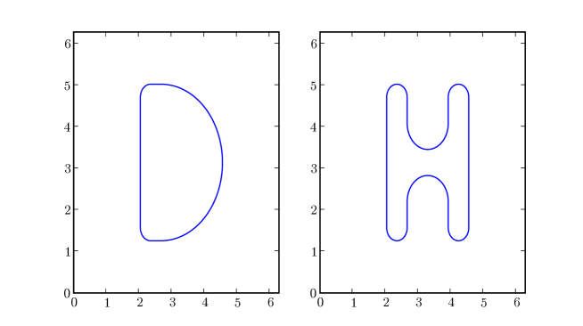
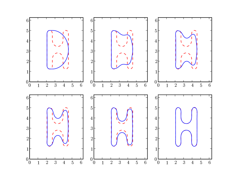
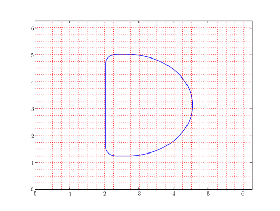
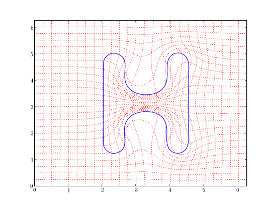
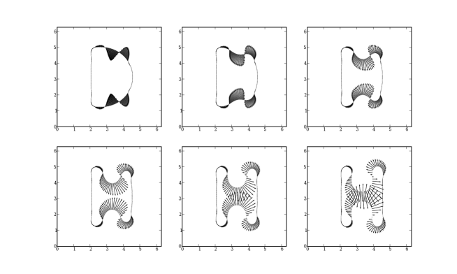
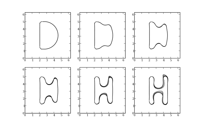
A plot of the two curves used for the tests is given in figure 1. These two curves are quite different and require large deformations to transform one curve into the other. The calculated path is illustrated in figure 2 with a few snapshots of the curve during the transformation at various times. The effect of the deforming flow on the surrounding space is illustrated in figure 3.

To illustrate the results of section 3.5, a plot showing momentum vectors at various times is given in figure 4 which suggests that the momentum stays normal to the curve. This is confirmed by figure 5, showing the evolution of $J_{\beta}\Delta\bi{Q}_{\beta}(0)$ which is an approximation to $\partial\bi{Q}/\partial s\rmd s$. The quantity $\sum_{\beta}\bi{P}_{\beta}\cdot J_{\beta}\Delta\bi{Q}_{\beta}$ remains within round-off error of zero throughout, confirming the results of section 3.5.

6 Summary and outlook

In this paper we introduced a new particle-mesh discretisation for diffeomorphic matching of curves, which can also be used for matching images. In this method the vector fields used to transport the curves are represented on a fixed mesh, whilst the curves themselves are represented by a finite set of moving points. Since the discrete equations arise from discretising an action principle, they are variational integrators which have many favourable properties. As discussed in [MM06a], whilst the benefits of variational integrators have been established for long integrations such as those for celestial mechanics or molecular dynamics, the benefits for short time optimal control problems such as the curve matching problem discussed in this paper are not so clear. There are a number of drawbacks and benefits which need to be investigated with further testing. In this paper we showed that the variational integrators that arise from the particle-mesh discretisation have a discrete form of the momentum conservation law which leads to the curve momentum remaining normal to the curve throughout the computed trajectory between shapes. We also noted that the integrators have a modified Hamiltonian which is conserved over long times (but not exponentially long since the compactly supported basis functions $\psi_{k}(\bi{x})$ are not analytic) which can be interpreted as a modified metric for the discrete equations. We then showed illustrative examples obtained from the calculation of the optimal trajectory between two closed curves in the plane.

The main computational challenge for diffeomorphic matching remains the design of efficient algorithms to obtain optimal trajectories for large datasets. Of the two solution methods described in section 4, the inexact matching method applied to the particle-mesh discretisation may be best applied in parallel by using a Newton-Krylov method to solve the Euler-Lagrange equations (including the penalty term) since it is possible to obtain a good initial guess for the optimal path by other methods. The minimisation-by-shooting approach might be best applied using a multilevel scheme where the problem is first solved with a small number of particles, with more particles being introduced once the lower dimensional problem has been solved to sufficient accuracy. These approaches will need to be developed in order for the discretisation to be applied to practical engineering applications, as well as convergence studies and error estimates.

In future work we shall investigate the convergence properties of this method in the limit as the number of points in the discretisation of the curve goes to infinity (together with the number of mesh points), and apply the method to investigate practical datasets.

Although we do not compute examples here, this method could also be used for matching surfaces in three dimensions using a current-matching approach. The main modifications are that equation (10) needs to be evaluated in three dimensions using a tensor product of three B-splines (one for each Cartesian component), and the parameterisation of the surface should become a triangulation with a singular current being interpolated from the surface to a three-dimensional mesh using the same basis functions. We will develop and investigate such a method in future work. We will also investigate efficiency of the particle-mesh versus the mesh-free fast multipoles approach of [VG05] in numerical tests on real data.

Further developments will be to apply the particle mesh to the related problem of metamorphosis [TY04], and to problems where quantities such as vector and tensor fields associated with images also need to be matched together.

References

- [Ber82] D. P. Bertsekas. Constrained Optimization and Lagrange Multiplier Methods. Academic Press, 1982.
- [BMTY05] M. F. Beg, M. I. Miller, A. Trouvé, and L. Younes. Computing large deformation metric mappings via geodesics flows of diffeomorphisms. International Journal Of Computer Vision, 61(2):139–157, 2005.
- [CH] C. J. Cotter and D. D. Holm. Continuous and discrete Clebsch variational principles. To appear in Foundations of Computational Mechanics, 2008.
- [CH93] R. Camassa and D. D. Holm. An integrable shallow water equation with peaked solitons. Phys. Rev. Lett., 71:1661–1664, 1993.
- [CH08] C. J. Cotter and D. D. Holm. Discrete momentum maps for lattice EPDiff. To appear in Handbook of Numerical Analysis, 2008.
- [CHH07] C. J. Cotter, D. D. Holm, and P. E. Hydon. Multisymplectic formulation of fluid dynamics using the inverse map. Proc. Roy. Soc. A, 463(2086):2671–2687, 2007.
- [Cot05] C. J. Cotter. A general approach for producing Hamiltonian numerical schemes for fluid equations. arXiv:math.NA/0501468, 2005.
- [CY01] V. Camion and L. Younes. Geodesic interpolating splines. In M Figueiredo, J Zerubia, and K Jain, A, editors, EMMCVPR 2001, volume 2134 of Lecture notes in computer sciences. Springer, 2001.
- [FGR02] J. Frank, G. Gottwald, and S. Reich. A Hamiltonian particle-mesh method for the rotating shallow-water equations. In Lecture Notes in Computational Science and Engineering, volume 26, pages 131–142. Springer-Verlag, 2002.
- [GM98] U. Grenander and M. I. Miller. Computational anatomy: An emerging discipline. Quarterly of Applied Mathematics, LVI(4):617–694, 1998.
- [GS91] L. Greengard and J. Strain. The fast Gauss transform. SIAM Journal of Scientific Statistical Computing, 12(79–94), 1991.
- [GTY04] J. Glaunes, A. Trouvé, and L. Younes. Diffeomorphic matching of distributions: A new approach for unlabelled point-sets and sub-manifolds matching. In IEEE Computer Society Conference on Computer Vision and Pattern Recognition, volume 2, pages 712–718, 2004.
- [GTY06] J. Glaunes, A. Trouve, and L. Younes. Modeling planar shape variation via hamiltonian flows of curves. In H. Krim and A. Yezzi Jr., editors, Statistics and Analysis of Shapes. Birkhäuser, 2006.
- [Gun03] M. D. Gunzburger. Perspectives in Flow Control and Optimization. Advances in design and control. SIAM, Philadelphia, USA, 2003.
- [HM04] D. D. Holm and J. E. Marsden. Momentum maps & measure valued solutions of the Euler-Poincaré equations for the diffeomorphism group. Progr. Math., 232:203–235, 2004. http://arxiv.org/abs/nlin.CD/0312048.
- [HMR98] D. D. Holm, J. E. Marsden, and T. S. Ratiu. The Euler–Poincaré equations and semidirect products with applications to continuum theories. Adv. in Math., 137:1–81, 1998. http://xxx.lanl.gov/abs/chao-dyn/9801015.
- [JMOB05] O. Junge, J. Marsden, and S. Ober-Blobaum. Discrete mechanics and optimal control. In Proceedings of the 16th IFAC World Congress, 2005.
- [JOP+ ] Eric Jones, Travis Oliphant, Pearu Peterson, et al. SciPy: Open source scientific tools for Python, 2001–. http://www.scipy.org/.
- [LMOW03] A. Lew, J. E. Marsden, M. Ortiz, and M. West. An overview of variational integrators. In L.P. Franca, editor, Finite Element Methods: 1970s and Beyond, pages 85–146. CIMNE, Barcelona, Spain, 2003.
- [LR05] B. Leimkuhler and S. Reich. Simulating Hamiltonian Dynamics. CUP, 2005.
- [MM06a] R. McLachlan and S. Marsland. Discrete mechanics and optimal control for image registration. ANZIAM Journal, 48, 2006.
- [MM06b] R. I. McLachlan and S. Marsland. The Kelvin-Helmholtz instability of momentum sheets in the Euler equations for planar diffeomorphisms. SIAM Journal on Applied Dynamical Systems, 5(4):726–758, 2006.
- [MMS06] A Mills, S Marsland, and T Shardlow. Biomedical Image Registration, chapter Computing the Geodesic Interpolating Spline. Number 169–177. Springer, 2006.
- [MTY03] M. I. Miller, A. Trouvé, and L. Younes. Geodesic shooting in computational anatomy. Technical report, Center for Imaging Science, Johns Hopkins University, 2003.
- [MY01] M. I. Miller and L. Younes. Group action, diffeomorphism and matching: a general framework. Int. J. Comp. Vis., 41:61–84, 2001.
- [TMT02] C. Twinings, S. Marsland, and C. Taylor. Measuring geodesic distances on the space of bounded diffeomorphisms. In British Macine Vision Conference, 2002.
- [TY04] A Trouvé and L Younes. Metamorphoses through lie group action. Technical report, Center for Imaging Science, Johns Hopkins University, 2004.
- [VG05] Marc Vaillant and Joan Glaunes. Surface matching via currents. In IPMI, pages 381–392, 2005.