Non-Markovian diffusion equations and processes:
analysis and simulations

Antonio MURA1, Murad S. TAQQU2 and Francesco MAINARDI1

1.11. Department of Physics, University of Bologna, and INFN, Via Irnerio 46, I-40126 Bologna, Italy

URL: http:// www.fracalmo.org

2.22. Department of Mathematics, Boston University, Boston, MA 02215, USA

URL: http://math.bu.edu/people/murad/


Revised Version: May 2008

in press on Physica A (2008), doi:10.1016/j.physa.2008.04.035


Keywords: Non-Markovian processes, fractional derivatives, anomalous diffusion, subordination, fractional Brownian motion.

Abstract: In this paper we introduce and analyze a class of diffusion type equations related to certain non-Markovian stochastic processes. We start from the forward drift equation which is made non-local in time by the introduction of a suitable chosen memory kernel K​(t)𝐾𝑑K(t). The resulting non-Markovian equation can be interpreted in a natural way as the evolution equation of the marginal density function of a random time process l​(t)𝑙𝑑l(t). We then consider the subordinated process Y​(t)=X​(l​(t))π‘Œπ‘‘π‘‹π‘™π‘‘Y(t)=X(l(t)) where X​(t)𝑋𝑑X(t) is a Markovian diffusion. The corresponding time evolution of the marginal density function of Y​(t)π‘Œπ‘‘Y(t) is governed by a non-Markovian Fokker-Planck equation which involves the memory kernel K​(t)𝐾𝑑K(t). We develop several applications and derive the exact solutions. We consider different stochastic models for the given equations providing path simulations.

1 Introduction

In this introduction, we describe and motivate the themes developed in the paper. Historical notes will be presented in Section 2.

Brownian motion B​(t)𝐡𝑑B(t), tβ‰₯0𝑑0t\geq 0, is a stochastic process with many properties. It is at the same time Gaussian and Markovian, has stationary increments and is self-similar. A process X​(t)𝑋𝑑X(t), tβ‰₯0𝑑0t\geq 0, is said to be self-similar with self-similarity exponent H𝐻H if, for all aβ‰₯0π‘Ž0a\geq 0, the processes X​(a​t)π‘‹π‘Žπ‘‘X(at), tβ‰₯0𝑑0t\geq 0, and aH​X​(t)superscriptπ‘Žπ»π‘‹π‘‘a^{H}X(t), tβ‰₯0𝑑0t\geq 0, have the same finite-dimensional distributions. Brownian motion is self-similar with exponent H=1/2𝐻12H=1/2. In contrast, fractional Brownian motion BH​(t)subscript𝐡𝐻𝑑B_{H}(t), tβ‰₯0𝑑0t\geq 0, is Gaussian, has stationary increments, is self-similar with self-similarity exponent 0<H<10𝐻10<H<1, but is not Markovian, unless H=1/2𝐻12H=1/2, in which case the fractional Brownian motion becomes Brownian motion. When 1/2<H<112𝐻11/2<H<1, the increments of fractional Brownian motion have long-range dependence [49].

Because Brownian motion is Markovian with stationary increments, its finite-dimensional distributions can be obtained from the marginal density function

fB​(x,t)=14​π​t​eβˆ’x2/4​t,xβˆˆβ„formulae-sequencesubscript𝑓𝐡π‘₯𝑑14πœ‹π‘‘superscript𝑒superscriptπ‘₯24𝑑π‘₯ℝf_{B}(x,t)=\frac{1}{\sqrt{4\pi t}}e^{-x^{2}/4t},\;\;x\in\mathbb{R} (1)

at time tβ‰₯0𝑑0t\geq 0. This density function is the fundamental solution of the β€œstandard” diffusion equation:

βˆ‚tu​(x,t)=βˆ‚x​xu​(x,t),subscript𝑑𝑒π‘₯𝑑subscriptπ‘₯π‘₯𝑒π‘₯𝑑\partial_{t}u(x,t)=\partial_{xx}u(x,t), (2)

which in integral form reads:

u​(x,t)=u0​(x)+∫0tβˆ‚x​xu​(x,s)​d​s,u0​(x)=u​(x,0).formulae-sequence𝑒π‘₯𝑑subscript𝑒0π‘₯superscriptsubscript0𝑑subscriptπ‘₯π‘₯𝑒π‘₯𝑠𝑑𝑠subscript𝑒0π‘₯𝑒π‘₯0u(x,t)=u_{0}(x)+\int_{0}^{t}\partial_{xx}u(x,s)ds,\;\;u_{0}(x)=u(x,0). (3)

Thus, fB​(x,t)subscript𝑓𝐡π‘₯𝑑f_{B}(x,t) is a solution of Eq. (3) with u0​(x)=δ​(x)subscript𝑒0π‘₯𝛿π‘₯u_{0}(x)=\delta(x), where δ​(x)𝛿π‘₯\delta(x) is the Dirac delta distribution. We allow, throughout the paper, functions to be distributions.

Remark 1.1.

We follow the physics convention of not including the factor 1/2121/2 in Eq. (2). Therefore, in this paper, β€œstandard” Brownian motion B​(t)𝐡𝑑B(t), tβ‰₯0𝑑0t\geq 0, is such that, for each time tβ‰₯0𝑑0t\geq 0, B​(t)∼N​(0,2​t)similar-to𝐡𝑑𝑁02𝑑B(t)\sim N(0,2t). The β€œtilde” notation X∼fX​(x)similar-to𝑋subscript𝑓𝑋π‘₯X\sim f_{X}(x) indicates that the random variable X𝑋X has the probability density function fX​(x)subscript𝑓𝑋π‘₯f_{X}(x).

Our goal is to extend Eq. (3) to non-Markovian settings. We will consider non-local, fractional and stretched modifications of the diffusion equation. These modified equations will be called Non-Markovian diffusion equations, because, while they originate from a diffusion equation, the corresponding process, whose probability density function is a solution of these modified equations, will be typically non-Markovian.

To motivate the modifications, consider first the non-random process l​(t)=t𝑙𝑑𝑑l(t)=t, tβ‰₯0𝑑0t\geq 0, which depicts a non-random linear time evolution and let fl​(Ο„,t)subscriptπ‘“π‘™πœπ‘‘f_{l}(\tau,t) denote its density function at time t𝑑t. Therefore one has fl​(Ο„,t)=δ​(Ο„βˆ’t)subscriptπ‘“π‘™πœπ‘‘π›Ώπœπ‘‘f_{l}(\tau,t)=\delta(\tau-t) where δ​(x)𝛿π‘₯\delta(x) is the Dirac distribution. It is natural to interpret fl​(Ο„,t)subscriptπ‘“π‘™πœπ‘‘f_{l}(\tau,t) as the fundamental solution of the standard forward drift equation:

βˆ‚tu​(Ο„,t)=βˆ’βˆ‚Ο„u​(Ο„,t),Ο„,tβ‰₯0,formulae-sequencesubscriptπ‘‘π‘’πœπ‘‘subscriptπœπ‘’πœπ‘‘πœπ‘‘0\partial_{t}u(\tau,t)=-\partial_{\tau}u(\tau,t),\;\;\tau,t\geq 0, (4)

which in integral form reads:

u​(Ο„,t)=u0​(Ο„)βˆ’βˆ«0tβˆ‚Ο„u​(Ο„,s)​d​s,u0​(Ο„)=u​(Ο„,0).formulae-sequenceπ‘’πœπ‘‘subscript𝑒0𝜏superscriptsubscript0𝑑subscriptπœπ‘’πœπ‘ π‘‘π‘ subscript𝑒0πœπ‘’πœ0u(\tau,t)=u_{0}(\tau)-\int_{0}^{t}\partial_{\tau}u(\tau,s)ds,\;\;\;u_{0}(\tau)=u(\tau,0). (5)

The general solutions are of the form u​(Ο„,t)=u0​(Ο„βˆ’t)π‘’πœπ‘‘subscript𝑒0πœπ‘‘u(\tau,t)=u_{0}(\tau-t) and thus, when u0​(Ο„)=δ​(Ο„)subscript𝑒0πœπ›Ώπœu_{0}(\tau)=\delta(\tau), the solution of Eq. (4) is indeed u​(Ο„,t)=δ​(Ο„βˆ’t)π‘’πœπ‘‘π›Ώπœπ‘‘u(\tau,t)=\delta(\tau-t). Observe that the variable Ο„β‰₯0𝜏0\tau\geq 0 plays the role of a space variable.

We will consider the following generalization of the forward drift equation (5)

u​(Ο„,t)=u0​(Ο„)βˆ’βˆ«0tK​(tβˆ’s)β€‹βˆ‚Ο„u​(Ο„,s)​d​s,Ο„,tβ‰₯0,formulae-sequenceπ‘’πœπ‘‘subscript𝑒0𝜏superscriptsubscript0𝑑𝐾𝑑𝑠subscriptπœπ‘’πœπ‘ π‘‘π‘ πœπ‘‘0u(\tau,t)=u_{0}(\tau)-\int_{0}^{t}K(t-s)\partial_{\tau}u(\tau,s)ds,\;\;\tau,t\geq 0, (6)

where K​(t)𝐾𝑑K(t), with tβ‰₯0𝑑0t\geq 0, is a suitable kernel chosen such that the fundamental solution of Eq. (6) is a probability density function at each tβ‰₯0𝑑0t\geq 0. We refer to Eq. (6) as the non-Markovian forward drift equation.

The presence of the memory kernel K𝐾K in Eq. (6) suggests a corresponding modification of the diffusion equation (3). Namely, we will consider the equation:

u​(x,t)=u0​(x)+∫0tK​(tβˆ’s)β€‹βˆ‚x​xu​(x,s)​d​s,xβˆˆβ„,tβ‰₯0.formulae-sequence𝑒π‘₯𝑑subscript𝑒0π‘₯superscriptsubscript0𝑑𝐾𝑑𝑠subscriptπ‘₯π‘₯𝑒π‘₯𝑠𝑑𝑠formulae-sequenceπ‘₯ℝ𝑑0u(x,t)=u_{0}(x)+\int_{0}^{t}K(t-s)\partial_{xx}u(x,s)ds,\;\;x\in\mathbb{R},\;\;t\geq 0. (7)

Its fundamental solution turns out to be:

f​(x,t)=∫0∞G​(x,Ο„)​h​(Ο„,t)​𝑑τ,𝑓π‘₯𝑑superscriptsubscript0𝐺π‘₯πœβ„Žπœπ‘‘differential-d𝜏f(x,t)=\int_{0}^{\infty}G(x,\tau)h(\tau,t)d\tau, (8)

where

G​(x,t)=14​π​t​exp⁑(βˆ’x2/4​t),𝐺π‘₯𝑑14πœ‹π‘‘superscriptπ‘₯24𝑑G(x,t)=\frac{1}{\sqrt{4\pi t}}\exp(-x^{2}/4t), (9)

and h​(Ο„,t)β„Žπœπ‘‘h(\tau,t) is the fundamental solution of Eq. (6).

The solution (8) is a marginal (one-point) probability density function. We will consider different random processes whose marginal probability density function coincides with it. As illustration, consider the following examples111In these examples we refer to facts which are justified later in the paper through forward references. The reader may want to focus at this point only on the examples and ignore the references..

Example 1.1.

If we choose:

K​(t)=tβˆ’1/2Ο€,tβ‰₯0,formulae-sequence𝐾𝑑superscript𝑑12πœ‹π‘‘0K(t)=\frac{t^{-1/2}}{\sqrt{\pi}},\;\;t\geq 0, (10)

then we have, see Eq. (65 and Eq. (70):

h​(Ο„,t)=1π​t​exp⁑(βˆ’Ο„24​t),Ο„β‰₯0,tβ‰₯0,formulae-sequenceβ„Žπœπ‘‘1πœ‹π‘‘superscript𝜏24𝑑formulae-sequence𝜏0𝑑0h(\tau,t)=\frac{1}{\sqrt{\pi t}}\exp\left(-\frac{\tau^{2}}{4t}\right),\;\;\tau\geq 0,\;\;t\geq 0, (11)

as the fundamental solution of Eq. (6). Now consider the process

D​(t)=B​(l​(t)),tβ‰₯0,formulae-sequence𝐷𝑑𝐡𝑙𝑑𝑑0D(t)=B(l(t)),\;\;t\geq 0, (12)

where B𝐡B is a β€œstandard” Brownian motion and l​(t)β‰₯0𝑙𝑑0l(t)\geq 0 is a random time-change (not necessarily increasing), independent of B𝐡B, whose marginal density function is given by h​(Ο„,t)β„Žπœπ‘‘h(\tau,t). One possible choice for the random time process is simply:

l​(t)=|b​(t)|,tβ‰₯0,formulae-sequence𝑙𝑑𝑏𝑑𝑑0l(t)=|b(t)|,\;\;t\geq 0,

where b​(t)𝑏𝑑b(t), tβ‰₯0𝑑0t\geq 0, is a β€œstandard” Brownian motion [9, 18]. Such a random time process l​(t)𝑙𝑑l(t), tβ‰₯0𝑑0t\geq 0, is self-similar of order H=1/2𝐻12H=1/2.222 Another possible choice for a random time process with marginal density given by Eq. (11) is the local time in zero of a β€œstandard” Brownian motion [4]. In this case the time-change process l​(t)𝑙𝑑l(t) is increasing. Let now B​(t)𝐡𝑑B(t), tβ‰₯0𝑑0t\geq 0, be another β€œstandard” Brownian motion independent of b​(t)𝑏𝑑b(t). Thus, the process (see also [3])

D​(t)=B​(|b​(t)|),tβ‰₯0,formulae-sequence𝐷𝑑𝐡𝑏𝑑𝑑0D(t)=B(|b(t)|),\;\;t\geq 0, (13)

has marginal density defined by Eq. (8) with h​(Ο„,t)β„Žπœπ‘‘h(\tau,t) given by Eq. (11).

But, D​(t)𝐷𝑑D(t) is not the only process with density function f​(x,t)𝑓π‘₯𝑑f(x,t), given by Eq. (8). For example, the process

Y​(t)=|b​(1)|​B1/4​(t),tβ‰₯0,formulae-sequenceπ‘Œπ‘‘π‘1subscript𝐡14𝑑𝑑0Y(t)=\sqrt{|b(1)|}B_{1/4}(t),\;\;t\geq 0\,, (14)

where B1/4subscript𝐡14B_{1/4} is an independent fractional Brownian motion with self-similarity exponent H=1/4𝐻14H=1/4, has the same one-dimensional probability density functions as the previous process D​(t)𝐷𝑑D(t), tβ‰₯0𝑑0t\geq 0, see Eq. (40) with Ξ²=1/2𝛽12\beta=1/2.

Example 1.2.

The fractional Brownian motion in Eq. (14) has a self-similarity exponent H<1/2𝐻12H<1/2. The increments of such a process are known to be negatively correlated [31, 32, 49]. To allow for the presence of fractional Brownian motion BH​(t)subscript𝐡𝐻𝑑B_{H}(t) with 0<H<10𝐻10<H<1, we introduce a second (non-random) time-change tβ†’g​(t)→𝑑𝑔𝑑t\rightarrow g(t), where g​(0)=0𝑔00g(0)=0 and g​(t)𝑔𝑑g(t) is smooth and increasing, that is we consider the non-Markovian diffusion equation

u​(x,t)=u0​(x)+∫0tg′​(s)​K​(g​(t)βˆ’g​(s))β€‹βˆ‚x​xu​(x,s)​d​s.𝑒π‘₯𝑑subscript𝑒0π‘₯superscriptsubscript0𝑑superscript𝑔′𝑠𝐾𝑔𝑑𝑔𝑠subscriptπ‘₯π‘₯𝑒π‘₯𝑠𝑑𝑠u(x,t)=u_{0}(x)+\int_{0}^{t}g^{\prime}(s)K\left(g(t)-g(s)\right)\partial_{xx}u(x,s)ds. (15)

whose fundamental solution is now:

f​(x,t)=∫0∞G​(x,Ο„)​h​(Ο„,g​(t))​𝑑τ,𝑓π‘₯𝑑superscriptsubscript0𝐺π‘₯πœβ„Žπœπ‘”π‘‘differential-d𝜏f(x,t)=\int_{0}^{\infty}G(x,\tau)h(\tau,g(t))d\tau, (16)

where hβ„Žh is the fundamental solution of Eq. (6). If K​(t)𝐾𝑑K(t) is as in Eq. (10) and g​(t)=t2​α𝑔𝑑superscript𝑑2𝛼g(t)=t^{2\alpha}, with 0<Ξ±<20𝛼20<\alpha<2, then the processes:

D​(t)=B​(|b​(t2​α)|),tβ‰₯0,Y​(t)=|b​(1)|​BΞ±/2​(t),tβ‰₯0,formulae-sequence𝐷𝑑𝐡𝑏superscript𝑑2𝛼𝑑0missing-subexpressionformulae-sequenceπ‘Œπ‘‘π‘1subscript𝐡𝛼2𝑑𝑑0missing-subexpression\begin{array}[]{ll}D(t)=B(|b(t^{2\alpha})|),\;\;t\geq 0,\\[8.5359pt] Y(t)=\sqrt{|b(1)|}B_{\alpha/2}(t),\;\;t\geq 0,\end{array}

have a marginal density function defined by Eq. (16) with h​(Ο„,t)β„Žπœπ‘‘h(\tau,t) as in Eq. (11), which is the fundamental solution of Eq. (15). In this case Y​(t)π‘Œπ‘‘Y(t) is defined through an independent fractional Brownian motion BΞ±/2subscript𝐡𝛼2B_{\alpha/2} with Hurst’s parameter H=Ξ±/2𝐻𝛼2H=\alpha/2 and thus 0<H<10𝐻10<H<1. This is a special case of Eq. (78).

The preceding examples illustrate the themes pursued in the paper. We will focus, however, not only on power-like kernels such as those defined in Eq. (10), but also on exponential-like kernels such as:

K​(t)=eβˆ’a​t,aβ‰₯0.formulae-sequence𝐾𝑑superscriptπ‘’π‘Žπ‘‘π‘Ž0K(t)=e^{-at},\;\;a\geq 0. (17)

We also consider what happens when the Brownian motion B​(t)𝐡𝑑B(t), tβ‰₯0𝑑0t\geq 0, is replaced by a more general linear (time-homogeneous) diffusion Q​(t)𝑄𝑑Q(t), tβ‰₯0,𝑑0t\geq 0, governed by the Fokker-Planck equation333Also known as the forward Kolmogorov equation.,

βˆ‚tu​(x,t)=𝒫x​u​(x,t),subscript𝑑𝑒π‘₯𝑑subscript𝒫π‘₯𝑒π‘₯𝑑\partial_{t}u(x,t)=\mathcal{P}_{x}u(x,t), (18)

where 𝒫xsubscript𝒫π‘₯\mathcal{P}_{x} is a linear operator independent of t𝑑t acting on the variable xβˆˆβ„π‘₯ℝx\in\mathbb{R}. In other words we consider the non-Markovian diffusion equation:

u​(x,t)=u0​(x)+∫0tg′​(s)​K​(g​(t)βˆ’g​(s))​𝒫x​u​(x,s)​𝑑s.𝑒π‘₯𝑑subscript𝑒0π‘₯superscriptsubscript0𝑑superscript𝑔′𝑠𝐾𝑔𝑑𝑔𝑠subscript𝒫π‘₯𝑒π‘₯𝑠differential-d𝑠u(x,t)=u_{0}(x)+\int_{0}^{t}g^{\prime}(s)K(g(t)-g(s))\mathcal{P}_{x}u(x,s)ds. (19)

We show that its fundamental solution is:

f​(x,t)=∫0βˆžπ’’β€‹(x,Ο„)​h​(Ο„,g​(t))​𝑑τ,𝑓π‘₯𝑑superscriptsubscript0𝒒π‘₯πœβ„Žπœπ‘”π‘‘differential-d𝜏f(x,t)=\int_{0}^{\infty}\mathcal{G}(x,\tau)h(\tau,g(t))d\tau, (20)

where 𝒒​(x,t)𝒒π‘₯𝑑\mathcal{G}(x,t) is the fundamental solution of Eq. (19), while h​(Ο„,t)β„Žπœπ‘‘h(\tau,t) is the fundamental solution of Eq. (6). We also provide explicit solutions when 𝒫xsubscript𝒫π‘₯\mathcal{P}_{x} is the differential operator associated with Brownian motion with drift, when it is associated with Geometric Brownian motion and when the kernel K​(t)𝐾𝑑K(t) is the power kernel and the exponential kernel.

In order not to dwell on technicalities, we suppose implicitly, throughout the paper, that we have sufficient regularity conditions, to justify the algebraic manipulations that are performed. The paper is organized as follows:

  • β€’

    Historical notes are presented in Section 2.

  • β€’

    In Section 3 we study the non-Markovian forward drift equation (6) and its corresponding random time process l​(t)𝑙𝑑l(t). We derive suitability conditions on the kernel K​(t)𝐾𝑑K(t). We end the section by noting that a self-similar time-change process, for instance with self-similarity parameter H=β𝐻𝛽H=\beta, requires the choice K​(t)=C​tΞ²βˆ’1/Γ​(Ξ²)𝐾𝑑𝐢superscript𝑑𝛽1Γ𝛽K(t)=Ct^{\beta-1}/\Gamma(\beta) with 0<β≀10𝛽10<\beta\leq 1.

  • β€’

    In Section 4 we study the non-Markovian diffusion equation (15) and its solutions, and we discuss its various stochastic interpretations.

  • β€’

    In Section 5 we illustrate the fact that the stochastic representation is not unique.

  • β€’

    In Section 6 we study the more general non-Markovian Fokker-Planck equation and derive its solution Eq. (20).

  • β€’

    In Section 7 we go thorough several examples with 𝒫x​u​(x,t)=βˆ‚x​xu​(x,t)subscript𝒫π‘₯𝑒π‘₯𝑑subscriptπ‘₯π‘₯𝑒π‘₯𝑑\mathcal{P}_{x}u(x,t)=\partial_{xx}u(x,t), that is, when the underlying diffusion proces is Brownian motion. We consider non-Markovian diffusion equations, associated with the β𝛽\beta-power kernel K​(t)=tΞ²βˆ’1/Γ​(Ξ²)𝐾𝑑superscript𝑑𝛽1Γ𝛽K(t)=t^{\beta-1}/\Gamma(\beta), 0<β≀10𝛽10<\beta\leq 1, and with the exponential-decay kernel K​(t)=eβˆ’a​t𝐾𝑑superscriptπ‘’π‘Žπ‘‘K(t)=e^{-at}, aβ‰₯0π‘Ž0a\geq 0. We also consider different choices of the deterministic scaling function g​(t)𝑔𝑑g(t), for example a logarithmic time scale g​(t)=log⁑(t+1)𝑔𝑑𝑑1g(t)=\log(t+1) is considered.

  • β€’

    In Section 8 we focus on applications when the underlying diffusion process is not standard Brownian motion. We consider the case of Brownian motion with drift and Geometric Brownian motion and we study the corresponding equations with the β𝛽\beta-power kernel and the exponential-decay kernel.

  • β€’

    Section 9 contains a summary and concluding remarks.

2 Historical notes

Non-Markovian equations like Eq. (7), or more generally Eq. (19), are often encountered when studying physical phenomena related to relaxation and diffusion problems in complex systems (see Srokowsky [47] for examples).

Equations of the type (7) have been studied for example by Kolsrud [22]. He obtained Eq. 8), but without providing specific examples. A similar study was done by Wyss [51] who, however, focused only on power-like kernels K​(t)=C​tΞ²βˆ’1𝐾𝑑𝐢superscript𝑑𝛽1K(t)=Ct^{\beta-1}.

Sokolov [45] (see also Srokowsky [47]), studied the non-Markovian equation

βˆ‚tP​(x,t)=∫0tk​(tβˆ’s)​Lx​P​(x,s)​𝑑s,subscript𝑑𝑃π‘₯𝑑superscriptsubscript0π‘‘π‘˜π‘‘π‘ subscript𝐿π‘₯𝑃π‘₯𝑠differential-d𝑠\partial_{t}P(x,t)=\int_{0}^{t}k(t-s)L_{x}P(x,s)ds, (21)

where Lxsubscript𝐿π‘₯L_{x} is a linear operator acting on the variable xπ‘₯x. He provided a formal solution in the form of Eq. 20). Observe, however, that our equation (19) differs from Eq. (21), not only by the presence of the scaling function g​(t)𝑔𝑑g(t), but also by the choice of the memory kernel. Our kernel K​(t)𝐾𝑑K(t) and Sokolov’s kernel k​(t)π‘˜π‘‘k(t) are related by the equation:

K​(t)=∫0tk​(s)​𝑑sβ‡’K~​(s)=k~​(s)/s,s>0,formulae-sequence𝐾𝑑superscriptsubscript0π‘‘π‘˜π‘ differential-d𝑠⇒~𝐾𝑠~π‘˜π‘ π‘ π‘ 0K(t)=\int_{0}^{t}k(s)ds\Rightarrow\widetilde{K}(s)=\widetilde{k}(s)/s,\;\;s>0, (22)

where the tilde indicates the Laplace transform, see Eq. (25). The suitability conditions for these memory kernels are thus not the same (these conditions are developed in Section 3). For example, consider the simple exponential-decay kernel eβˆ’a​tsuperscriptπ‘’π‘Žπ‘‘e^{-at}, aβ‰₯0π‘Ž0a\geq 0. This choice of the kernel is β€œsafe” in the context of Eq. (19), i.e. for the choice K​(t)=eβˆ’a​t𝐾𝑑superscriptπ‘’π‘Žπ‘‘K(t)=e^{-at}, but is β€œdangerous” if one considers Eq. (21) with the kernel k​(t)=eβˆ’a​tπ‘˜π‘‘superscriptπ‘’π‘Žπ‘‘k(t)=e^{-at}. In the case of Eq. (19), the exponential-decay kernel corresponds to a system for which non-local memory effects are initially negligible. In fact, K​(t)=eβˆ’a​tβ†’1𝐾𝑑superscriptπ‘’π‘Žπ‘‘β†’1K(t)=e^{-at}\rightarrow 1 as tβ†’0→𝑑0t\rightarrow 0 and thus the system appears Markovian at small times. On the other hand, the choice k​(t)=eβˆ’a​tπ‘˜π‘‘superscriptπ‘’π‘Žπ‘‘k(t)=e^{-at} corresponds to the kernel K​(t)=aβˆ’1​(1βˆ’eβˆ’a​t)𝐾𝑑superscriptπ‘Ž11superscriptπ‘’π‘Žπ‘‘K(t)=a^{-1}(1-e^{-at}) which for small times behaves like t𝑑t. In this case Sokolov [45] noticed that the corresponding equations are only reasonable in a restricted domain of the model parameters and for certain initial and boundary conditions.

Our starting point is different from that of the previous authors. Instead of starting directly from the Fokker-Planck equations (18), we start from the forward drift equation (5) which is then generalized by introducing a memory kernel K​(t)𝐾𝑑K(t), Eq. (6). One is then naturally led to the non-Markovian diffusion equations (15 and (19) after the introduction of the scaling function g​(t)𝑔𝑑g(t). In fact, in specific cases, it is sometimes simpler to solve first the non-Markovian forward drift equation (6) and then use the solution to solve the non-Markovian diffusion equation (15) or (19) by using (16) or (20). The form of the solution (16) or (20) has now a ready-made interpretation. For example, in Eq. (20) the function 𝒒​(x,t)𝒒π‘₯𝑑\mathcal{G}(x,t) is the fundamental solution of the Markovian equation (18) and the function h​(Ο„,t)β„Žπœπ‘‘h(\tau,t) is the fundamental solution of the non-Markovian equation (6) and it is these two solutions that contribute to Eq. (20) which is the fundamental solution of the non-Markovian diffusion equation (19).

Furthermore, the form (16) or (20) has a natural interpretation in terms of subordinated processes, see Eq. (12). According to Whitmore and Lee [23], the term β€œsubordination” was introduced by Bochner [5, 6]. It refers to processes of the form Y​(t)=X​(l​(t))π‘Œπ‘‘π‘‹π‘™π‘‘Y(t)=X(l(t)), tβ‰₯0𝑑0t\geq 0, where X​(t)𝑋𝑑X(t), tβ‰₯0𝑑0t\geq 0, is a Markov process and l​(t)𝑙𝑑l(t), tβ‰₯0𝑑0t\geq 0, is a (non-negative) random time process independent of X𝑋X. The marginal distribution of the subordinated process is clearly:

fY​(x,t)=∫0∞fX​(x,Ο„)​fl​(Ο„,t)​𝑑τ,tβ‰₯0,xβˆˆβ„,formulae-sequencesubscriptπ‘“π‘Œπ‘₯𝑑superscriptsubscript0subscript𝑓𝑋π‘₯𝜏subscriptπ‘“π‘™πœπ‘‘differential-d𝜏formulae-sequence𝑑0π‘₯ℝf_{Y}(x,t)=\int_{0}^{\infty}f_{X}(x,\tau)f_{l}(\tau,t)d\tau,\;\;t\geq 0,\;\;x\in\mathbb{R}, (23)

where fX​(x,t)subscript𝑓𝑋π‘₯𝑑f_{X}(x,t) and fl​(Ο„,t)subscriptπ‘“π‘™πœπ‘‘f_{l}(\tau,t) represent the marginal density functions of the processes X𝑋X and l𝑙l. Therefore, Eq. (16) or Eq. (20) can be interpreted in terms of subordinated processes, with Eq. (6) characterizing the random time process l​(t)𝑙𝑑l(t) and Eq. (18) characterizing the Markov parent process X​(t)𝑋𝑑X(t).

The stochastic interpretation through subordinated processes, first suggested by Kolsrud, is very natural because Y​(t)=X​(l​(t))π‘Œπ‘‘π‘‹π‘™π‘‘Y(t)=X(l(t)) has a direct physical interpretation. For example, in equipment usage, X​(t)𝑋𝑑X(t) can be the state of a machine at time t𝑑t and l​(t)𝑙𝑑l(t) the effective usage up to time t𝑑t. In an econometric study, X​(t)𝑋𝑑X(t) may be a model for the price of a stock at time t𝑑t. If l​(t)𝑙𝑑l(t) measures the total economic activity up to time t𝑑t, the price of the stock at time t𝑑t should not be described by X​(t)𝑋𝑑X(t) but by the subordinated process Y​(t)=X​(l​(t))π‘Œπ‘‘π‘‹π‘™π‘‘Y(t)=X(l(t)). The resulting subordinated process Y​(t)π‘Œπ‘‘Y(t) is in general non-Markovian. In this way, the non-local memory effects are attributable to the random time process l​(t)𝑙𝑑l(t) and to its dynamics which is in general non-local in time, see Eq. (6).

Note, however, that the solution of Eq. (19) represents only the marginal (one-point) density function of the process and therefore cannot characterize the full stochastic structure of the process. As we note in the paper, there are also processes that are not subordinated processes that serve as stochastic models for non-Markovian diffusion equations like Eq. (19) or Eq. (21).

For example, consider in Eq. (7) the β𝛽\beta-power kernel K​(t)=tΞ²βˆ’1/Γ​(Ξ²)𝐾𝑑superscript𝑑𝛽1Γ𝛽K(t)=t^{\beta-1}/\Gamma(\beta), with 0<β≀10𝛽10<\beta\leq 1. From a stochastic point of view, the fundamental solution of this equation, also called the time-fractional diffusion equation of order β𝛽\beta, can be interpreted as the marginal density function of a self-similar stochastic processes with parameter H=Ξ²/2𝐻𝛽2H=\beta/2. This process, for example, can be taken to be a subordinated process Y​(t)=B​(l​(t))π‘Œπ‘‘π΅π‘™π‘‘Y(t)=B(l(t)), with a suitable choice of the random time l𝑙l. In Kolsrud [22], the random time l𝑙l is taken to be related to the local time of a d=2​(1βˆ’Ξ²)𝑑21𝛽d=2(1-\beta)-dimensional fractional Bessel process, while in Meerschaert et al. [34] (see also [1, 15, 16, 21, 40, 48, 17]), in the context of a Continuous Time Random Walk (CTRW), it is chosen to be the inverse of the totally skewed strictly β𝛽\beta-stable process. The interested reader is referred to the wide literature concerning the relationship between CTRW and non-Markovian diffusion equations and its applications. See for instance, [2, 13, 19, 35, 36, 42, 50, 52, 41, 28, 14] and references therein.

Schneider [43], moreover, in a very general mathematical construction, introduced the so-called Grey Brownian motion. This process is a self-similar process with stationary increments which, as turns out, can be represented by Y​(t)=Λβ​BH​(t)π‘Œπ‘‘subscriptΛ𝛽subscript𝐡𝐻𝑑Y(t)=\Lambda_{\beta}B_{H}(t), tβ‰₯0𝑑0t\geq 0, where BHsubscript𝐡𝐻B_{H} is a fractional Brownian motion with H=Ξ²/2𝐻𝛽2H=\beta/2 and ΛβsubscriptΛ𝛽\Lambda_{\beta} is a suitable chosen random variable independent of BHsubscript𝐡𝐻B_{H} (see Mura et al. for details [38, 39]). This process has a marginal density function that evolves in time according to the time-fractional diffusion equation of order β𝛽\beta. In this case the non-Markovian property is due to the presence of the fractional Brownian motion. As we show in the paper, long-range dependence can be made to appear through the time-scaling function g​(t)𝑔𝑑g(t), see Eq. (15) and Example 1.2. Figures 4, 5 and 6 display trajectories of the processes D​(t)𝐷𝑑D(t) and Y​(t)π‘Œπ‘‘Y(t) and corresponding density functions.

3 The non-Markovian forward drift equation

We start with the following generalization of Eq. (5), namely:

u​(Ο„,t)=u0​(Ο„)βˆ’βˆ«0tK​(tβˆ’s)β€‹βˆ‚Ο„u​(Ο„,s)​d​s,Ο„,tβ‰₯0,formulae-sequenceπ‘’πœπ‘‘subscript𝑒0𝜏superscriptsubscript0𝑑𝐾𝑑𝑠subscriptπœπ‘’πœπ‘ π‘‘π‘ πœπ‘‘0u(\tau,t)=u_{0}(\tau)-\int_{0}^{t}K(t-s)\partial_{\tau}u(\tau,s)ds,\;\;\tau,t\geq 0, (24)

where K​(t)𝐾𝑑K(t), with tβ‰₯0𝑑0t\geq 0, is a suitable chosen kernel. We then choose a random time process l​(t)𝑙𝑑l(t) such that, for each tβ‰₯0𝑑0t\geq 0, its marginal density fl​(Ο„,t)subscriptπ‘“π‘™πœπ‘‘f_{l}(\tau,t) is the fundamental solution of Eq. (24). Observe that Eq. (24) is β€œnon-local” because u​(Ο„,t)π‘’πœπ‘‘u(\tau,t) involves u​(Ο„,s)π‘’πœπ‘ u(\tau,s) at all 0≀s≀t0𝑠𝑑0\leq s\leq t. Equation (24) will be called non-Markovian forward drift equation, see Section 1, Eq. (6).

It is convenient to work with Laplace transforms. We indicate by ℒ​{φ​(x,t);t,s}β„’πœ‘π‘₯𝑑𝑑𝑠\mathscr{L}\{\varphi(x,t);t,s\} the Laplace transform of the function Ο†πœ‘\varphi with respect to t𝑑t evaluated in sβ‰₯0𝑠0s\geq 0, namely:

ℒ​{φ​(x,t);t,s}=∫0∞eβˆ’t​s​φ​(x,t)​𝑑t,sβ‰₯0.formulae-sequenceβ„’πœ‘π‘₯𝑑𝑑𝑠superscriptsubscript0superscriptπ‘’π‘‘π‘ πœ‘π‘₯𝑑differential-d𝑑𝑠0\mathscr{L}\{\varphi(x,t);t,s\}=\int_{0}^{\infty}e^{-ts}\varphi(x,t)dt,\;\;s\geq 0. (25)

If the function Ο†πœ‘\varphi depends only on the variable t𝑑t we write simply Ο†~​(s)~πœ‘π‘ \widetilde{\varphi}(s), because in this case there is no ambiguity concerning the integration variable. In particular we let K~​(s)~𝐾𝑠\widetilde{K}(s) denote the Laplace transform of the kernel K𝐾K.

Proposition 3.1.

Let fl​(Ο„,t)subscriptπ‘“π‘™πœπ‘‘f_{l}(\tau,t) denote the fundamental solution of Eq. (24). Then,

ℒ​{fl​(Ο„,t);t,s}=1s​K~​(s)​exp⁑(βˆ’Ο„K~​(s)),Ο„,sβ‰₯0,formulae-sequenceβ„’subscriptπ‘“π‘™πœπ‘‘π‘‘π‘ 1𝑠~πΎπ‘ πœ~πΎπ‘ πœπ‘ 0\mathscr{L}\{f_{l}(\tau,t);t,s\}=\frac{1}{s\widetilde{K}(s)}\exp{\left(-\frac{\tau}{\widetilde{K}(s)}\right)},\;\;\tau,s\geq 0, (26)

and zero for Ο„<0𝜏0\tau<0.

Proof: we take the Laplace transform with respect to the variable t𝑑t in Eq. (24):

βˆ‚Ο„u~​(Ο„,s)=u0​(Ο„)s​K~​(s)βˆ’u~​(Ο„,s)K~​(s),subscript𝜏~π‘’πœπ‘ subscript𝑒0πœπ‘ ~𝐾𝑠~π‘’πœπ‘ ~𝐾𝑠\partial_{\tau}\widetilde{u}(\tau,s)=\frac{u_{0}(\tau)}{s\widetilde{K}(s)}-\frac{\widetilde{u}(\tau,s)}{\widetilde{K}(s)}, (27)

thus Eq. (26) is a solution, in the distributional sense, when u0​(Ο„)=δ​(Ο„)subscript𝑒0πœπ›Ώπœu_{0}(\tau)=\delta(\tau). Indeed the general solution ofEq. 27) with u0​(Ο„)=δ​(Ο„)subscript𝑒0πœπ›Ώπœu_{0}(\tau)=\delta(\tau) is:

φ​(Ο„,s)=θ​(Ο„)s​K~​(s)​exp⁑(βˆ’Ο„K~​(s))+C​exp⁑(βˆ’Ο„K~​(s)),Ο„βˆˆβ„,formulae-sequenceπœ‘πœπ‘ πœƒπœπ‘ ~πΎπ‘ πœ~πΎπ‘ πΆπœ~πΎπ‘ πœβ„\varphi(\tau,s)=\frac{\theta(\tau)}{s\widetilde{K}(s)}\exp{\left(-\frac{\tau}{\widetilde{K}(s)}\right)}+C\exp{\left(-\frac{\tau}{\widetilde{K}(s)}\right)},\;\;\;\tau\in\mathbb{R},

where C𝐢C is a real constant and where

θ​(x)={1,xβ‰₯0,0,x<0πœƒπ‘₯cases1π‘₯00π‘₯0\theta(x)=\left\{\begin{array}[]{ll}1,&x\geq 0,\\ 0,&x<0\end{array}\right. (28)

is the Heaviside’s step function. Since we require φ​(Ο„,t)=0πœ‘πœπ‘‘0\varphi(\tau,t)=0 for Ο„<0𝜏0\tau<0, we get C=0𝐢0C=0 i.e. Eq. (26). β–‘β–‘\Box

3.1 Suitability conditions on the kernel K𝐾K

We must choose the kernel K𝐾K such that the fundamental solution of Eq. (24) is a probability density in Ο„β‰₯0𝜏0\tau\geq 0. We observe that if fl​(Ο„,t)subscriptπ‘“π‘™πœπ‘‘f_{l}(\tau,t) satisfies Eq. (24) and Eq. (26), then it is automatically normalized for each tβ‰₯0𝑑0t\geq 0. In fact, for a function φ​(x,t)πœ‘π‘₯𝑑\varphi(x,t) for which it is always possible to change the order of integration, one has:

βˆ«β„Ο†β€‹(x,t)​𝑑x=1βŸΊβˆ«β„Ο†~​(x,s)​𝑑x=sβˆ’1.⟺subscriptβ„πœ‘π‘₯𝑑differential-dπ‘₯1subscriptℝ~πœ‘π‘₯𝑠differential-dπ‘₯superscript𝑠1\int_{\mathbb{R}}\varphi(x,t)dx=1\Longleftrightarrow\int_{\mathbb{R}}\widetilde{\varphi}(x,s)dx=s^{-1}. (29)

Since Eq. (26) satisfies the right-hand side of Eq. (29), we get βˆ«β„+fl​(Ο„,t)​𝑑τ=1subscriptsubscriptℝsubscriptπ‘“π‘™πœπ‘‘differential-d𝜏1\int_{\mathbb{R}_{+}}f_{l}(\tau,t)d\tau=1. One still needs, however, to choose the kernel K𝐾K such that fl​(Ο„,t)β‰₯0subscriptπ‘“π‘™πœπ‘‘0f_{l}(\tau,t)\geq 0 for all Ο„,tβ‰₯0πœπ‘‘0\tau,t\geq 0.

In order to get a suitable condition on the kernel K𝐾K, we make use of the notion of completely monotone function. Recall that a function φ​(t)πœ‘π‘‘\varphi(t) is completely monotone if it is non-negative and possesses derivatives of any order and:

(βˆ’1)k​dkd​tk​φ​(t)β‰₯0,t>0,kβˆˆβ„€+={0,1,2,…}.formulae-sequencesuperscript1π‘˜superscriptπ‘‘π‘˜π‘‘superscriptπ‘‘π‘˜πœ‘π‘‘0formulae-sequence𝑑0π‘˜subscriptβ„€012…(-1)^{k}\frac{d^{k}}{dt^{k}}\varphi(t)\geq 0,\;\;\;t>0,\;\;k\in\mathbb{Z}_{+}=\{0,1,2,\dots\}. (30)

We observe that as tβ†’0→𝑑0t\rightarrow 0, the limit of dk​φ​(t)/d​tksuperscriptπ‘‘π‘˜πœ‘π‘‘π‘‘superscriptπ‘‘π‘˜d^{k}\varphi(t)/dt^{k} may be finite or infinite. Typical non-trivial examples are φ​(t)=exp⁑(βˆ’a​t)πœ‘π‘‘π‘Žπ‘‘\varphi(t)=\exp(-at), with a>0π‘Ž0a>0, Οˆβ€‹(t)=1/tπœ“π‘‘1𝑑\psi(t)=1/t and ϕ​(t)=1/(1+t)italic-ϕ𝑑11𝑑\phi(t)=1/(1+t). It is easy to show that if Ο†πœ‘\varphi and Οˆπœ“\psi are completely monotone then their product Ο†β€‹Οˆπœ‘πœ“\varphi\psi is as well. Moreover, if Ο†πœ‘\varphi is completely monotone and Οˆπœ“\psi is positive with first derivative completely monotone then the function φ​(ψ)πœ‘πœ“\varphi(\psi) is completely monotone.

We have the following characterization of completely monotone functions [10]:

Lemma 3.1.

A function φ​(s)πœ‘π‘ \varphi(s), defined on the positive real line, is completely monotone if and only if is of the form:

φ​(s)=∫0∞eβˆ’t​s​F​(d​t),sβ‰₯0,formulae-sequenceπœ‘π‘ superscriptsubscript0superscript𝑒𝑑𝑠𝐹𝑑𝑑𝑠0\varphi(s)=\int_{0}^{\infty}e^{-ts}F(dt),\;\;s\geq 0,

where F𝐹F is a finite or infinite non-negative measure on the positive real semi-axis.

Hence, to ensure that fl​(Ο„,t)β‰₯0subscriptπ‘“π‘™πœπ‘‘0f_{l}(\tau,t)\geq 0 for all Ο„,tβ‰₯0πœπ‘‘0\tau,t\geq 0, it is enough to require that the function defined in Eq. (26) must be completely monotone, as a function of s𝑠s, for any Ο„β‰₯0𝜏0\tau\geq 0, and thus that the kernel K𝐾K satisfies the following:

Suitability conditions

  1. 1.

    s​K~​(s)𝑠~𝐾𝑠s\widetilde{K}(s) is positive with first derivative completely monotone,

  2. 2.

    1/K~​(s)1~𝐾𝑠1/\widetilde{K}(s) is positive with first derivative completely monotone.

Indeed, we can view Eq. 26) as the product of the two completely monotone functions 1/u1𝑒1/u and exp⁑(βˆ’Ο„β€‹u)πœπ‘’\exp(-\tau u), the first evaluated at u=s​K~​(s)𝑒𝑠~𝐾𝑠u=s\widetilde{K}(s) and the second evaluated at u=1/K~​(s)𝑒1~𝐾𝑠u=1/\widetilde{K}(s).

3.2 Examples

Example 3.1 (β𝛽\beta-power kernel).

If we choose:

K​(t)=tΞ²βˆ’1Γ​(Ξ²),𝐾𝑑superscript𝑑𝛽1Γ𝛽K(t)=\frac{t^{\beta-1}}{\Gamma(\beta)},

we get K~​(s)=sβˆ’Ξ²~𝐾𝑠superscript𝑠𝛽\widetilde{K}(s)=s^{-\beta}. In this case s​K~​(s)=s1βˆ’Ξ²π‘ ~𝐾𝑠superscript𝑠1𝛽s\widetilde{K}(s)=s^{1-\beta} is positive and has first derivative (1βˆ’Ξ²)​sβˆ’Ξ²1𝛽superscript𝑠𝛽(1-\beta)s^{-\beta} completely monotone if and only if 0<β≀10𝛽10<\beta\leq 1. Moreover, 1/K~​(s)=sΞ²1~𝐾𝑠superscript𝑠𝛽1/\widetilde{K}(s)=s^{\beta} is positive with first derivative β​sΞ²βˆ’1𝛽superscript𝑠𝛽1\beta s^{\beta-1} completely monotone if and only if 0<β≀10𝛽10<\beta\leq 1. Therefore, a good choice for the kernel K𝐾K is:

K​(t)=tΞ²βˆ’1Γ​(Ξ²),   0<β≀1.formulae-sequence𝐾𝑑superscript𝑑𝛽1Γ𝛽   0𝛽1K(t)=\frac{t^{\beta-1}}{\Gamma(\beta)},\;\;\;0<\beta\leq 1. (31)
Example 3.2 (Exponential-decay kernel).

Choosing:

K​(t)=exp⁑(βˆ’a​t),aβ‰₯0,formulae-sequenceπΎπ‘‘π‘Žπ‘‘π‘Ž0K(t)=\exp(-at),\;\;a\geq 0, (32)

we get s​K~​(s)=s/(s+a)𝑠~πΎπ‘ π‘ π‘ π‘Žs\widetilde{K}(s)=s/(s+a) which is positive with first derivative a​(s+a)βˆ’2π‘Žsuperscriptπ‘ π‘Ž2a(s+a)^{-2} completely monotone for any aβ‰₯0π‘Ž0a\geq 0. Moreover, 1/K~​(s)=(s+a)1~πΎπ‘ π‘ π‘Ž1/\widetilde{K}(s)=(s+a) is positive if aβ‰₯0π‘Ž0a\geq 0 with first derivative completely monotone.

Example 3.3 (β𝛽\beta-power with exponential-decay kernel).

Choosing:

K​(t)=tΞ²βˆ’1Γ​(Ξ²)​exp⁑(βˆ’a​t),  0<β≀1,aβ‰₯0,formulae-sequenceformulae-sequence𝐾𝑑superscript𝑑𝛽1Ξ“π›½π‘Žπ‘‘β€„β€„0𝛽1π‘Ž0K(t)=\frac{t^{\beta-1}}{\Gamma(\beta)}\exp(-at),\;\;0<\beta\leq 1,\;\;a\geq 0, (33)

we have K~​(s)=(s+a)βˆ’Ξ²~𝐾𝑠superscriptπ‘ π‘Žπ›½\widetilde{K}(s)=(s+a)^{-\beta}. Therefore, s​K~​(s)=s​(s+a)βˆ’Ξ²π‘ ~𝐾𝑠𝑠superscriptπ‘ π‘Žπ›½s\widetilde{K}(s)=s(s+a)^{-\beta} which is positive if aβ‰₯0π‘Ž0a\geq 0 with first derivative (s+a)βˆ’Ξ²β€‹(1βˆ’Ξ²β€‹s​(s+a)βˆ’1)superscriptπ‘ π‘Žπ›½1𝛽𝑠superscriptπ‘ π‘Ž1(s+a)^{-\beta}(1-\beta s(s+a)^{-1}) completely monotone if 0<β≀10𝛽10<\beta\leq 1. Moreover, 1/K~​(s)=(s+a)Ξ²1~𝐾𝑠superscriptπ‘ π‘Žπ›½1/\widetilde{K}(s)=(s+a)^{\beta} is positive if aβ‰₯0π‘Ž0a\geq 0 with first derivative β​(s+a)Ξ²βˆ’1𝛽superscriptπ‘ π‘Žπ›½1\beta(s+a)^{\beta-1} completely monotone if 0<β≀10𝛽10<\beta\leq 1.

The following theorem states that a self-similar random time process l​(t)𝑙𝑑l(t), tβ‰₯0𝑑0t\geq 0, is associated with the kernel K​(t)𝐾𝑑K(t) in Example 3.1:

Theorem 3.1.

If the time-change process l​(t)𝑙𝑑l(t), tβ‰₯0𝑑0t\geq 0, is self-similar (for instance of order H=β𝐻𝛽H=\beta), with marginal probability density fl​(Ο„,t)subscriptπ‘“π‘™πœπ‘‘f_{l}(\tau,t) satisfying Eq. (26), then we must have:

K​(t)=C​tΞ²βˆ’1Γ​(Ξ²),  0<β≀1,formulae-sequence𝐾𝑑𝐢superscript𝑑𝛽1Γ𝛽  0𝛽1K(t)=C\frac{t^{\beta-1}}{\Gamma(\beta)},\;\;0<\beta\leq 1, (34)

for some positive constant C𝐢C.

Proof: The self-similarity condition entails that for any Ο„,tβ‰₯0πœπ‘‘0\tau,t\geq 0 and for any a>0π‘Ž0a>0:

aβˆ’Ξ²β€‹fl​(aβˆ’Ξ²β€‹Ο„,t)=fl​(Ο„,a​t).superscriptπ‘Žπ›½subscript𝑓𝑙superscriptπ‘Žπ›½πœπ‘‘subscriptπ‘“π‘™πœπ‘Žπ‘‘a^{-\beta}f_{l}(a^{-\beta}\tau,t)=f_{l}(\tau,at).

If we take the Laplace transform and set f~​(Ο„,s)=ℒ​{fl​(Ο„,t);t,s}~π‘“πœπ‘ β„’subscriptπ‘“π‘™πœπ‘‘π‘‘π‘ \widetilde{f}(\tau,s)=\mathcal{L}\{f_{l}(\tau,t);t,s\}, we have:

aβˆ’Ξ²β€‹f~l​(aβˆ’Ξ²β€‹Ο„,s)=1a​f~l​(Ο„,sa).superscriptπ‘Žπ›½subscript~𝑓𝑙superscriptπ‘Žπ›½πœπ‘ 1π‘Žsubscript~π‘“π‘™πœπ‘ π‘Ža^{-\beta}\widetilde{f}_{l}(a^{-\beta}\tau,s)=\frac{1}{a}\widetilde{f}_{l}\left(\tau,\frac{s}{a}\right).

Using Eq. 26) we get that for any Ο„,sβ‰₯0πœπ‘ 0\tau,s\geq 0 and a>0π‘Ž0a>0:

aβˆ’Ξ²K~​(s)​exp⁑(βˆ’aβˆ’Ξ²β€‹Ο„K~​(s))=1K~​(sa)​exp⁑(βˆ’Ο„K~​(sa)).superscriptπ‘Žπ›½~𝐾𝑠superscriptπ‘Žπ›½πœ~𝐾𝑠1~πΎπ‘ π‘Žπœ~πΎπ‘ π‘Ž\frac{a^{-\beta}}{\widetilde{K}(s)}\exp\left(-\frac{a^{-\beta}\tau}{\widetilde{K}(s)}\right)=\frac{1}{\widetilde{K}(\frac{s}{a})}\exp\left(-\frac{\tau}{\widetilde{K}(\frac{s}{a})}\right).

Since this relation is valid for any choice of Ο„β‰₯0𝜏0\tau\geq 0 and sβ‰₯0𝑠0s\geq 0, putting Ο„=0𝜏0\tau=0 and s=aπ‘ π‘Žs=a, we get:

aβˆ’Ξ²K~​(a)=1K~​(1).superscriptπ‘Žπ›½~πΎπ‘Ž1~𝐾1\frac{a^{-\beta}}{\widetilde{K}(a)}=\frac{1}{\widetilde{K}(1)}.

Thus, for any a>0π‘Ž0a>0:

K~​(a)=K~​(1)​aβˆ’Ξ²,~πΎπ‘Ž~𝐾1superscriptπ‘Žπ›½\widetilde{K}(a)=\widetilde{K}(1)a^{-\beta},

which is the Laplace transform ofEq. 34). If we add moreover the condition of complete monotonicity we find: 0<β≀10𝛽10<\beta\leq 1 as indicated in Example 3.1. β–‘β–‘\Box

4 Non-Markovian diffusion equation

We focus here on the non-Markovian diffusion equation (15) introduced in the first section. There are two ingredients:

  1. 1.

    The fundamental solution ofEq. 24), denoted here by h​(Ο„,t)β„Žπœπ‘‘h(\tau,t) and defined by Eq. (26).

  2. 2.

    The fundamental solution G​(x,t)𝐺π‘₯𝑑G(x,t), defined by Eq. (9), of the standard diffusion equation which is the one-dimensional density of the β€œstandard” Brownian motion.

The following theorem combines these two ingredients and provides the fundamental solution of a corresponding non-Markovian diffusion equation.

Theorem 4.1.

Let h​(Ο„,t)β„Žπœπ‘‘h(\tau,t) denote the fundamental solution of Eq. 24), so that by Proposition 3.1, one has:

ℒ​{h​(Ο„,t);t,s}=1s​K~​(s)​exp⁑(βˆ’Ο„K~​(s)),Ο„,sβ‰₯0,formulae-sequenceβ„’β„Žπœπ‘‘π‘‘π‘ 1𝑠~πΎπ‘ πœ~πΎπ‘ πœπ‘ 0\mathscr{L}\{h(\tau,t);t,s\}=\frac{1}{s\widetilde{K}(s)}\exp{\left(-\frac{\tau}{\widetilde{K}(s)}\right)},\;\;\tau,s\geq 0, (35)

for a suitable choice of K𝐾K. Let g𝑔g be a strictly increasing function with g​(0)=0𝑔00g(0)=0 and let G​(x,t)𝐺π‘₯𝑑G(x,t) be defined by Eq. (9). Then,

f​(x,t)=∫0∞G​(x,Ο„)​h​(Ο„,g​(t))​𝑑τ,𝑓π‘₯𝑑superscriptsubscript0𝐺π‘₯πœβ„Žπœπ‘”π‘‘differential-d𝜏f(x,t)=\int_{0}^{\infty}G(x,\tau)h(\tau,g(t))d\tau, (36)

is the fundamental solution of the non-Markovian diffusion equation:

u​(x,t)=u0​(t)+∫0tg′​(s)​K​(g​(t)βˆ’g​(s))β€‹βˆ‚x​xu​(x,s)​d​s.𝑒π‘₯𝑑subscript𝑒0𝑑superscriptsubscript0𝑑superscript𝑔′𝑠𝐾𝑔𝑑𝑔𝑠subscriptπ‘₯π‘₯𝑒π‘₯𝑠𝑑𝑠u(x,t)=u_{0}(t)+\int_{0}^{t}g^{\prime}(s)K\left(g(t)-g(s)\right)\partial_{xx}u(x,s)ds. (37)

Proof: see Section 6. β–‘β–‘\Box

We have immediately the following:

Corollary 4.1.

If H​(x,t)𝐻π‘₯𝑑H(x,t) is a solution of the standard diffusion equation with initial condition H​(x,0)=u0​(x)𝐻π‘₯0subscript𝑒0π‘₯H(x,0)=u_{0}(x), then the function:

u​(x,t)=∫0∞H​(x,Ο„)​h​(Ο„,g​(t))​𝑑τ𝑒π‘₯𝑑superscriptsubscript0𝐻π‘₯πœβ„Žπœπ‘”π‘‘differential-d𝜏u(x,t)=\int_{0}^{\infty}H(x,\tau)h(\tau,g(t))d\tau (38)

is a solution of Eq. (37).

Proof: If, for any tβ‰₯0𝑑0t\geq 0, the function f​(x,t)𝑓π‘₯𝑑f(x,t) defined in Eq. (36) is the fundamental solution of Eq. (37) then a general solution is given by:

u​(x,t)=βˆ«β„f​(xβˆ’y,t)​u0​(y)​𝑑y=βˆ«β„βˆ«0∞G​(xβˆ’y,Ο„)​u0​(y)​h​(Ο„,g​(t))​𝑑τ​𝑑y𝑒π‘₯𝑑subscriptℝ𝑓π‘₯𝑦𝑑subscript𝑒0𝑦differential-d𝑦subscriptℝsuperscriptsubscript0𝐺π‘₯π‘¦πœsubscript𝑒0π‘¦β„Žπœπ‘”π‘‘differential-d𝜏differential-d𝑦u(x,t)=\int_{\mathbb{R}}f(x-y,t)u_{0}(y)dy=\int_{\mathbb{R}}\int_{0}^{\infty}G(x-y,\tau)u_{0}(y)h(\tau,g(t))\,d\tau\,dy
=∫0∞(βˆ«β„G​(xβˆ’y,Ο„)​u0​(y)​𝑑y)​h​(Ο„,g​(t))​𝑑τ=∫0∞H​(x,Ο„)​h​(Ο„,g​(t))​𝑑τ.β–‘formulae-sequenceabsentsuperscriptsubscript0subscriptℝ𝐺π‘₯π‘¦πœsubscript𝑒0𝑦differential-dπ‘¦β„Žπœπ‘”π‘‘differential-d𝜏superscriptsubscript0𝐻π‘₯πœβ„Žπœπ‘”π‘‘differential-dπœβ–‘=\int_{0}^{\infty}\left(\int_{\mathbb{R}}G(x-y,\tau)u_{0}(y)dy\right)h(\tau,g(t))d\tau=\int_{0}^{\infty}H(x,\tau)h(\tau,g(t))d\tau.\;\;\;\Box

We observe that:

  1. 1.

    The equation (35) states that h​(Ο„,t)β„Žπœπ‘‘h(\tau,t) is the fundamental solution of Eq. (24).

  2. 2.

    While G​(x,t)𝐺π‘₯𝑑G(x,t) is the fundamental solution of the standard diffusion equation obtained when u0​(x)=δ​(x)subscript𝑒0π‘₯𝛿π‘₯u_{0}(x)=\delta(x), the general solution, denoted H​(x,t)𝐻π‘₯𝑑H(x,t) in the above theorem, results from a general initial condition u0​(x)subscript𝑒0π‘₯u_{0}(x).

Many physical phenomena, especially related to relaxation processes in complex systems, are described by non-Markovian β€œmaster equations” like Eq. (37). K​(t)𝐾𝑑K(t) is a memory kernel and g​(t)𝑔𝑑g(t) is just a β€œtime-scalingβ€œ function. Such equations are often argued by phenomenological considerations and can be more or less rigorously derived starting from a microscopic description [7, 53, 20, 47].

5 The stochastic representation is not unique

The solution of the non-Markovian diffusion equation can be viewed as the marginal density function of the subordinated process, see Eq. (12)

D​(t)=B​(l​(g​(t))),tβ‰₯0,formulae-sequence𝐷𝑑𝐡𝑙𝑔𝑑𝑑0D(t)=B(l(g(t))),\;\;t\geq 0,

since its marginal density is:

fD​(x,t)=∫0∞G​(x,Ο„)​fl​(Ο„,g​(t))​𝑑τ.subscript𝑓𝐷π‘₯𝑑superscriptsubscript0𝐺π‘₯𝜏subscriptπ‘“π‘™πœπ‘”π‘‘differential-d𝜏f_{D}(x,t)=\int_{0}^{\infty}G(x,\tau)f_{l}(\tau,g(t))d\tau.

Here, for each tβ‰₯0𝑑0t\geq 0, D​(t)∼fD​(x,t)similar-to𝐷𝑑subscript𝑓𝐷π‘₯𝑑D(t)\sim f_{D}(x,t), B​(t)∼G​(x,t)similar-to𝐡𝑑𝐺π‘₯𝑑B(t)\sim G(x,t) and l​(t)∼fl​(Ο„,t)similar-to𝑙𝑑subscriptπ‘“π‘™πœπ‘‘l(t)\sim f_{l}(\tau,t). In the notation of Theorem 4.1, we have fD​(x,t)=f​(x,t)subscript𝑓𝐷π‘₯𝑑𝑓π‘₯𝑑f_{D}(x,t)=f(x,t) and fl​(Ο„,t)=h​(Ο„,t)subscriptπ‘“π‘™πœπ‘‘β„Žπœπ‘‘f_{l}(\tau,t)=h(\tau,t). The Laplace transform of fl​(Ο„,t)subscriptπ‘“π‘™πœπ‘‘f_{l}(\tau,t) with respect to t𝑑t is given by Eq. (35).

This stochastic representation is not unique (see Example 1.1, Example 1.2 and examples below). Indeed, the non-Markovian diffusion equation characterizes only the marginal, that is one-point, probability density function. However, processes with a different dependence structure can have the same marginal density f​(x,t)𝑓π‘₯𝑑f(x,t). Additional requirements could be imposed so as to specify the stochastic model more precisely.

Example 5.1.

If we require the random time process lβ​(t)subscript𝑙𝛽𝑑l_{\beta}(t), tβ‰₯0𝑑0t\geq 0, to be self-similar of order β𝛽\beta, then in view of Theorem 3.1, the kernel must be chosen as in Eq. (34) and we must have 0<β≀10𝛽10<\beta\leq 1. We will study this case more in details in Section 7. Here we just observe that if we consider a β€œstandard” fractional Brownian motion BΞ²/2subscript𝐡𝛽2B_{\beta/2} of order Ξ²/2𝛽2\beta/2, then f​(x,t)𝑓π‘₯𝑑f(x,t) is also the marginal distribution of

Y​(t)=lβ​(1)​BΞ²/2​(t),π‘Œπ‘‘subscript𝑙𝛽1subscript𝐡𝛽2𝑑Y(t)=\sqrt{l_{\beta}(1)}B_{\beta/2}(t), (39)

where BΞ²/2​(t)subscript𝐡𝛽2𝑑B_{\beta/2}(t) is assumed to be independent of lβ​(1)subscript𝑙𝛽1l_{\beta}(1).

In fact, because lβ​(t)subscript𝑙𝛽𝑑l_{\beta}(t), tβ‰₯0𝑑0t\geq 0, is self-similar of order H=β𝐻𝛽H=\beta, one has:

D​(t)=B​(lβ​(t))=dlβ​(t)​B​(1)=dlβ​(1)​tΞ²/2​B​(1)=dlβ​(1)​tΞ²/2​BΞ²/2​(1)=dlβ​(1)​BΞ²/2​(t)=Y​(t),𝐷𝑑𝐡subscript𝑙𝛽𝑑superscript𝑑subscript𝑙𝛽𝑑𝐡1superscript𝑑subscript𝑙𝛽1superscript𝑑𝛽2𝐡1superscript𝑑subscript𝑙𝛽1superscript𝑑𝛽2subscript𝐡𝛽21superscript𝑑subscript𝑙𝛽1subscript𝐡𝛽2π‘‘π‘Œπ‘‘D(t)=B(l_{\beta}(t))=^{\!\!\!\!{}^{d}}\sqrt{l_{\beta}(t)}B(1)=^{\!\!\!\!{}^{d}}\sqrt{l_{\beta}(1)}t^{\beta/2}B(1)=^{\!\!\!\!{}^{d}}\sqrt{l_{\beta}(1)}t^{\beta/2}B_{\beta/2}(1)=^{\!\!\!\!{}^{d}}\sqrt{l_{\beta}(1)}B_{\beta/2}(t)=Y(t), (40)

where =dsuperscript𝑑=^{\!\!\!\!{}^{d}}  denotes here the equality of the marginal distributions.

Both D​(t)𝐷𝑑D(t), tβ‰₯0𝑑0t\geq 0, and Y​(t)π‘Œπ‘‘Y(t), tβ‰₯0𝑑0t\geq 0, are self-similar processes with Hurst’s exponent H=Ξ²/2𝐻𝛽2H=\beta/2. However, while Y​(t)π‘Œπ‘‘Y(t), tβ‰₯0𝑑0t\geq 0, has always stationary increments, this is not in general true in the case of the process D​(t)𝐷𝑑D(t), tβ‰₯0𝑑0t\geq 0.

6 Non-Markovian Fokker-Planck equation

We considered up until now processes of the type B​(l​(g​(t)))𝐡𝑙𝑔𝑑B(l(g(t))), where B𝐡B is a β€œstandard” Brownian motion. What happens if we replace B𝐡B by a more general diffusion? Namely, what happens if instead of starting with the standard diffusion equation (2) we start with a more general Markovian Fokker-Planck equation:

βˆ‚tu​(x,t)=𝒫x​u​(x,t),xβˆˆβ„,tβ‰₯0,formulae-sequencesubscript𝑑𝑒π‘₯𝑑subscript𝒫π‘₯𝑒π‘₯𝑑formulae-sequenceπ‘₯ℝ𝑑0\partial_{t}u(x,t)=\mathcal{P}_{x}u(x,t),\;\;x\in\mathbb{R},\;\;t\geq 0, (41)

where 𝒫xsubscript𝒫π‘₯\mathcal{P}_{x} is a linear operator, independent of t𝑑t, acting on the variable xπ‘₯x? We have the following generalization of Theorem 4.1:

Theorem 6.1.

Suppose that h​(Ο„,t)β„Žπœπ‘‘h(\tau,t) is a probability density function satisfyingEq. 26)

ℒ​{h​(Ο„,t);t,s}=1s​K~​(s)​exp⁑(βˆ’Ο„K~​(s)),Ο„,sβ‰₯0,formulae-sequenceβ„’β„Žπœπ‘‘π‘‘π‘ 1𝑠~πΎπ‘ πœ~πΎπ‘ πœπ‘ 0\mathscr{L}\{h(\tau,t);t,s\}=\frac{1}{s\widetilde{K}(s)}\exp{\left(-\frac{\tau}{\widetilde{K}(s)}\right)},\;\;\tau,s\geq 0, (42)

for a suitable choice of K𝐾K. Let g𝑔g be a strictly increasing function with g​(0)=0𝑔00g(0)=0 and 𝒒​(x,t)𝒒π‘₯𝑑\mathcal{G}(x,t) be the fundamental solution of Eq. (41). Then the fundamental solution of the integral equation:

u​(x,t)=u0​(t)+∫0tg′​(s)​K​(g​(t)βˆ’g​(s))​𝒫x​u​(x,s)​𝑑s𝑒π‘₯𝑑subscript𝑒0𝑑superscriptsubscript0𝑑superscript𝑔′𝑠𝐾𝑔𝑑𝑔𝑠subscript𝒫π‘₯𝑒π‘₯𝑠differential-d𝑠u(x,t)=u_{0}(t)+\int_{0}^{t}g^{\prime}(s)K\left(g(t)-g(s)\right)\mathcal{P}_{x}u(x,s)ds (43)

is

f​(x,t)=∫0βˆžπ’’β€‹(x,Ο„)​h​(Ο„,g​(t))​𝑑τ.𝑓π‘₯𝑑superscriptsubscript0𝒒π‘₯πœβ„Žπœπ‘”π‘‘differential-d𝜏f(x,t)=\int_{0}^{\infty}\mathcal{G}(x,\tau)h(\tau,g(t))d\tau. (44)

We provide two versions of the proof. The first starts with the solution f​(x,t)𝑓π‘₯𝑑f(x,t) in Eq. (44) and verifies that it satisfies Eq. (43). The second starts from the partial integro-differential equation (43) and derives the solution f​(x,t)𝑓π‘₯𝑑f(x,t) under certain assumptions stated below Eq. (49).

Proof 1: For first we observe that

ℒ​{f​(x,t);g​(t),s}=1s​K~​(s)​ℒ​{𝒒​(x,t);t,K~​(s)βˆ’1}.ℒ𝑓π‘₯𝑑𝑔𝑑𝑠1𝑠~𝐾𝑠ℒ𝒒π‘₯𝑑𝑑~𝐾superscript𝑠1\mathscr{L}\{f(x,t);g(t),s\}=\frac{1}{s\widetilde{K}(s)}\mathscr{L}\{\mathcal{G}(x,t);t,\widetilde{K}(s)^{-1}\}. (45)

With the change of variables g​(s)=z𝑔𝑠𝑧g(s)=z, we write:

u​(x,gβˆ’1​(w))=u0​(x)+∫0wK​(wβˆ’z)​𝒫x​u​(x,gβˆ’1​(z))​𝑑z,w=g​(t).formulae-sequence𝑒π‘₯superscript𝑔1𝑀subscript𝑒0π‘₯superscriptsubscript0𝑀𝐾𝑀𝑧subscript𝒫π‘₯𝑒π‘₯superscript𝑔1𝑧differential-d𝑧𝑀𝑔𝑑u(x,g^{-1}(w))=u_{0}(x)+\int_{0}^{w}K\left(w-z\right)\mathcal{P}_{x}u(x,g^{-1}(z))dz,\;\;w=g(t). (46)

We want to show that Eq. (44) with the choice (42) solves Eq. (43). If we take the Laplace transform of Eq. (43) using Eq. (46), we get:

ℒ​{u​(x,t);g​(t),s}=u0​(x)s+K~​(s)​𝒫x​ℒ​{u​(x,t);g​(t),s}ℒ𝑒π‘₯𝑑𝑔𝑑𝑠subscript𝑒0π‘₯𝑠~𝐾𝑠subscript𝒫π‘₯ℒ𝑒π‘₯𝑑𝑔𝑑𝑠\mathscr{L}\{u(x,t);g(t),s\}=\frac{u_{0}(x)}{s}+\widetilde{K}(s)\mathcal{P}_{x}\mathscr{L}\{u(x,t);g(t),s\}

that is:

s​ℒ​{u​(x,t);g​(t),s}βˆ’u0​(x)=s​K~​(s)​𝒫x​ℒ​{u​(x,t);g​(t),s}.𝑠ℒ𝑒π‘₯𝑑𝑔𝑑𝑠subscript𝑒0π‘₯𝑠~𝐾𝑠subscript𝒫π‘₯ℒ𝑒π‘₯𝑑𝑔𝑑𝑠s\mathscr{L}\{u(x,t);g(t),s\}-u_{0}(x)=s\widetilde{K}(s)\mathcal{P}_{x}\mathscr{L}\{u(x,t);g(t),s\}. (47)

Now, if we substitute on Eq. (47) a solution of the form (44),

u​(x,t)=∫0βˆžβ„‹β€‹(x,Ο„)​h​(Ο„,g​(t))​𝑑τ,𝑒π‘₯𝑑superscriptsubscript0β„‹π‘₯πœβ„Žπœπ‘”π‘‘differential-d𝜏u(x,t)=\int_{0}^{\infty}\mathcal{H}(x,\tau)h(\tau,g(t))d\tau, (48)

we have:

K~​(s)βˆ’1​ℒ​{ℋ​(x,t);t,K~​(s)βˆ’1}=u0​(x)+𝒫x​ℒ​{ℋ​(x,t);t,K~​(s)βˆ’1}~𝐾superscript𝑠1β„’β„‹π‘₯𝑑𝑑~𝐾superscript𝑠1subscript𝑒0π‘₯subscript𝒫π‘₯β„’β„‹π‘₯𝑑𝑑~𝐾superscript𝑠1\widetilde{K}(s)^{-1}\mathscr{L}\{\mathcal{H}(x,t);t,\widetilde{K}(s)^{-1}\}=u_{0}(x)+\mathcal{P}_{x}\mathscr{L}\{\mathcal{H}(x,t);t,\widetilde{K}(s)^{-1}\}

i.e. we have, with obvious notations:

τ​ℋ~​(x,Ο„)=u0​(x)+𝒫x​ℋ~​(x,Ο„),𝜏~β„‹π‘₯𝜏subscript𝑒0π‘₯subscript𝒫π‘₯~β„‹π‘₯𝜏\tau\widetilde{\mathcal{H}}(x,\tau)=u_{0}(x)+\mathcal{P}_{x}\widetilde{\mathcal{H}}(x,\tau),

in which one readily recognizes the Laplace transform of the Markovian Fokker-Planck equation with the same initial condition u0​(x)subscript𝑒0π‘₯u_{0}(x). Therefore:

βˆ‚tℋ​(x,t)=𝒫x​ℋ​(x,t),ℋ​(x,0)=u0​(x).formulae-sequencesubscript𝑑ℋπ‘₯𝑑subscript𝒫π‘₯β„‹π‘₯𝑑ℋπ‘₯0subscript𝑒0π‘₯\partial_{t}\mathcal{H}(x,t)=\mathcal{P}_{x}\mathcal{H}(x,t),\;\;\;\mathcal{H}(x,0)=u_{0}(x).

This argument shows not only that Eq. (44) is the fundamental solution of Eq. (43), but also that a general solution is given by Eq. (48) (see Corollary 4.1). This result is summarized in Corollary 6.1 (see below).

Proof 2: We now start from Eq.(43) and we use integral transforms in order to get the fundamental solution. Let β„±β„±\mathcal{F} denote the Fourier transform operator and let:

(ℱ​φ)​(k,t)=Ο†^​(k,t)=βˆ«β„ei​k​x​φ​(x,t)​𝑑x.β„±πœ‘π‘˜π‘‘^πœ‘π‘˜π‘‘subscriptℝsuperscriptπ‘’π‘–π‘˜π‘₯πœ‘π‘₯𝑑differential-dπ‘₯(\mathcal{F}\varphi)(k,t)=\widehat{\varphi}(k,t)=\int_{\mathbb{R}}e^{ikx}\varphi(x,t)\,dx\,.

Since u^0​(k)=1subscript^𝑒0π‘˜1\widehat{u}_{0}(k)=1, and since (ℱ​𝒫x​u)​(k,t)=(ℱ​𝒫xβ€‹β„±βˆ’1​ℱ​u)​(k,t)=𝒫^k​u^​(k,t)β„±subscript𝒫π‘₯π‘’π‘˜π‘‘β„±subscript𝒫π‘₯superscriptβ„±1β„±π‘’π‘˜π‘‘subscript^π’«π‘˜^π‘’π‘˜π‘‘(\mathcal{F}\mathcal{P}_{x}u)(k,t)=(\mathcal{F}\mathcal{P}_{x}\mathcal{F}^{-1}\mathcal{F}u)(k,t)=\widehat{\mathcal{P}}_{k}\widehat{u}(k,t), where 𝒫^k=(ℱ​𝒫xβ€‹β„±βˆ’1)ksubscript^π’«π‘˜subscriptβ„±subscript𝒫π‘₯superscriptβ„±1π‘˜\widehat{\mathcal{P}}_{k}=(\mathcal{F}\mathcal{P}_{x}\mathcal{F}^{-1})_{k} denotes the Fourier transform of the operator 𝒫xsubscript𝒫π‘₯\mathcal{P}_{x}, we have:

u^​(k,gβˆ’1​(w))=1+∫0wK​(wβˆ’z)​𝒫^k​u^​(k,gβˆ’1​(z))​𝑑z.^π‘’π‘˜superscript𝑔1𝑀1superscriptsubscript0𝑀𝐾𝑀𝑧subscript^π’«π‘˜^π‘’π‘˜superscript𝑔1𝑧differential-d𝑧\widehat{u}(k,g^{-1}(w))=1+\int_{0}^{w}K(w-z)\widehat{\mathcal{P}}_{k}\widehat{u}(k,g^{-1}(z))dz.

Taking the Laplace transform we have:

ℒ​{u^​(k,gβˆ’1​(w));w,s}=sβˆ’1+𝒫^k​K~​(s)​ℒ​{u^​(k,gβˆ’1​(w));w,s},β„’^π‘’π‘˜superscript𝑔1𝑀𝑀𝑠superscript𝑠1subscript^π’«π‘˜~𝐾𝑠ℒ^π‘’π‘˜superscript𝑔1𝑀𝑀𝑠\mathscr{L}\{{\widehat{u}}(k,g^{-1}(w));w,s\}=s^{-1}+\widehat{\mathcal{P}}_{k}\widetilde{K}(s)\mathscr{L}\{{\widehat{u}}(k,g^{-1}(w));w,s\},

which is the same as:

ℒ​{u^​(k,t);g​(t),s}=sβˆ’1+𝒫^k​K~​(s)​ℒ​{u^​(k,t);g​(t),s}.β„’^π‘’π‘˜π‘‘π‘”π‘‘π‘ superscript𝑠1subscript^π’«π‘˜~𝐾𝑠ℒ^π‘’π‘˜π‘‘π‘”π‘‘π‘ \mathscr{L}\{{\widehat{u}}(k,t);g(t),s\}=s^{-1}+\widehat{\mathcal{P}}_{k}\widetilde{K}(s)\mathscr{L}\{{\widehat{u}}(k,t);g(t),s\}.

Therefore:

(K~​(s)βˆ’1βˆ’π’«^k)​ℒ​{u^​(k,t);g​(t),s}=sβˆ’1​K~​(s)βˆ’1.~𝐾superscript𝑠1subscript^π’«π‘˜β„’^π‘’π‘˜π‘‘π‘”π‘‘π‘ superscript𝑠1~𝐾superscript𝑠1\left(\widetilde{K}(s)^{-1}-\widehat{\mathcal{P}}_{k}\right)\mathscr{L}\{{\widehat{u}}(k,t);g(t),s\}=s^{-1}\widetilde{K}(s)^{-1}.

Denoting 1​(k)=11π‘˜11(k)=1, we have:

ℒ​{u^​(k,t);g​(t),s}=1s​K~​(s)​(K~​(s)βˆ’1βˆ’π’«^k)βˆ’1​1​(k),β„’^π‘’π‘˜π‘‘π‘”π‘‘π‘ 1𝑠~𝐾𝑠superscript~𝐾superscript𝑠1subscript^π’«π‘˜11π‘˜\mathscr{L}\{{\widehat{u}}(k,t);g(t),s\}=\frac{1}{s\widetilde{K}(s)}\left(\widetilde{K}(s)^{-1}-\widehat{\mathcal{P}}_{k}\right)^{-1}1(k), (49)

where we suppose that the operator (K~​(s)βˆ’1βˆ’π’«^k)βˆ’1superscript~𝐾superscript𝑠1subscript^π’«π‘˜1\left(\widetilde{K}(s)^{-1}-\widehat{\mathcal{P}}_{k}\right)^{-1} is well defined and acts on the constant function 1​(k)=11π‘˜11(k)=1.

Observe that the Fokker-Planck equation (41) is obtained from Eq. (43) by setting K​(t)=1𝐾𝑑1K(t)=1, for each tβ‰₯0𝑑0t\geq 0, that is K~​(s)=sβˆ’1~𝐾𝑠superscript𝑠1\widetilde{K}(s)=s^{-1}, and g​(t)=t𝑔𝑑𝑑g(t)=t, for each tβ‰₯0𝑑0t\geq 0. In this case Eq. (49) becomes:

ℒ​{𝒒^​(k,t);t,s}=(sβˆ’π’«^k)βˆ’1​1​(k).β„’^π’’π‘˜π‘‘π‘‘π‘ superscript𝑠subscript^π’«π‘˜11π‘˜\mathscr{L}\{{\widehat{\mathcal{G}}}(k,t);t,s\}=(s-\widehat{\mathcal{P}}_{k})^{-1}1(k). (50)

where 𝒒​(x,t)𝒒π‘₯𝑑\mathcal{G}(x,t) is the fundamental solution. Taking the inverse Fourier transform, we get:

ℒ​{𝒒​(x,t);t,s}=β„±βˆ’1​{(sβˆ’π’«^k)βˆ’1​1​(k);k,x},ℒ𝒒π‘₯𝑑𝑑𝑠superscriptβ„±1superscript𝑠subscript^π’«π‘˜11π‘˜π‘˜π‘₯\mathscr{L}\{\mathcal{G}(x,t);t,s\}=\mathscr{F}^{-1}\left\{(s-\widehat{\mathcal{P}}_{k})^{-1}1(k)\;;\;k,x\right\}, (51)

where:

β„±βˆ’1​{φ​(k,s);k,x}=12β€‹Ο€β€‹βˆ«β„eβˆ’i​k​x​φ​(k,s)​𝑑k.superscriptβ„±1πœ‘π‘˜π‘ π‘˜π‘₯12πœ‹subscriptℝsuperscriptπ‘’π‘–π‘˜π‘₯πœ‘π‘˜π‘ differential-dπ‘˜\mathscr{F}^{-1}\left\{\varphi(k,s)\;;\;k,x\right\}=\frac{1}{2\pi}\int_{\mathbb{R}}e^{-ikx}\varphi(k,s)dk. (52)

Replacing s𝑠s by K~​(s)βˆ’1~𝐾superscript𝑠1\widetilde{K}(s)^{-1} in Eq. (51), one has:

ℒ​{𝒒​(x,t);t,K~​(s)βˆ’1}=β„±βˆ’1​{(K~​(s)βˆ’1βˆ’π’«^k)βˆ’1​1​(k);k,x}.ℒ𝒒π‘₯𝑑𝑑~𝐾superscript𝑠1superscriptβ„±1superscript~𝐾superscript𝑠1subscript^π’«π‘˜11π‘˜π‘˜π‘₯\mathscr{L}\{\mathcal{G}(x,t);t,\widetilde{K}(s)^{-1}\}=\mathscr{F}^{-1}\left\{(\widetilde{K}(s)^{-1}-\widehat{\mathcal{P}}_{k})^{-1}1(k)\;;\;k,x\right\}. (53)

Going back to Eq. (49) and inverting the Fourier transform we obtain in view of Eq. (53):

ℒ​{u​(x,t);g​(t),s}=1s​K~​(s)β€‹β„±βˆ’1​{(K~​(s)βˆ’1βˆ’π’«^k)βˆ’1​1​(k);k,x}=1s​K~​(s)​ℒ​{𝒒​(x,t);t,K~​(s)βˆ’1}.ℒ𝑒π‘₯𝑑𝑔𝑑𝑠1𝑠~𝐾𝑠superscriptβ„±1superscript~𝐾superscript𝑠1subscript^π’«π‘˜11π‘˜π‘˜π‘₯1𝑠~𝐾𝑠ℒ𝒒π‘₯𝑑𝑑~𝐾superscript𝑠1\mathscr{L}\{u(x,t);g(t),s\}=\frac{1}{s\widetilde{K}(s)}\mathscr{F}^{-1}\left\{\left(\widetilde{K}(s)^{-1}-\widehat{\mathcal{P}}_{k}\right)^{-1}1(k)\;;\;k,x\right\}=\frac{1}{s\widetilde{K}(s)}\mathscr{L}\{\mathcal{G}(x,t);t,\widetilde{K}(s)^{-1}\}.

that is Eq. (45).β–‘β–‘\;\;\Box

Remark 6.1.

If the Markovian process is a Brownian motion one has 𝒫x=βˆ‚2βˆ‚x2subscript𝒫π‘₯superscript2superscriptπ‘₯2\mathcal{P}_{x}=\displaystyle\frac{\partial^{2}}{\partial x^{2}}. The Fourier transform of 𝒫xsubscript𝒫π‘₯\mathcal{P}_{x} is 𝒫^k=βˆ’k2subscript^π’«π‘˜superscriptπ‘˜2\widehat{\mathcal{P}}_{k}=-k^{2} and Eq. (49) becomes:

ℒ​{u^​(k,t);g​(t),s}=1s​K~​(s)​(K~​(s)βˆ’1+k2)βˆ’1​1​(k),β„’^π‘’π‘˜π‘‘π‘”π‘‘π‘ 1𝑠~𝐾𝑠superscript~𝐾superscript𝑠1superscriptπ‘˜211π‘˜\mathscr{L}\{{\widehat{u}}(k,t);g(t),s\}=\frac{1}{s\widetilde{K}(s)}\left(\widetilde{K}(s)^{-1}+k^{2}\right)^{-1}1(k),

where

(K~​(s)βˆ’1+k2)βˆ’1​1​(k)=1(K~​(s)βˆ’1+k2),superscript~𝐾superscript𝑠1superscriptπ‘˜211π‘˜1~𝐾superscript𝑠1superscriptπ‘˜2\left(\widetilde{K}(s)^{-1}+k^{2}\right)^{-1}1(k)=\frac{1}{\left(\widetilde{K}(s)^{-1}+k^{2}\right)},

which is well defined because K~​(s)βˆ’1~𝐾superscript𝑠1\widetilde{K}(s)^{-1} is positive.

Corollary 6.1.

If ℋ​(x,t)β„‹π‘₯𝑑\mathcal{H}(x,t) is a general solution of the Markovian Fokker-Planck equation (41) with initial condition ℋ​(x,0)=u0​(x)β„‹π‘₯0subscript𝑒0π‘₯\mathcal{H}(x,0)=u_{0}(x), then the function:

u​(x,t)=∫0βˆžβ„‹β€‹(x,Ο„)​h​(Ο„,g​(t))​𝑑τ𝑒π‘₯𝑑superscriptsubscript0β„‹π‘₯πœβ„Žπœπ‘”π‘‘differential-d𝜏u(x,t)=\int_{0}^{\infty}\mathcal{H}(x,\tau)h(\tau,g(t))d\tau (54)

is a general solution of Eq. (43).

>From a stochastic point of view, f​(x,t)𝑓π‘₯𝑑f(x,t) could be seen as the marginal distribution at time t𝑑t of the subordinated process:

π’Ÿβ€‹(t)=Q​(l​(g​(t)))π’Ÿπ‘‘π‘„π‘™π‘”π‘‘\mathcal{D}(t)=Q(l(g(t))) (55)

where Q𝑄Q is the diffusion governed by the Fokker-Planck equation (41) and l​(t)𝑙𝑑l(t) is the random time process, independent of Q​(t)𝑄𝑑Q(t), with marginal distributions defined by h​(Ο„,t)β„Žπœπ‘‘h(\tau,t).

7 Examples involving standard Brownian motion

In the following examples, we consider stochastic models where the operator 𝒫xsubscript𝒫π‘₯\mathcal{P}_{x} in Eq. (41) is βˆ‚x​xsubscriptπ‘₯π‘₯\partial_{xx}, namely the operator corresponding to standard Brownian motion. We will study more general operators in the next section. We shall choose various kernels K​(t)𝐾𝑑K(t) and various stretching functions g​(t)𝑔𝑑g(t). We let h​(Ο„,t)β„Žπœπ‘‘h(\tau,t) denote the fundamental solution of the non-Markovian forward drift equation (24). Since the corresponding stochastic models are not unique, we will mainly focus on the subordinated process B​(l​(t))𝐡𝑙𝑑B(l(t)), tβ‰₯0𝑑0t\geq 0. However, we also give examples of other appropriate stochastic models.

7.1 Time-fractional diffusion equation

Let g​(t)=t𝑔𝑑𝑑g(t)=t. Consider the β𝛽\beta-power kernel:

K​(t)=tΞ²βˆ’1Γ​(Ξ²),  0<β≀1,formulae-sequence𝐾𝑑superscript𝑑𝛽1Γ𝛽  0𝛽1K(t)=\displaystyle\frac{t^{\beta-1}}{\Gamma(\beta)},\;\;0<\beta\leq 1, (56)

and let h​(Ο„,t)β„Žπœπ‘‘h(\tau,t) denote the fundamental solution of the non-Markovian forward drift equation (24) with kernel (56).

Remark 7.1.

In view of Theorem 3.1, such a kernel arises if one requires h​(Ο„,t)β„Žπœπ‘‘h(\tau,t) to be the marginal density function of a self-similar random time process l​(t)𝑙𝑑l(t) of order β𝛽\beta.

InsertingEq. 56) in Eq. (37) we obtain the following equation:

u​(x,t)=u0​(t)+1Γ​(Ξ²)β€‹βˆ«0t(tβˆ’s)Ξ²βˆ’1β€‹βˆ‚x​xu​(x,s)​d​s,𝑒π‘₯𝑑subscript𝑒0𝑑1Γ𝛽superscriptsubscript0𝑑superscript𝑑𝑠𝛽1subscriptπ‘₯π‘₯𝑒π‘₯𝑠𝑑𝑠u(x,t)=u_{0}(t)+\frac{1}{\Gamma(\beta)}\int_{0}^{t}\left(t-s\right)^{\beta-1}\partial_{xx}u(x,s)\,ds\,, (57)

which is sometimes called the time-fractional diffusion equation [44, 27]. In view of Theorem 4.1, the fundamental solution is:

f​(x,t)=∫0∞G​(x,Ο„)​h​(Ο„,t)​𝑑τ,𝑓π‘₯𝑑superscriptsubscript0𝐺π‘₯πœβ„Žπœπ‘‘differential-d𝜏f(x,t)=\int_{0}^{\infty}G(x,\tau)h(\tau,t)\,d\tau,

where h​(Ο„,t)β„Žπœπ‘‘h(\tau,t) satisfies:

ℒ​{h​(Ο„,t);t,s}=sΞ²βˆ’1​eβˆ’Ο„β€‹sΞ²,Ο„,sβ‰₯0.formulae-sequenceβ„’β„Žπœπ‘‘π‘‘π‘ superscript𝑠𝛽1superscriptπ‘’πœsuperscriptπ‘ π›½πœπ‘ 0\mathscr{L}\{h(\tau,t);t,s\}=s^{\beta-1}e^{-\tau s^{\beta}},\;\;\tau,s\geq 0. (58)

Such a function h​(Ο„,t)β„Žπœπ‘‘h(\tau,t) can be expressed as:

h​(Ο„,t)=tβˆ’Ξ²β€‹Mβ​(τ​tβˆ’Ξ²),β„Žπœπ‘‘superscript𝑑𝛽subscriptπ‘€π›½πœsuperscript𝑑𝛽h(\tau,t)=t^{-\beta}M_{\beta}(\tau t^{-\beta}), (59)

where Mβ​(r)subscriptπ‘€π›½π‘ŸM_{\beta}(r), is defined for 0<Ξ²<10𝛽10<\beta<1 by the power series [24, 25]:

Mβ​(r)=βˆ‘k=0∞(βˆ’r)kk!​Γ​[βˆ’Ξ²β€‹k+(1βˆ’Ξ²)]=1Ο€β€‹βˆ‘k=0∞(βˆ’r)kk!​Γ​[(β​(k+1))]​sin⁑[π​β​(k+1)],rβ‰₯0.subscriptπ‘€π›½π‘Ÿabsentsuperscriptsubscriptπ‘˜0superscriptπ‘Ÿπ‘˜π‘˜Ξ“delimited-[]π›½π‘˜1𝛽missing-subexpressionformulae-sequenceabsent1πœ‹superscriptsubscriptπ‘˜0superscriptπ‘Ÿπ‘˜π‘˜Ξ“delimited-[]π›½π‘˜1πœ‹π›½π‘˜1π‘Ÿ0\begin{array}[]{ll}M_{\beta}(r)&=\,{\displaystyle\sum_{k=0}^{\infty}\frac{(-r)^{k}}{k!\Gamma\left[-\beta k+(1-\beta)\right]}}\\ &=\,{\displaystyle\frac{1}{\pi}}\,{\displaystyle\sum_{k=0}^{\infty}\frac{(-r)^{k}}{k!}\Gamma\left[(\beta(k+1))\right]\sin\left[\pi\beta(k+1)\right]},\;\;\;r\geq 0.\end{array} (60)

The above series defines a transcendental function (entire of order 1/(1βˆ’Ξ²)11𝛽1/(1-\beta)) [12].

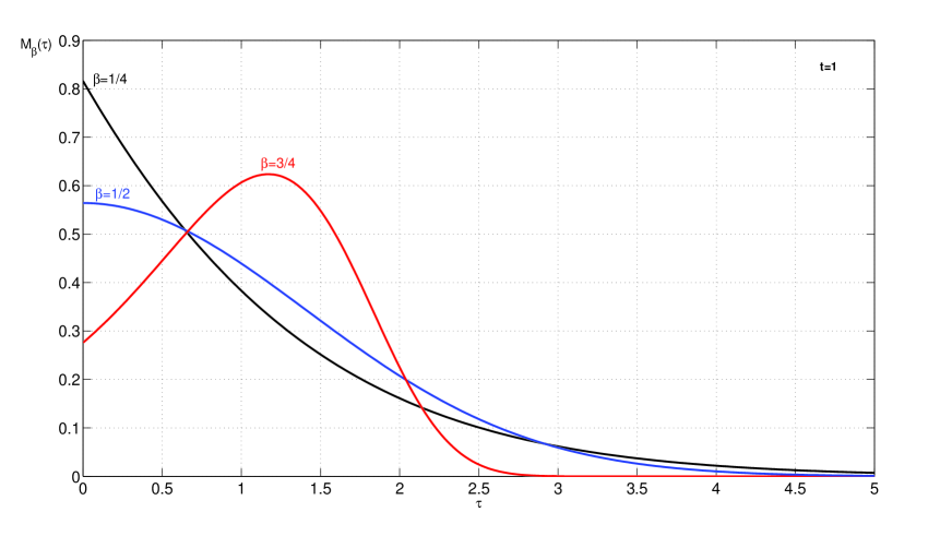
Refer to caption
Figure 1: Plot of the density function h​(Ο„,t)=tβˆ’Ξ²β€‹M​(τ​tβˆ’Ξ²)β„Žπœπ‘‘superscriptπ‘‘π›½π‘€πœsuperscript𝑑𝛽h(\tau,t)=t^{-\beta}M(\tau t^{-\beta}) at time t=1𝑑1t=1, for different values of the parameter Ξ²=[1/4,1/2,3/4]𝛽141234\beta=[1/4,1/2,3/4].
Remark 7.2.

The function h​(Ο„,t)β„Žπœπ‘‘h(\tau,t) in Eq. (59) represents the fundamental solution of the time-fractional forward drift equation (see also [15]):

u​(Ο„,t)=u0​(Ο„)βˆ’1Γ​(Ξ²)β€‹βˆ«0t(tβˆ’s)Ξ²βˆ’1β€‹βˆ‚Ο„u​(Ο„,s)​d​s.π‘’πœπ‘‘subscript𝑒0𝜏1Γ𝛽superscriptsubscript0𝑑superscript𝑑𝑠𝛽1subscriptπœπ‘’πœπ‘ π‘‘π‘ u(\tau,t)=u_{0}(\tau)-\frac{1}{\Gamma(\beta)}\int_{0}^{t}(t-s)^{\beta-1}\partial_{\tau}u(\tau,s)ds. (61)

This equation reduces to the standard drift equation when Ξ²β†’1→𝛽1\beta\rightarrow 1.

7.1.1 Properties of the M𝑀M-function

It is useful to recall some important properties of the M𝑀M-function [29, 12]. These are best expressed in terms of the function

ℳβ​(Ο„,t)=tβˆ’Ξ²β€‹Mβ​(τ​tβˆ’Ξ²),subscriptβ„³π›½πœπ‘‘superscript𝑑𝛽subscriptπ‘€π›½πœsuperscript𝑑𝛽\mathcal{M}_{\beta}(\tau,t)=t^{-\beta}M_{\beta}(\tau t^{-\beta}), (62)

defined for any Ο„,tβ‰₯0πœπ‘‘0\tau,t\geq 0 and 0<Ξ²<10𝛽10<\beta<1.

  1. 1.

    The Laplace transform of ℳβ​(Ο„,t)subscriptβ„³π›½πœπ‘‘\mathcal{M}_{\beta}(\tau,t) with respect to t𝑑t is:

    ℒ​{ℳβ​(Ο„,t);t,s}=sΞ²βˆ’1​eβˆ’Ο„β€‹sΞ²,Ο„,sβ‰₯0.formulae-sequenceβ„’subscriptβ„³π›½πœπ‘‘π‘‘π‘ superscript𝑠𝛽1superscriptπ‘’πœsuperscriptπ‘ π›½πœπ‘ 0\mathscr{L}\{\mathcal{M}_{\beta}(\tau,t);t,s\}=s^{\beta-1}e^{-\tau s^{\beta}},\;\;\tau,s\geq 0. (63)
  2. 2.

    The above equation suggests that in the singular limit Ξ²β†’1→𝛽1\beta\rightarrow 1 one has:

    β„³1​(Ο„,t)=δ​(Ο„βˆ’t),Ο„,tβ‰₯0.formulae-sequencesubscriptβ„³1πœπ‘‘π›Ώπœπ‘‘πœπ‘‘0\mathcal{M}_{1}(\tau,t)=\delta(\tau-t),\;\;\tau,t\geq 0. (64)
  3. 3.

    If Ξ²=1/2𝛽12\beta=1/2:

    β„³1/2​(Ο„,t)=1π​t​exp⁑(βˆ’Ο„2/4​t),Ο„,tβ‰₯0.formulae-sequencesubscriptβ„³12πœπ‘‘1πœ‹π‘‘superscript𝜏24π‘‘πœπ‘‘0\mathcal{M}_{1/2}(\tau,t)=\frac{1}{\sqrt{\pi t}}\exp(-\tau^{2}/4t),\;\;\tau,t\geq 0. (65)
  4. 4.

    The M𝑀M-function is a particular case of a Fox H𝐻H-function [30, 44]. We indicate with

    ℳ​{φ​(x);x,u}=∫0βˆžΟ†β€‹(x)​xuβˆ’1​𝑑x,β„³πœ‘π‘₯π‘₯𝑒superscriptsubscript0πœ‘π‘₯superscriptπ‘₯𝑒1differential-dπ‘₯\mathscr{M}\{\varphi(x);x,u\}=\int_{0}^{\infty}\varphi(x)x^{u-1}dx, (66)

    the Mellin transform of a function φ​(x)πœ‘π‘₯\varphi(x), xβ‰₯0π‘₯0x\geq 0, with respect to xπ‘₯x evaluated in uβ‰₯0𝑒0u\geq 0. The Fox H𝐻H-function

    Hp,qm,n​(z)=Hp,qm,n​(z|(ai,Ξ±i)i=1,…,p(bj,Ξ²j)j=1,…,q),subscriptsuperscriptπ»π‘šπ‘›π‘π‘žπ‘§subscriptsuperscriptπ»π‘šπ‘›π‘π‘žconditional𝑧subscriptsubscriptπ‘Žπ‘–subscript𝛼𝑖𝑖1…𝑝subscriptsubscript𝑏𝑗subscript𝛽𝑗𝑗1β€¦π‘žH^{m,n}_{p,q}(z)=H^{m,n}_{p,q}\left(z\Big{|}\begin{array}[]{l}(a_{i},\alpha_{i})_{i=1,\dots,p}\\ (b_{j},\beta_{j})_{j=1,\dots,q}\end{array}\right),

    is characterized by its Mellin transform as follows:

    ℳ​{Hp,qm,n​(z);z,u}=A​(u)​B​(u)C​(u)​D​(u),β„³subscriptsuperscriptπ»π‘šπ‘›π‘π‘žπ‘§π‘§π‘’π΄π‘’π΅π‘’πΆπ‘’π·π‘’\mathscr{M}\{H^{\;m,n}_{p,q}(z);z,u\}=\frac{A(u)B(u)}{C(u)D(u)}, (67)

    with

    A​(u)=∏i=1mΓ​(bj+Ξ²j​u),B​(u)=∏j=1nΓ​(1βˆ’ajβˆ’Ξ±j​u),C​(u)=∏i=m+1qΓ​(1βˆ’bjβˆ’Ξ²j​u),D​(u)=∏j=n+1pΓ​(aj+Ξ±j​u).𝐴𝑒superscriptsubscriptproduct𝑖1π‘šΞ“subscript𝑏𝑗subscript𝛽𝑗𝑒𝐡𝑒superscriptsubscriptproduct𝑗1𝑛Γ1subscriptπ‘Žπ‘—subscript𝛼𝑗𝑒𝐢𝑒superscriptsubscriptproductπ‘–π‘š1π‘žΞ“1subscript𝑏𝑗subscript𝛽𝑗𝑒𝐷𝑒superscriptsubscriptproduct𝑗𝑛1𝑝Γsubscriptπ‘Žπ‘—subscript𝛼𝑗𝑒\begin{array}[]{ll}A(u)=\displaystyle\prod_{i=1}^{m}\Gamma(b_{j}+\beta_{j}u),&B(u)=\displaystyle\prod_{j=1}^{n}\Gamma(1-a_{j}-\alpha_{j}u),\\ C(u)=\displaystyle\prod_{i=m+1}^{q}\Gamma(1-b_{j}-\beta_{j}u),&D(u)=\displaystyle\prod_{j=n+1}^{p}\Gamma(a_{j}+\alpha_{j}u).\end{array}

    Here: 1≀m≀q1π‘šπ‘ž1\leq m\leq q, 0≀n≀p0𝑛𝑝0\leq n\leq p, Ξ±j,Ξ²j>0subscript𝛼𝑗subscript𝛽𝑗0\alpha_{j},\beta_{j}>0 and aj,bjβˆˆβ„‚subscriptπ‘Žπ‘—subscript𝑏𝑗ℂa_{j},b_{j}\in\mathbb{C} (see [11, 33, 46] for more details).

    Starting from Eq. (63) and skipping to the Mellin transform, it is easy to show that we have the following relation:

    ℳβ​(Ο„,t)=tβˆ’Ξ²β€‹H1,11,0​(τ​tβˆ’Ξ²|(1βˆ’Ξ²,Ξ²)(0,1)),Ο„,tβ‰₯0,  0<Ξ²<1.formulae-sequencesubscriptβ„³π›½πœπ‘‘superscript𝑑𝛽subscriptsuperscript𝐻1011conditional𝜏superscript𝑑𝛽1𝛽𝛽01𝜏formulae-sequence𝑑0  0𝛽1\mathcal{M}_{\beta}(\tau,t)=t^{-\beta}H^{1,0}_{1,1}\left(\tau t^{-\beta}\Big{|}\begin{array}[]{l}(1-\beta,\beta)\\ (0,1)\end{array}\right),\;\;\tau,t\geq 0,\;\;0<\beta<1. (68)
  5. 5.

    Using the representation Eq. (68) and Eq. (67) we have for any Ξ·,β∈(0,1)πœ‚π›½01\eta,\beta\in(0,1), see also [29]:

    ℳν​(x,t)=∫0βˆžβ„³Ξ·β€‹(x,Ο„)​ℳβ​(Ο„,t)​𝑑τ,Ξ½=η​β​xβ‰₯0.formulae-sequencesubscriptβ„³πœˆπ‘₯𝑑superscriptsubscript0subscriptβ„³πœ‚π‘₯𝜏subscriptβ„³π›½πœπ‘‘differential-dπœπœˆπœ‚π›½π‘₯0\mathcal{M}_{\nu}(x,t)=\int_{0}^{\infty}\mathcal{M}_{\eta}(x,\tau)\mathcal{M}_{\beta}(\tau,t)d\tau,\;\;\nu=\eta\beta\,\;\;x\geq 0. (69)

The expression (59) for the function h​(Ο„,t)β„Žπœπ‘‘h(\tau,t) follows from Eq. (63), that is:

h​(Ο„,t)=ℳβ​(Ο„,t),Ο„,tβ‰₯0.formulae-sequenceβ„Žπœπ‘‘subscriptβ„³π›½πœπ‘‘πœπ‘‘0h(\tau,t)=\mathcal{M}_{\beta}(\tau,t),\;\;\tau,\,t\geq 0. (70)

Moreover, when Ξ²β†’1→𝛽1\beta\rightarrow 1,Eq. 64) gives h​(Ο„,t)=δ​(Ο„βˆ’t)β„Žπœπ‘‘π›Ώπœπ‘‘h(\tau,t)=\delta(\tau-t) as expected (see Remark 7.2). Comparing Eq. (9) and Eq. (65) one observes that:

G​(x,t)=12​ℳ1/2​(|x|,t).𝐺π‘₯𝑑12subscriptβ„³12π‘₯𝑑G(x,t)=\frac{1}{2}\mathcal{M}_{1/2}(|x|,t). (71)

Using Theorem 4.1 and Eq. (69) together with Eq. (70) and Eq. (71) we recover the fundamental solution of the time-fractional diffusion equation [27]:

f​(x,t)=∫0∞G​(x,Ο„)​h​(Ο„,t)​𝑑τ=12β€‹βˆ«0βˆžβ„³1/2​(|x|,Ο„)​ℳβ​(Ο„,t)​𝑑τ𝑓π‘₯𝑑superscriptsubscript0𝐺π‘₯πœβ„Žπœπ‘‘differential-d𝜏12superscriptsubscript0subscriptβ„³12π‘₯𝜏subscriptβ„³π›½πœπ‘‘differential-d𝜏f(x,t)=\int_{0}^{\infty}G(x,\tau)h(\tau,t)d\,\tau=\frac{1}{2}\int_{0}^{\infty}\mathcal{M}_{1/2}(|x|,\tau)\mathcal{M}_{\beta}(\tau,t)\,d\tau
=12​ℳβ/2​(|x|,t)=12​tβˆ’Ξ²/2​MΞ²/2​(|x|​tβˆ’Ξ²/2).absent12subscriptℳ𝛽2π‘₯𝑑12superscript𝑑𝛽2subscript𝑀𝛽2π‘₯superscript𝑑𝛽2=\frac{1}{2}\mathcal{M}_{\beta/2}(|x|,t)=\frac{1}{2}t^{-\beta/2}M_{\beta/2}(|x|t^{-\beta/2}). (72)

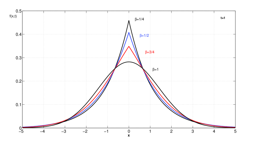
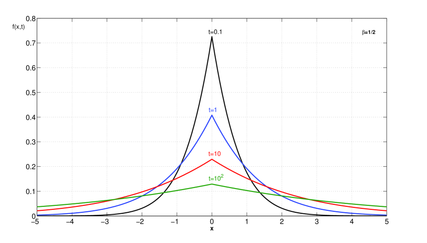
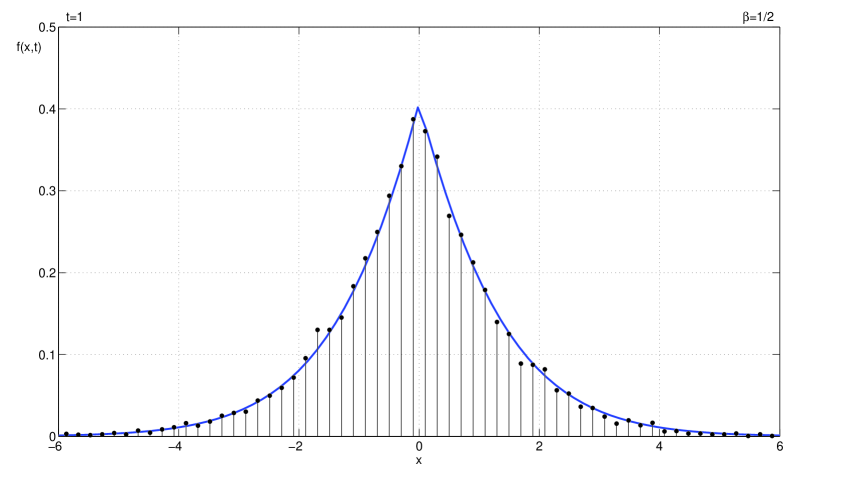
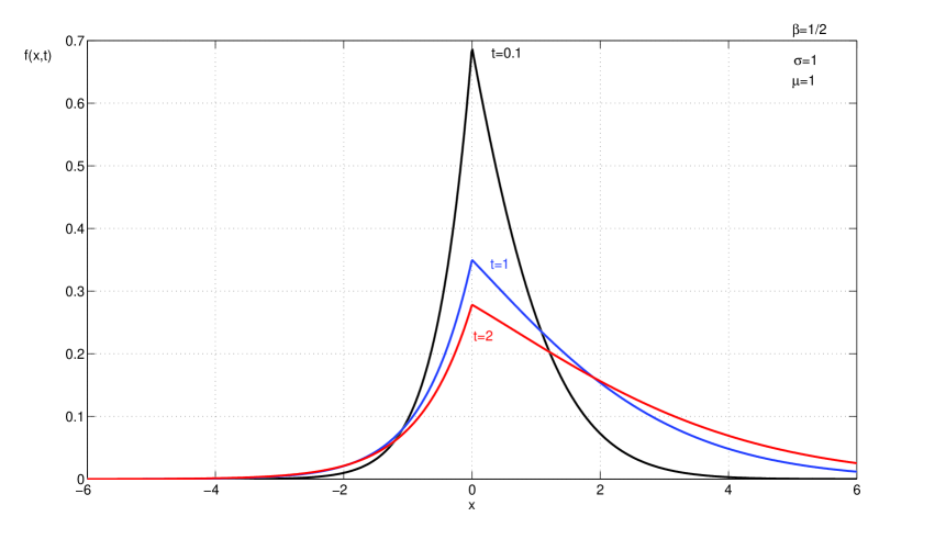
Several plots of the M𝑀M-function are presented: in Figure 1 the function h​(Ο„,t)=ℳβ​(Ο„,t)β„Žπœπ‘‘subscriptβ„³π›½πœπ‘‘h(\tau,t)=\mathcal{M}_{\beta}(\tau,t) is drawn at a fixed time t=1𝑑1t=1 and for different values of the parameter β𝛽\beta; in Figure 2 is presented the plot of f​(x,t)=12​ℳβ/2​(|x|,t)𝑓π‘₯𝑑12subscriptℳ𝛽2π‘₯𝑑f(x,t)=\frac{1}{2}\mathcal{M}_{\beta/2}(|x|,t) at a fixed time t=1𝑑1t=1 and for different values of β𝛽\beta; in Figure 3 is shown the time evolution of f​(x,t)𝑓π‘₯𝑑f(x,t) for fixed Ξ²=1/2𝛽12\beta=1/2.

Refer to caption
Figure 2: Plot of the density function f​(x,t)𝑓π‘₯𝑑f(x,t) given by Eq. (72) at time t=1𝑑1t=1, for different values of the parameter Ξ²=[1/4,1/2,3/4,1]𝛽1412341\beta=[1/4,1/2,3/4,1]. For Ξ²=1𝛽1\beta=1 one recovers the standard Gaussian density (71).
Refer to caption
Figure 3: Plot of the density function f​(x,t)𝑓π‘₯𝑑f(x,t) for fixed Ξ²=1/2𝛽12\beta=1/2, at different times t=[0.1,1,10,102]𝑑0.1110superscript102t=[0.1,1,10,10^{2}].

7.1.2 Stochastic interpretations of the solution

From a stochastic point of view, the function h​(Ο„,t)β„Žπœπ‘‘h(\tau,t) in Eq. (59) can be regarded as the marginal distribution of

lβ​(t),tβ‰₯0,subscript𝑙𝛽𝑑𝑑0l_{\beta}(t),\;\;t\geq 0,

where lβ​(t)subscript𝑙𝛽𝑑l_{\beta}(t), tβ‰₯0𝑑0t\geq 0, is an H𝐻H-ss random time with H=β𝐻𝛽H=\beta. We have that for each integer mβ‰₯0π‘š0m\geq 0:

E​(lβ​(t)m)=m!Γ​(β​m+1)​tβ​m.𝐸subscript𝑙𝛽superscriptπ‘‘π‘šπ‘šΞ“π›½π‘š1superscriptπ‘‘π›½π‘šE(l_{\beta}(t)^{m})=\frac{m!}{\Gamma(\beta m+1)}t^{\beta m}. (73)

In fact, from Eq. (58), for each integer mβ‰₯0π‘š0m\geq 0, we have :

∫0βˆžΟ„m​sΞ²βˆ’1​eβˆ’Ο„β€‹sβ​𝑑τ=m!​sβˆ’mβ€‹Ξ²βˆ’1,superscriptsubscript0superscriptπœπ‘šsuperscript𝑠𝛽1superscriptπ‘’πœsuperscript𝑠𝛽differential-dπœπ‘šsuperscriptπ‘ π‘šπ›½1\int_{0}^{\infty}\tau^{m}s^{\beta-1}e^{-\tau s^{\beta}}d\tau=m!s^{-m\beta-1},

which, inverting the Laplace transform, gives Eq. (73).

For instance, with the suitable conventions [8], lβ​(t)subscript𝑙𝛽𝑑l_{\beta}(t), tβ‰₯0,𝑑0t\geq 0, can be viewed as the local time in zero at time t𝑑t of a d=2​(1βˆ’Ξ²)𝑑21𝛽d=2(1-\beta)-dimensional Bessel process [37]. The function f​(x,t)𝑓π‘₯𝑑f(x,t) in Eq. (72) is then the marginal density function of

D​(t)=B​(lβ​(t)),𝐷𝑑𝐡subscript𝑙𝛽𝑑D(t)=B\left(l_{\beta}(t)\right),

which is self-similar with H=Ξ²/2𝐻𝛽2H=\beta/2. In this case, because lβ​(t)subscript𝑙𝛽𝑑l_{\beta}(t) is self-similar of order β𝛽\beta, we immediately have an example of a different process with the same marginal distribution of D​(t)𝐷𝑑D(t) (see Example 5.1). In fact, if we consider a β€œstandard” fractional Brownian motion BΞ²/2subscript𝐡𝛽2B_{\beta/2} of order Ξ²/2𝛽2\beta/2, then f​(x,t)𝑓π‘₯𝑑f(x,t) can also be seen as the marginal distribution of

Y​(t)=lβ​(1)​BΞ²/2​(t),π‘Œπ‘‘subscript𝑙𝛽1subscript𝐡𝛽2𝑑Y(t)=\sqrt{l_{\beta}(1)}B_{\beta/2}(t), (74)

where BΞ²/2​(t)subscript𝐡𝛽2𝑑B_{\beta/2}(t) is assumed to be independent of lβ​(1)subscript𝑙𝛽1l_{\beta}(1) (see Example 5.1). The process Y​(t)π‘Œπ‘‘Y(t), tβ‰₯0𝑑0t\geq 0, is called grey Brownian motion [43].

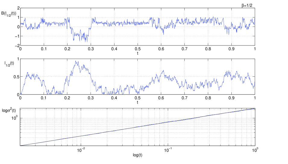
Refer to caption
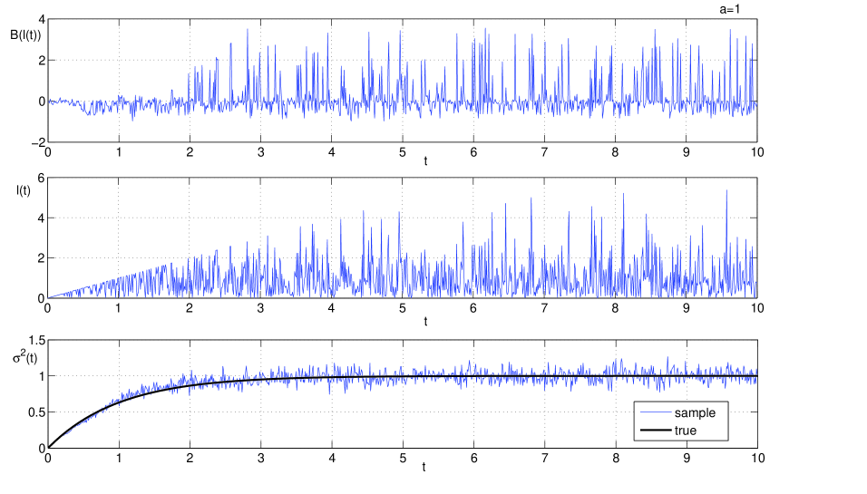
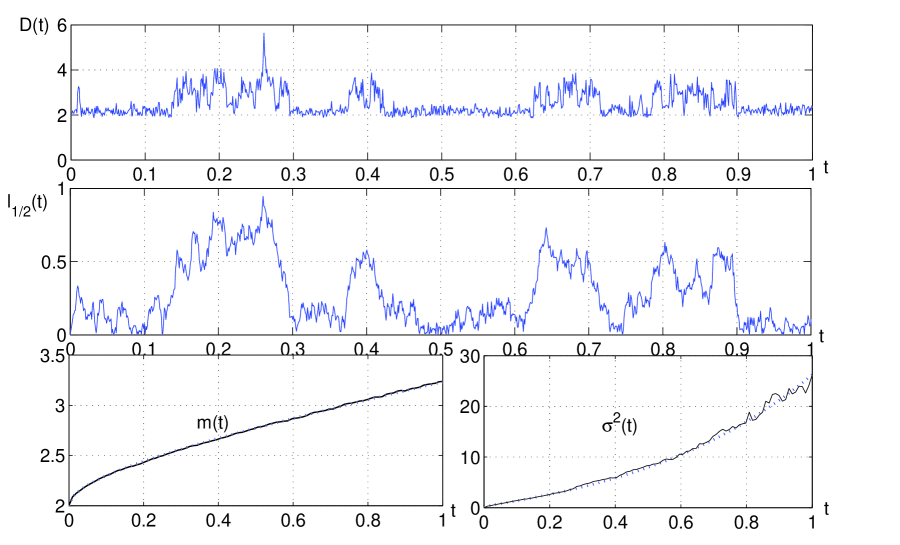
Figure 4: Trajectory of the process B​(lβ​(t))𝐡subscript𝑙𝛽𝑑B(l_{\beta}(t)) (top panel), with 0<t<10𝑑10<t<1 and Ξ²=1/2𝛽12\beta=1/2. The random time process is chosen to be l1/2​(t)=|b​(t)|subscript𝑙12𝑑𝑏𝑑l_{1/2}(t)=|b(t)| where b​(t)𝑏𝑑b(t) is a β€œstandard” Brownian motion (see Example 1.1). The corresponding trajectory of the random time process is presented in the middle panel. The estimated variance, computed on a sample of dimension N=5000𝑁5000N=5000, is presented in logarithmic scale in the bottom panel and fits perfectly the theoretical curve 2​t1/2/Γ​(3/2)2superscript𝑑12Ξ“322t^{1/2}/\Gamma(3/2).

From Eq. (73) one can derive immediately all the moments for the processes D​(t)𝐷𝑑D(t) and Y​(t)π‘Œπ‘‘Y(t). For any integer mβ‰₯0π‘š0m\geq 0

{E​(D​(t)2​m+1)=E​(Y​(t)2​m+1)=0;E​(D​(t)2​m)=E​(Y​(t)2​m)=2​m!Γ​(β​m+1)​tβ​m.cases𝐸𝐷superscript𝑑2π‘š1πΈπ‘Œsuperscript𝑑2π‘š10missing-subexpression𝐸𝐷superscript𝑑2π‘šπΈπ‘Œsuperscript𝑑2π‘š2π‘šΞ“π›½π‘š1superscriptπ‘‘π›½π‘šmissing-subexpression\left\{\begin{array}[]{ll}E(D(t)^{2m+1})=E(Y(t)^{2m+1})=0;\\[8.5359pt] E(D(t)^{2m})=E(Y(t)^{2m})=\displaystyle\frac{2m!}{\Gamma(\beta m+1)}t^{\beta m}.\end{array}\right. (75)

Because 0<Ξ²<10𝛽10<\beta<1, the variance grows slower than linearly with respect to time. In this case one speaks about slow anomalous diffusion. Moreover, the increments of the fractional Brownian motion BΞ²/2​(t)subscript𝐡𝛽2𝑑B_{\beta/2}(t) do not have long-range dependence. In contrast, the next example allows for the presence of long-range dependence through the introduction of a scaling function g​(t)=tΞ±/β𝑔𝑑superscript𝑑𝛼𝛽g(t)=t^{\alpha/\beta} (see also Example 1.2).

Refer to caption
Figure 5: Marginal density function f​(x,t)=12​ℳ1/4​(|x|,t)𝑓π‘₯𝑑12subscriptβ„³14π‘₯𝑑f(x,t)=\frac{1}{2}\mathcal{M}_{1/4}(|x|,t) of the process B​(l1/2​(t))𝐡subscript𝑙12𝑑B(l_{1/2}(t)) at time t=1𝑑1t=1 and x∈[βˆ’5,5]π‘₯55x\in[-5,5]. The histogram is evaluated over N=104𝑁superscript104N=10^{4} simulated trajectories of the process B​(|b​(t)|)𝐡𝑏𝑑B(|b(t)|) (Figure 4).

7.2 β€œStretched” time-fractional diffusion equation

If in the setup of Section 7.1, where the kernel K​(t)𝐾𝑑K(t) is given by Eq. (56), we introduce a scaling time

g​(t)=tΞ±/β𝑔𝑑superscript𝑑𝛼𝛽g(t)=t^{\alpha/\beta}

with Ξ±>0𝛼0\alpha>0, then the integral equation (57) is replaced by Eq. (37), namely

u​(x,t)=u0​(t)+1Γ​(Ξ²)β€‹Ξ±Ξ²β€‹βˆ«0tsΞ±Ξ²βˆ’1​(tΞ±Ξ²βˆ’sΞ±Ξ²)Ξ²βˆ’1β€‹βˆ‚x​xu​(x,s)​d​s.𝑒π‘₯𝑑subscript𝑒0𝑑1Γ𝛽𝛼𝛽superscriptsubscript0𝑑superscript𝑠𝛼𝛽1superscriptsuperscript𝑑𝛼𝛽superscript𝑠𝛼𝛽𝛽1subscriptπ‘₯π‘₯𝑒π‘₯𝑠𝑑𝑠u(x,t)=u_{0}(t)+\frac{1}{\Gamma(\beta)}\frac{\alpha}{\beta}\int_{0}^{t}s^{\frac{\alpha}{\beta}-1}\left(t^{\frac{\alpha}{\beta}}-s^{\frac{\alpha}{\beta}}\right)^{\beta-1}\partial_{xx}u(x,s)ds. (76)

Therefore, using Eq. 59):

h​(Ο„,g​(t))=g​(t)βˆ’Ξ²β€‹Mβ​(τ​g​(t)βˆ’Ξ²)=tβˆ’Ξ±β€‹Mβ​(τ​tβˆ’Ξ±),β„Žπœπ‘”π‘‘π‘”superscript𝑑𝛽subscriptπ‘€π›½πœπ‘”superscript𝑑𝛽superscript𝑑𝛼subscriptπ‘€π›½πœsuperscript𝑑𝛼h(\tau,g(t))=g(t)^{-\beta}M_{\beta}(\tau g(t)^{-\beta})=t^{-\alpha}M_{\beta}(\tau t^{-\alpha}),

and, using Eq. (72), the fundamental solution f¯​(x,t)¯𝑓π‘₯𝑑\overline{f}(x,t) of Eq. (76) reads:

f¯​(x,t)=f​(x,g​(t))=12​tβˆ’Ξ±/2​MΞ²/2​(|x|​tβˆ’Ξ±/2),tβ‰₯0.formulae-sequence¯𝑓π‘₯𝑑𝑓π‘₯𝑔𝑑12superscript𝑑𝛼2subscript𝑀𝛽2π‘₯superscript𝑑𝛼2𝑑0\overline{f}(x,t)=f(x,g(t))=\frac{1}{2}t^{-\alpha/2}M_{\beta/2}(|x|t^{-\alpha/2}),\;\;t\geq 0. (77)

The function f¯​(x,t)¯𝑓π‘₯𝑑\overline{f}(x,t), tβ‰₯0𝑑0t\geq 0, is the marginal distribution of the process

D(t)=B(lΞ²(tΞ±/Ξ²))),tβ‰₯0.D(t)=B\left(l_{\beta}(t^{\alpha/\beta}))\right),\;\;t\geq 0.

The time-change process lβ​(tΞ±/Ξ²)subscript𝑙𝛽superscript𝑑𝛼𝛽l_{\beta}(t^{\alpha/\beta}) is self-similar of order H=α𝐻𝛼H=\alpha and the process D​(t)𝐷𝑑D(t) is then self-similar with H=Ξ±/2𝐻𝛼2H=\alpha/2. In the case 0<Ξ±<20𝛼20<\alpha<2, the function f¯​(x,t)¯𝑓π‘₯𝑑\overline{f}(x,t) is also the marginal density of

𝒴​(t)=lβ​(1)​BΞ±/2​(t),tβ‰₯0,  0<Ξ±<2,formulae-sequence𝒴𝑑subscript𝑙𝛽1subscript𝐡𝛼2𝑑formulae-sequence𝑑0  0𝛼2\mathcal{Y}(t)=\sqrt{l_{\beta}(1)}B_{\alpha/2}(t),\;\;t\geq 0,\;\;0<\alpha<2, (78)

where BΞ±/2​(t)subscript𝐡𝛼2𝑑B_{\alpha/2}(t) is a β€œstandard” fBm of order H=Ξ±/2𝐻𝛼2H=\alpha/2 independent of lβ​(1)subscript𝑙𝛽1l_{\beta}(1). The process 𝒴​(t)𝒴𝑑\mathcal{Y}(t), tβ‰₯0𝑑0t\geq 0, is called generalized grey Brownian motion [38].

In this case, for any integer mβ‰₯0π‘š0m\geq 0:

{E​(D​(t)2​m+1)=E​(𝒴​(t)2​m+1)=0;E​(D​(t)2​m)=E​(𝒴​(t)2​m)=2​m!Γ​(β​m+1)​tα​m.cases𝐸𝐷superscript𝑑2π‘š1𝐸𝒴superscript𝑑2π‘š10missing-subexpression𝐸𝐷superscript𝑑2π‘šπΈπ’΄superscript𝑑2π‘š2π‘šΞ“π›½π‘š1superscriptπ‘‘π›Όπ‘šmissing-subexpression\left\{\begin{array}[]{ll}E(D(t)^{2m+1})=E(\mathcal{Y}(t)^{2m+1})=0;\\[8.5359pt] E(D(t)^{2m})=E(\mathcal{Y}(t)^{2m})=\displaystyle\frac{2m!}{\Gamma(\beta m+1)}t^{\alpha m}.\end{array}\right. (79)

We have slow diffusion when 0<Ξ±<10𝛼10<\alpha<1 (the variance grows slower than linearly in time) and fast diffusion when 1<Ξ±<21𝛼21<\alpha<2 (the variance grows faster than linearly in time). In this case the increments of the process 𝒴​(t)𝒴𝑑\mathcal{Y}(t) exhibit long-range dependence.

Refer to caption
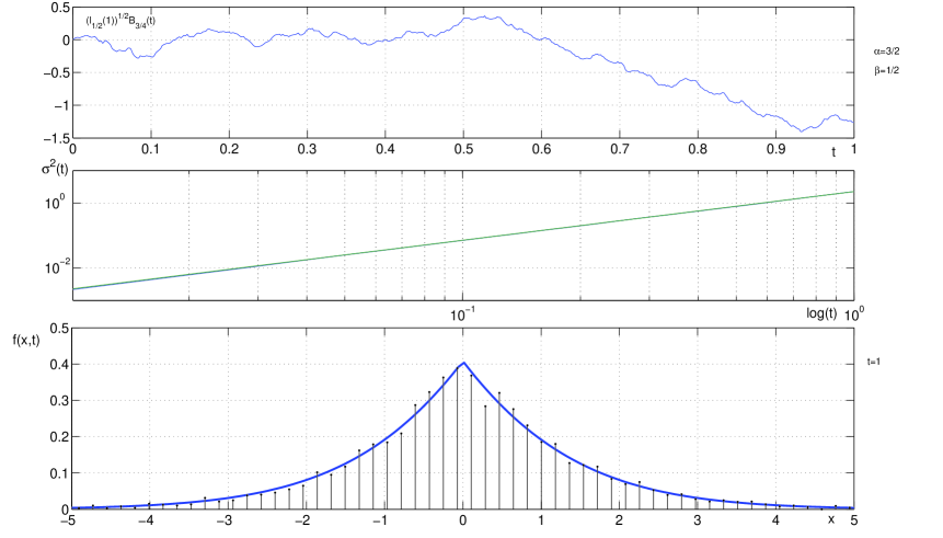
Figure 6: Trajectory of the process lβ​(1)​BΞ±/2​(t)subscript𝑙𝛽1subscript𝐡𝛼2𝑑\sqrt{l_{\beta}(1)}B_{\alpha/2}(t) (top panel), with 0<t<10𝑑10<t<1, Ξ²=1/2𝛽12\beta=1/2 and Ξ±=3/2𝛼32\alpha=3/2. The random variable l1/2​(1)subscript𝑙121l_{1/2}(1) is Gaussian, see Eq. (65). The estimated variance, computed on a sample of dimension N=5000𝑁5000N=5000, is presented in logarithmic scale in the middle panel together with the theoretical curve 2​t3/2/Γ​(3/2)2superscript𝑑32Ξ“322t^{3/2}/\Gamma(3/2). In the bottom panel the histogram, evaluated over a sample of N=104𝑁superscript104N=10^{4} trajectories, fits the exact marginal density Eq. (77) at time t=1𝑑1t=1.

7.3 Exponential-decay kernel

Let g​(t)=t𝑔𝑑𝑑g(t)=t. With the exponential-decay kernel:

K​(t)=exp⁑(βˆ’a​t),aβ‰₯0,tβ‰₯0,formulae-sequenceπΎπ‘‘π‘Žπ‘‘formulae-sequenceπ‘Ž0𝑑0K(t)=\exp(-at),\;\;a\geq 0,\;\;t\geq 0, (80)

we obtain the following equation:

u​(x,t)=u0​(x)+∫0teβˆ’a​(tβˆ’s)β€‹βˆ‚x​xu​(x,s)​d​s.𝑒π‘₯𝑑subscript𝑒0π‘₯superscriptsubscript0𝑑superscriptπ‘’π‘Žπ‘‘π‘ subscriptπ‘₯π‘₯𝑒π‘₯𝑠𝑑𝑠u(x,t)=u_{0}(x)+\int_{0}^{t}e^{-a(t-s)}\partial_{xx}u(x,s)ds. (81)

In this case K~​(s)=(s+a)βˆ’1~𝐾𝑠superscriptπ‘ π‘Ž1\widetilde{K}(s)=(s+a)^{-1} and the marginal distribution of the random time process l​(t)𝑙𝑑l(t), tβ‰₯0𝑑0t\geq 0, is defined by Eq. (26):

ℒ​{fl​(Ο„,t);t,s}=s+as​eβˆ’Ο„β€‹(s+a),Ο„β‰₯0.formulae-sequenceβ„’subscriptπ‘“π‘™πœπ‘‘π‘‘π‘ π‘ π‘Žπ‘ superscriptπ‘’πœπ‘ π‘Žπœ0\mathscr{L}\{f_{l}(\tau,t);t,s\}=\frac{s+a}{s}e^{-\tau(s+a)},\;\;\tau\geq 0.

Therefore,

fl​(Ο„,t)=eβˆ’Ο„β€‹a​(δ​(Ο„βˆ’t)+a​θ​(tβˆ’Ο„))=eβˆ’t​a​δ​(Ο„βˆ’t)+a​eβˆ’Ο„β€‹a​θ​(tβˆ’Ο„),subscriptπ‘“π‘™πœπ‘‘superscriptπ‘’πœπ‘Žπ›Ώπœπ‘‘π‘Žπœƒπ‘‘πœsuperscriptπ‘’π‘‘π‘Žπ›Ώπœπ‘‘π‘Žsuperscriptπ‘’πœπ‘Žπœƒπ‘‘πœf_{l}(\tau,t)=e^{-\tau a}\left(\delta(\tau-t)+a\theta(t-\tau)\right)=e^{-ta}\delta(\tau-t)+ae^{-\tau a}\theta(t-\tau), (82)

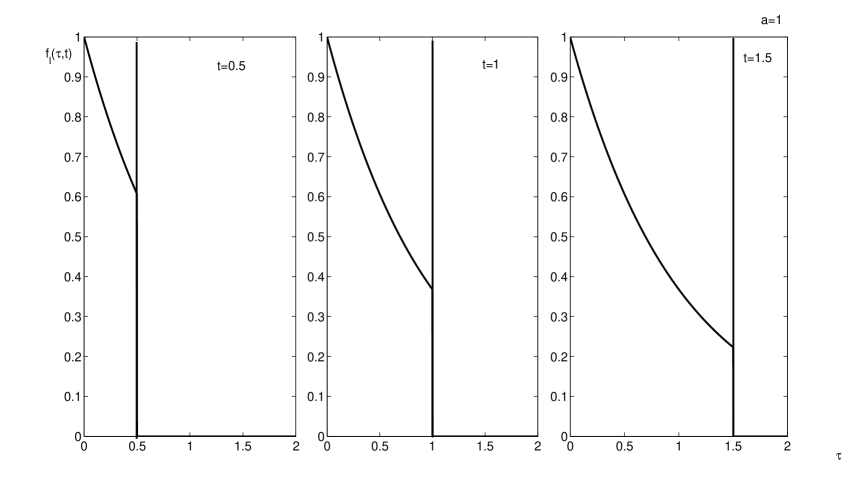
where θ​(x)πœƒπ‘₯\theta(x) is the step function (28). A graphical representation of the time evolution of fl​(Ο„,t)subscriptπ‘“π‘™πœπ‘‘f_{l}(\tau,t) is presented in Figure 7.

Refer to caption
Figure 7: Plots of the marginal density of the random time fl​(Ο„,t)subscriptπ‘“π‘™πœπ‘‘f_{l}(\tau,t)Eq. 82) as a function of Ο„πœ\tau at times t=[0.5,1,1.5]𝑑0.511.5t=[0.5,1,1.5], and with a=1π‘Ž1a=1. The vertical line corresponds to a point mass (delta function).
Remark 7.3.

The function fl​(Ο„,t)subscriptπ‘“π‘™πœπ‘‘f_{l}(\tau,t) defined in Eq. 82) is the fundamental solution, in the sense of distributions, of the β€œexponential” forward drift equation:

u​(Ο„,t)=u0​(Ο„)βˆ’βˆ«0teβˆ’a​(tβˆ’s)β€‹βˆ‚Ο„u​(Ο„,s)​d​s.π‘’πœπ‘‘subscript𝑒0𝜏superscriptsubscript0𝑑superscriptπ‘’π‘Žπ‘‘π‘ subscriptπœπ‘’πœπ‘ π‘‘π‘ u(\tau,t)=u_{0}(\tau)-\int_{0}^{t}e^{-a(t-s)}\partial_{\tau}u(\tau,s)ds.

This follows from Proposition 3.1. To check it directly we note that fl​(Ο„,0)=δ​(Ο„)subscriptπ‘“π‘™πœ0π›Ώπœf_{l}(\tau,0)=\delta(\tau) and for any t>0𝑑0t>0:

βˆ’βˆ«0teβˆ’a​(tβˆ’s)β€‹βˆ‚Ο„fl​(Ο„,s)​d​s=βˆ’βˆ«0teβˆ’a​(tβˆ’s)β€‹βˆ‚Ο„(eβˆ’a​s​δ​(Ο„βˆ’s)+a​eβˆ’a​τ​θ​(sβˆ’Ο„))​d​ssuperscriptsubscript0𝑑superscriptπ‘’π‘Žπ‘‘π‘ subscript𝜏subscriptπ‘“π‘™πœπ‘ π‘‘π‘ superscriptsubscript0𝑑superscriptπ‘’π‘Žπ‘‘π‘ subscript𝜏superscriptπ‘’π‘Žπ‘ π›Ώπœπ‘ π‘Žsuperscriptπ‘’π‘Žπœπœƒπ‘ πœπ‘‘π‘ -\int_{0}^{t}e^{-a(t-s)}\partial_{\tau}f_{l}(\tau,s)ds=-\int_{0}^{t}e^{-a(t-s)}\partial_{\tau}\left(e^{-as}\delta(\tau-s)+ae^{-a\tau}\theta(s-\tau)\right)ds
=βˆ’βˆ«0teβˆ’a​(tβˆ’s)​(βˆ’eβˆ’a​s​δ′​(Ο„βˆ’s)+a​eβˆ’a​τ​δ​(sβˆ’Ο„)βˆ’a2​eβˆ’a​τ​θ​(sβˆ’Ο„))​𝑑sabsentsuperscriptsubscript0𝑑superscriptπ‘’π‘Žπ‘‘π‘ superscriptπ‘’π‘Žπ‘ superscriptπ›Ώβ€²πœπ‘ π‘Žsuperscriptπ‘’π‘Žπœπ›Ώπ‘ πœsuperscriptπ‘Ž2superscriptπ‘’π‘Žπœπœƒπ‘ πœdifferential-d𝑠=-\int_{0}^{t}e^{-a(t-s)}\left(-e^{-as}\delta^{\prime}(\tau-s)+ae^{-a\tau}\delta(s-\tau)-a^{2}e^{-a\tau}\theta(s-\tau)\right)\,ds
=eβˆ’a​t​δ​(Ο„βˆ’t)+a​eβˆ’a​t​θ​(tβˆ’Ο„)+a​eβˆ’a​(t+Ο„)​θ​(tβˆ’Ο„)​(ea​tβˆ’ea​τ)absentsuperscriptπ‘’π‘Žπ‘‘π›Ώπœπ‘‘π‘Žsuperscriptπ‘’π‘Žπ‘‘πœƒπ‘‘πœπ‘Žsuperscriptπ‘’π‘Žπ‘‘πœπœƒπ‘‘πœsuperscriptπ‘’π‘Žπ‘‘superscriptπ‘’π‘Žπœ=e^{-at}\delta(\tau-t)+ae^{-at}\theta(t-\tau)+ae^{-a(t+\tau)}\theta(t-\tau)(e^{at}-e^{a\tau})
=eβˆ’a​t​δ​(Ο„βˆ’t)+a​eβˆ’a​τ​θ​(tβˆ’Ο„)=fl​(Ο„,t),absentsuperscriptπ‘’π‘Žπ‘‘π›Ώπœπ‘‘π‘Žsuperscriptπ‘’π‘Žπœπœƒπ‘‘πœsubscriptπ‘“π‘™πœπ‘‘=e^{-at}\delta(\tau-t)+ae^{-a\tau}\theta(t-\tau)=f_{l}(\tau,t),

where we have used the fact that:

∫0tδ′​(Ο„βˆ’s)​𝑑s=δ​(tβˆ’Ο„).superscriptsubscript0𝑑superscriptπ›Ώβ€²πœπ‘ differential-dπ‘ π›Ώπ‘‘πœ\int_{0}^{t}\delta^{\prime}(\tau-s)ds=\delta(t-\tau).

We observe that when aβ†’0β†’π‘Ž0a\rightarrow 0 we recover the forward drift equation (5) and indeed fl​(Ο„,t)=δ​(Ο„βˆ’t)subscriptπ‘“π‘™πœπ‘‘π›Ώπœπ‘‘f_{l}(\tau,t)=\delta(\tau-t).

As noted in Example 3.2, Eq. (82) actually defines a probability density for any tβ‰₯0𝑑0t\geq 0. The following proposition provides its moments.

Proposition 7.1.

For each integer mβ‰₯0π‘š0m\geq 0 one has:

E​(l​(t)m)=m!am​(1βˆ’eβˆ’a​t)+eβˆ’a​t​(tmβˆ’βˆ‘k=1mm!k!​tk​akβˆ’m).𝐸𝑙superscriptπ‘‘π‘šπ‘šsuperscriptπ‘Žπ‘š1superscriptπ‘’π‘Žπ‘‘superscriptπ‘’π‘Žπ‘‘superscriptπ‘‘π‘šsuperscriptsubscriptπ‘˜1π‘šπ‘šπ‘˜superscriptπ‘‘π‘˜superscriptπ‘Žπ‘˜π‘šE(l(t)^{m})=\frac{m!}{a^{m}}\left(1-e^{-at}\right)+e^{-at}\left(t^{m}-\sum_{k=1}^{m}\frac{m!}{k!}t^{k}a^{k-m}\right). (83)

Proof: for any tβ‰₯0𝑑0t\geq 0, we must evaluate:

∫0βˆžΟ„m​fl​(Ο„,t)​𝑑τ=eβˆ’a​t​tm+aβ€‹βˆ«0tΟ„m​eβˆ’a​τ​𝑑τ,superscriptsubscript0superscriptπœπ‘šsubscriptπ‘“π‘™πœπ‘‘differential-d𝜏superscriptπ‘’π‘Žπ‘‘superscriptπ‘‘π‘šπ‘Žsuperscriptsubscript0𝑑superscriptπœπ‘šsuperscriptπ‘’π‘Žπœdifferential-d𝜏\int_{0}^{\infty}\tau^{m}f_{l}(\tau,t)d\tau=e^{-at}t^{m}+a\int_{0}^{t}\tau^{m}e^{-a\tau}d\tau,

where we have used Eq. (82). In order to evaluate the exponential integral in the above equation we write:

aβ€‹βˆ«0tΟ„m​eβˆ’a​τ​𝑑τ=(βˆ’1)m​aβ€‹βˆ‚am[(1βˆ’eβˆ’a​t)​(aβˆ’1)]=(βˆ’1)m​aβ€‹βˆ‘k=0m(mk)β€‹βˆ‚ak(1βˆ’eβˆ’a​t)β€‹βˆ‚amβˆ’k(aβˆ’1)π‘Žsuperscriptsubscript0𝑑superscriptπœπ‘šsuperscriptπ‘’π‘Žπœdifferential-d𝜏superscript1π‘šπ‘Žsubscriptsuperscriptπ‘šπ‘Ždelimited-[]1superscriptπ‘’π‘Žπ‘‘superscriptπ‘Ž1superscript1π‘šπ‘Žsuperscriptsubscriptπ‘˜0π‘šπ‘šmissing-subexpressionπ‘˜missing-subexpressionsubscriptsuperscriptπ‘˜π‘Ž1superscriptπ‘’π‘Žπ‘‘subscriptsuperscriptπ‘šπ‘˜π‘Žsuperscriptπ‘Ž1a\int_{0}^{t}\tau^{m}e^{-a\tau}d\tau=(-1)^{m}a\partial^{m}_{a}\left[(1-e^{-at})(a^{-1})\right]=(-1)^{m}a\sum_{k=0}^{m}\left(\!\!\begin{array}[]{cc}m\\ k\end{array}\!\!\right)\partial^{k}_{a}(1-e^{-at})\partial^{m-k}_{a}(a^{-1})
=βˆ‘k=0m(βˆ’1)k​m!k!​akβˆ’mβ€‹βˆ‚ak(1βˆ’eβˆ’a​t)=m!am​(1βˆ’eβˆ’a​t)βˆ’βˆ‘k=1mm!k!​tk​akβˆ’m​eβˆ’a​tabsentsuperscriptsubscriptπ‘˜0π‘šsuperscript1π‘˜π‘šπ‘˜superscriptπ‘Žπ‘˜π‘šsubscriptsuperscriptπ‘˜π‘Ž1superscriptπ‘’π‘Žπ‘‘π‘šsuperscriptπ‘Žπ‘š1superscriptπ‘’π‘Žπ‘‘superscriptsubscriptπ‘˜1π‘šπ‘šπ‘˜superscriptπ‘‘π‘˜superscriptπ‘Žπ‘˜π‘šsuperscriptπ‘’π‘Žπ‘‘=\sum_{k=0}^{m}(-1)^{k}\frac{m!}{k!}a^{k-m}\partial^{k}_{a}(1-e^{-at})=\frac{m!}{a^{m}}(1-e^{-at})-\sum_{k=1}^{m}\frac{m!}{k!}t^{k}a^{k-m}e^{-at}

thus one has Eq. 83). β–‘β–‘\Box

The function fl​(Ο„,t)subscriptπ‘“π‘™πœπ‘‘f_{l}(\tau,t) can be written:

fl​(Ο„,t)=eβˆ’a​t​δ​(Ο„βˆ’t)+(1βˆ’eβˆ’a​t)​φ​(Ο„,t),Ο„,tβ‰₯0,aβ‰₯0,formulae-sequencesubscriptπ‘“π‘™πœπ‘‘superscriptπ‘’π‘Žπ‘‘π›Ώπœπ‘‘1superscriptπ‘’π‘Žπ‘‘πœ‘πœπ‘‘πœformulae-sequence𝑑0π‘Ž0f_{l}(\tau,t)=e^{-at}\delta(\tau-t)+(1-e^{-at})\varphi(\tau,t),\;\;\tau,t\geq 0,\;\;a\geq 0, (84)

where:

φ​(Ο„,t)=a​eβˆ’a​τ​θ​(tβˆ’Ο„)1βˆ’eβˆ’a​t,Ο„,tβ‰₯0,aβ‰₯0.formulae-sequenceπœ‘πœπ‘‘π‘Žsuperscriptπ‘’π‘Žπœπœƒπ‘‘πœ1superscriptπ‘’π‘Žπ‘‘πœformulae-sequence𝑑0π‘Ž0\varphi(\tau,t)=a\frac{e^{-a\tau}\theta(t-\tau)}{1-e^{-at}},\;\;\tau,t\geq 0,\;\;a\geq 0. (85)

Because fl​(Ο„,t)subscriptπ‘“π‘™πœπ‘‘f_{l}(\tau,t) is a probability density, then so is φ​(Ο„,t)πœ‘πœπ‘‘\varphi(\tau,t). The corresponding random time process l​(t)𝑙𝑑l(t), tβ‰₯0𝑑0t\geq 0, can then be chosen to be:

l​(t)=bt​t+(1βˆ’bt)​j​(t),tβ‰₯0,formulae-sequence𝑙𝑑subscript𝑏𝑑𝑑1subscript𝑏𝑑𝑗𝑑𝑑0l(t)=b_{t}t+(1-b_{t})j(t),\;\;t\geq 0, (86)

where btsubscript𝑏𝑑b_{t}, tβ‰₯0𝑑0t\geq 0, is a stochastic process such that, for any fixed tβ‰₯0𝑑0t\geq 0, btsubscript𝑏𝑑b_{t} is a Bernoulli random variable with P​r​(bt=1)=eβˆ’a​tπ‘ƒπ‘Ÿsubscript𝑏𝑑1superscriptπ‘’π‘Žπ‘‘Pr(b_{t}=1)=e^{-at} and P​r​(bt=0)=1βˆ’eβˆ’a​tπ‘ƒπ‘Ÿsubscript𝑏𝑑01superscriptπ‘’π‘Žπ‘‘Pr(b_{t}=0)=1-e^{-at}, and j​(t)𝑗𝑑j(t), tβ‰₯0𝑑0t\geq 0, is a stochastic process, independent of btsubscript𝑏𝑑b_{t}, with marginal distribution given by φ​(Ο„,t)πœ‘πœπ‘‘\varphi(\tau,t).

Remark 7.4.

The random time l​(t)𝑙𝑑l(t) defined by Eq. (86) cannot be increasing everywhere. This is due to the fact that btsubscript𝑏𝑑b_{t} and j​(t)𝑗𝑑j(t) are independent and P​r​(j​(t)<t)=1π‘ƒπ‘Ÿπ‘—π‘‘π‘‘1Pr(j(t)<t)=1 for any tβ‰₯0𝑑0t\geq 0. Indeed, suppose that l​(t)𝑙𝑑l(t) is increasing. This implies that for any tβ‰₯0𝑑0t\geq 0 and Ο΅>0italic-Ο΅0\epsilon>0:

1=P​r​(l​(t+Ο΅)β‰₯l​(t)|bt=1)=P​r​(l​(t+Ο΅)β‰₯t)1π‘ƒπ‘Ÿπ‘™π‘‘italic-Ο΅conditional𝑙𝑑subscript𝑏𝑑1π‘ƒπ‘Ÿπ‘™π‘‘italic-ϡ𝑑1=Pr(l(t+\epsilon)\geq l(t)\big{|}\,b_{t}=1)=Pr(l(t+\epsilon)\geq t)
=P​r​(l​(t+Ο΅)β‰₯t|bt+Ο΅=1)​P​r​(bt+Ο΅=1)+P​r​(l​(t+Ο΅)β‰₯t|bt+Ο΅=0)​P​r​(bt+Ο΅=0)absentπ‘ƒπ‘Ÿπ‘™π‘‘italic-Ο΅conditional𝑑subscript𝑏𝑑italic-Ο΅1π‘ƒπ‘Ÿsubscript𝑏𝑑italic-Ο΅1π‘ƒπ‘Ÿπ‘™π‘‘italic-Ο΅conditional𝑑subscript𝑏𝑑italic-Ο΅0π‘ƒπ‘Ÿsubscript𝑏𝑑italic-Ο΅0=Pr(l(t+\epsilon)\geq t\big{|}\,b_{t+\epsilon}=1)Pr(b_{t+\epsilon}=1)+Pr(l(t+\epsilon)\geq t\big{|}\,b_{t+\epsilon}=0)Pr(b_{t+\epsilon}=0)
=eβˆ’a​(t+Ο΅)+(1βˆ’eβˆ’a​(t+Ο΅))​P​r​(j​(t+Ο΅)β‰₯t)absentsuperscriptπ‘’π‘Žπ‘‘italic-Ο΅1superscriptπ‘’π‘Žπ‘‘italic-Ο΅π‘ƒπ‘Ÿπ‘—π‘‘italic-ϡ𝑑=e^{-a(t+\epsilon)}+\left(1-e^{-a(t+\epsilon)}\right)Pr(j(t+\epsilon)\geq t)
=1βˆ’(1βˆ’eβˆ’a​(t+Ο΅))​P​r​(j​(t+Ο΅)<t)absent11superscriptπ‘’π‘Žπ‘‘italic-Ο΅π‘ƒπ‘Ÿπ‘—π‘‘italic-ϡ𝑑=1-\left(1-e^{-a(t+\epsilon)}\right)Pr(j(t+\epsilon)<t)

therefore taking Ο΅β†’0β†’italic-Ο΅0\epsilon\rightarrow 0 we get 1=eβˆ’a​t1superscriptπ‘’π‘Žπ‘‘1=e^{-at} with a,tβ‰₯0π‘Žπ‘‘0a,t\geq 0, which is a contradiction as soon as aβ‰ 0π‘Ž0a\neq 0 and t>0𝑑0t>0.

On the other hand, a trivial example of an increasing process with marginal distribution given by Eq. (82) is:

l¯​(t)=min⁑(X,t),tβ‰₯0,formulae-sequence¯𝑙𝑑𝑋𝑑𝑑0\overline{l}(t)=\min(X,t),\;\;t\geq 0, (87)

where X𝑋X is an exponentially distributed random variable: X∼a​eβˆ’a​τsimilar-toπ‘‹π‘Žsuperscriptπ‘’π‘ŽπœX\sim ae^{-a\tau}, Ο„β‰₯0𝜏0\tau\geq 0.

We now turn to Eq. 81). We have the following result:

Proposition 7.2.
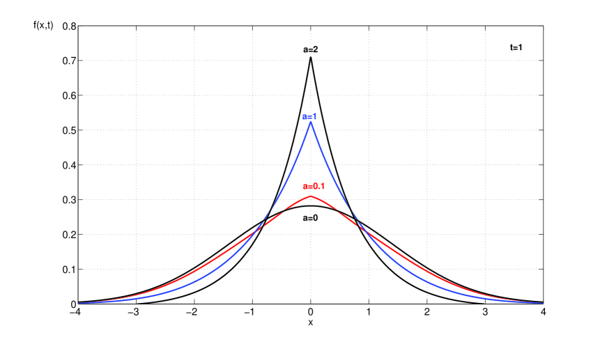
The fundamental solution of Eq. (81) is:

f​(x,t)=eβˆ’a​t​G​(x,t)+(1βˆ’eβˆ’a​t)​ϕ​(x,t),𝑓π‘₯𝑑superscriptπ‘’π‘Žπ‘‘πΊπ‘₯𝑑1superscriptπ‘’π‘Žπ‘‘italic-Ο•π‘₯𝑑f(x,t)=e^{-at}G(x,t)+(1-e^{-at})\phi(x,t), (88)

with:

ϕ​(x,t)=a4​(1βˆ’eβˆ’a​t)​{ex​a​Erf​(x2​t+a​t)βˆ’eβˆ’x​a​Erf​(x2​tβˆ’a​t)βˆ’2​sinh⁑(|x|​a)},italic-Ο•π‘₯π‘‘π‘Ž41superscriptπ‘’π‘Žπ‘‘superscript𝑒π‘₯π‘ŽErfπ‘₯2π‘‘π‘Žπ‘‘superscript𝑒π‘₯π‘ŽErfπ‘₯2π‘‘π‘Žπ‘‘2π‘₯π‘Ž\phi(x,t)=\frac{\sqrt{a}}{4(1-e^{-at})}\left\{e^{x\sqrt{a}}\textrm{\rm Erf}\left(\frac{x}{2\sqrt{t}}+\sqrt{at}\right)-e^{-x\sqrt{a}}\textrm{\rm Erf}\left(\frac{x}{2\sqrt{t}}-\sqrt{at}\right)-2\sinh(|x|\sqrt{a})\right\}, (89)

where Erf(x)=2Ο€β€‹βˆ«0xeβˆ’y2​𝑑yπ‘₯2πœ‹superscriptsubscript0π‘₯superscript𝑒superscript𝑦2differential-d𝑦(x)=\frac{2}{\sqrt{\pi}}\int_{0}^{x}e^{-y^{2}}dy and where Erf(βˆ’x)=βˆ’π‘₯(-x)=-Erf(x)π‘₯(x).

Refer to caption
Figure 8: Plot of the fundamental solution f​(x,t)𝑓π‘₯𝑑f(x,t), Eq. (88), at time t=1𝑑1t=1, for different values of the parameter a=[0,0.1,1,2]π‘Ž00.112a=[0,0.1,1,2]. When a=0π‘Ž0a=0 we have the standard Gaussian density.

Proof: by Theorem 4.1 andEq. 85), the fundamental solution of Eq. (81) is:

f​(x,t)=∫0∞G​(x,Ο„)​fl​(Ο„,t)​𝑑τ=eβˆ’a​t​G​(x,t)+(1βˆ’eβˆ’a​t)​ϕ​(x,t),𝑓π‘₯𝑑superscriptsubscript0𝐺π‘₯𝜏subscriptπ‘“π‘™πœπ‘‘differential-d𝜏superscriptπ‘’π‘Žπ‘‘πΊπ‘₯𝑑1superscriptπ‘’π‘Žπ‘‘italic-Ο•π‘₯𝑑f(x,t)=\int_{0}^{\infty}G(x,\tau)f_{l}(\tau,t)\,d\tau=e^{-at}G(x,t)+(1-e^{-at})\phi(x,t), (90)

where

ϕ​(x,t)=∫0∞G​(x,t)​φ​(Ο„,t)​𝑑τ.italic-Ο•π‘₯𝑑superscriptsubscript0𝐺π‘₯π‘‘πœ‘πœπ‘‘differential-d𝜏\phi(x,t)=\int_{0}^{\infty}G(x,t)\varphi(\tau,t)d\tau.

We have that:

ϕ​(x,t)=a1βˆ’eβˆ’a​tβ€‹βˆ«0∞G​(x,Ο„)​eβˆ’a​τ​θ​(tβˆ’Ο„)​𝑑τ.italic-Ο•π‘₯π‘‘π‘Ž1superscriptπ‘’π‘Žπ‘‘superscriptsubscript0𝐺π‘₯𝜏superscriptπ‘’π‘Žπœπœƒπ‘‘πœdifferential-d𝜏\phi(x,t)=\frac{a}{1-e^{-at}}\int_{0}^{\infty}G(x,\tau)e^{-a\tau}\theta(t-\tau)d\tau.

One has to evaluate:

χ​(x,t)=∫0teβˆ’x2/4​τ​eβˆ’a​τ4​π​τ​𝑑τ,xβˆˆβ„,tβ‰₯0.formulae-sequenceπœ’π‘₯𝑑superscriptsubscript0𝑑superscript𝑒superscriptπ‘₯24𝜏superscriptπ‘’π‘Žπœ4πœ‹πœdifferential-d𝜏formulae-sequenceπ‘₯ℝ𝑑0\chi(x,t)=\int_{0}^{t}\frac{e^{-x^{2}/4\tau}e^{-a\tau}}{\sqrt{4\pi\tau}}d\tau,\;\;x\in\mathbb{R},t\geq 0. (91)

First we observe that:

χ​(0,t)=∫0teβˆ’a​τ4​π​τ​𝑑τ=12​a​2Ο€β€‹βˆ«0a​teβˆ’y2​𝑑y=12​a​ Erf​(a​t).πœ’0𝑑superscriptsubscript0𝑑superscriptπ‘’π‘Žπœ4πœ‹πœdifferential-d𝜏12π‘Ž2πœ‹superscriptsubscript0π‘Žπ‘‘superscript𝑒superscript𝑦2differential-d𝑦12π‘ŽΒ Erfπ‘Žπ‘‘\chi(0,t)=\int_{0}^{t}\frac{e^{-a\tau}}{\sqrt{4\pi\tau}}d\tau=\frac{1}{2\sqrt{a}}\frac{2}{\sqrt{\pi}}\int_{0}^{\sqrt{at}}e^{-y^{2}}dy=\frac{1}{2\sqrt{a}}\textrm{ Erf}(\sqrt{at}).

after the change of variables y=aβ€‹Ο„π‘¦π‘Žπœy=\sqrt{a\tau}. Because Erf(βˆ’u)=βˆ’π‘’(-u)=-Erf(u)𝑒(u) we can write:

χ​(0,t)=14​a​{Β Erf​(a​t)βˆ’Β Erf​(βˆ’a​t)}.πœ’0𝑑14π‘ŽΒ Erfπ‘Žπ‘‘Β Erfπ‘Žπ‘‘\chi(0,t)=\frac{1}{4\sqrt{a}}\left\{\textrm{ Erf}(\sqrt{at})-\textrm{ Erf}(-\sqrt{at})\right\}. (92)

Now, for any xβˆˆβ„π‘₯ℝx\in\mathbb{R}:

χ​(x,t)=14​a​{ex​a​ Erf​(x2​t+a​t)βˆ’eβˆ’x​a​ Erf​(x2​tβˆ’a​t)}βˆ’12​a​sinh⁑(|x|​a),πœ’π‘₯𝑑14π‘Žsuperscript𝑒π‘₯π‘ŽΒ Erfπ‘₯2π‘‘π‘Žπ‘‘superscript𝑒π‘₯π‘ŽΒ Erfπ‘₯2π‘‘π‘Žπ‘‘12π‘Žπ‘₯π‘Ž\chi(x,t)=\frac{1}{4\sqrt{a}}\left\{e^{x\sqrt{a}}\textrm{ Erf}\left(\frac{x}{2\sqrt{t}}+\sqrt{at}\right)-e^{-x\sqrt{a}}\textrm{ Erf}\left(\frac{x}{2\sqrt{t}}-\sqrt{at}\right)\right\}-\frac{1}{2\sqrt{a}}\sinh(|x|\sqrt{a}), (93)

because:

dd​τ​[14​a​{ex​a​ Erf​(x2​τ+a​τ)βˆ’eβˆ’x​a​ Erf​(x2β€‹Ο„βˆ’a​τ)}]π‘‘π‘‘πœdelimited-[]14π‘Žsuperscript𝑒π‘₯π‘ŽΒ Erfπ‘₯2πœπ‘Žπœsuperscript𝑒π‘₯π‘ŽΒ Erfπ‘₯2πœπ‘Žπœ\frac{d}{d\tau}\left[\frac{1}{4\sqrt{a}}\left\{e^{x\sqrt{a}}\textrm{ Erf}\left(\frac{x}{2\sqrt{\tau}}+\sqrt{a\tau}\right)-e^{-x\sqrt{a}}\textrm{ Erf}\left(\frac{x}{2\sqrt{\tau}}-\sqrt{a\tau}\right)\right\}\right]
=14​a​{2π​ex​a​exp⁑(βˆ’[x2​τ+a​τ]2)​(βˆ’x4β€‹Ο„βˆ’3/2+a2​τ)}absent14π‘Ž2πœ‹superscript𝑒π‘₯π‘Žsuperscriptdelimited-[]π‘₯2πœπ‘Žπœ2π‘₯4superscript𝜏32π‘Ž2𝜏=\frac{1}{4\sqrt{a}}\left\{\frac{2}{\sqrt{\pi}}e^{x\sqrt{a}}\exp\left(-\left[\frac{x}{2\sqrt{\tau}}+\sqrt{a\tau}\right]^{2}\right)\left(-\frac{x}{4}\tau^{-3/2}+\frac{\sqrt{a}}{2\sqrt{\tau}}\right)\right\}
βˆ’14​a​{2π​eβˆ’x​a​exp⁑(βˆ’[x2β€‹Ο„βˆ’a​τ]2)​(βˆ’x4β€‹Ο„βˆ’3/2βˆ’a2​τ)}14π‘Ž2πœ‹superscript𝑒π‘₯π‘Žsuperscriptdelimited-[]π‘₯2πœπ‘Žπœ2π‘₯4superscript𝜏32π‘Ž2𝜏-\frac{1}{4\sqrt{a}}\left\{\frac{2}{\sqrt{\pi}}e^{-x\sqrt{a}}\exp\left(-\left[\frac{x}{2\sqrt{\tau}}-\sqrt{a\tau}\right]^{2}\right)\left(-\frac{x}{4}\tau^{-3/2}-\frac{\sqrt{a}}{2\sqrt{\tau}}\right)\right\}
=14​π​τ​exp⁑(βˆ’x24β€‹Ο„βˆ’a​τ).absent14πœ‹πœsuperscriptπ‘₯24πœπ‘Žπœ=\frac{1}{\sqrt{4\pi\tau}}\exp\left(-\frac{x^{2}}{4\tau}-a\tau\right).

Moreover, because Erf(±∞)=Β±1plus-or-minusplus-or-minus1(\pm\infty)=\pm 1, we haveEq. 93), which actually reduces to Eq. (92) when x=0π‘₯0x=0. Therefore, the fundamental solution of Eq. (81) is:

f​(x,t)=eβˆ’a​t​G​(x,t)+a4​{ex​a​ Erf​(x2​t+a​t)βˆ’eβˆ’x​a​ Erf​(x2​tβˆ’a​t)}βˆ’a2​sinh⁑(|x|​a),𝑓π‘₯𝑑superscriptπ‘’π‘Žπ‘‘πΊπ‘₯π‘‘π‘Ž4superscript𝑒π‘₯π‘ŽΒ Erfπ‘₯2π‘‘π‘Žπ‘‘superscript𝑒π‘₯π‘ŽΒ Erfπ‘₯2π‘‘π‘Žπ‘‘π‘Ž2π‘₯π‘Žf(x,t)=e^{-at}G(x,t)+\frac{\sqrt{a}}{4}\left\{e^{x\sqrt{a}}\textrm{ Erf}\left(\frac{x}{2\sqrt{t}}+\sqrt{at}\right)-e^{-x\sqrt{a}}\textrm{ Erf}\left(\frac{x}{2\sqrt{t}}-\sqrt{at}\right)\right\}-\frac{\sqrt{a}}{2}\sinh(|x|\sqrt{a}), (94)

which can be rewritten as Eq. (88). β–‘β–‘\Box

Remark 7.5.

With the choice (86) the process:

B​(l​(t))=B​(bt​t+(1βˆ’bt)​j​(t)),tβ‰₯0,formulae-sequence𝐡𝑙𝑑𝐡subscript𝑏𝑑𝑑1subscript𝑏𝑑𝑗𝑑𝑑0B(l(t))=B(b_{t}t+(1-b_{t})j(t)),\;\;t\geq 0,

has marginal density (88). Observe that, for any tβ‰₯0𝑑0t\geq 0:

B​(bt​t+(1βˆ’bt)​j​(t))=dbt​B​(t)+(1βˆ’bt)​B​(j​(t)),superscript𝑑𝐡subscript𝑏𝑑𝑑1subscript𝑏𝑑𝑗𝑑subscript𝑏𝑑𝐡𝑑1subscript𝑏𝑑𝐡𝑗𝑑B(b_{t}t+(1-b_{t})j(t))=^{\!\!\!\!{}^{d}}\;b_{t}B(t)+(1-b_{t})B(j(t)),

which naturally corresponds to Eq. 88).

Remark 7.6.

We observe that Eq. (88) reduces to G​(x,t)𝐺π‘₯𝑑G(x,t) when a=0π‘Ž0a=0 (see Figure 8), which is as expected because the memory kernel disappears. For small times, the non-local memory effects are negligible and the process appears Markovian. Fig. 8 displays the fundamental solution at fixed t𝑑t and various values of aπ‘Ža, whereas Fig. 9 displays the fundamental solution at fixed aπ‘Ža and various values of t𝑑t.

For large times we have:

limtβ†’βˆžf​(x,t)=limtβ†’βˆžΟ•β€‹(x,t)=ϕ¯​(x),subscript→𝑑𝑓π‘₯𝑑subscript→𝑑italic-Ο•π‘₯𝑑¯italic-Ο•π‘₯\lim_{t\rightarrow\infty}f(x,t)=\lim_{t\rightarrow\infty}\phi(x,t)=\overline{\phi}(x),

where:

ϕ¯​(x)=a2​(cosh⁑(x​a)βˆ’sinh⁑(|x|​a))=a2​eβˆ’|x|​a,xβˆˆβ„.formulae-sequenceΒ―italic-Ο•π‘₯π‘Ž2π‘₯π‘Žπ‘₯π‘Žπ‘Ž2superscript𝑒π‘₯π‘Žπ‘₯ℝ\overline{\phi}(x)=\frac{\sqrt{a}}{2}(\cosh(x\sqrt{a})-\sinh(|x|\sqrt{a}))=\frac{\sqrt{a}}{2}e^{-|x|\sqrt{a}},\;\;x\in\mathbb{R}. (95)
Refer to caption
Figure 9: Plot of the fundamental solution f​(x,t)𝑓π‘₯𝑑f(x,t), Eq. (88), at time t=[0.5,1,1.5]𝑑0.511.5t=[0.5,1,1.5], and a=1π‘Ž1a=1. The dashed line represents the asymptotic distribution ϕ¯​(x)Β―italic-Ο•π‘₯\overline{\phi}(x), Eq. (95).
Remark 7.7.

In view of Eq. (82), it is always possible to choose the random time process l​(t)𝑙𝑑l(t), tβ‰₯0𝑑0t\geq 0, such that it becomes stationary at large times, in the sense of finite-dimensional densities. With this choice, the subordinated process B​(l​(t))𝐡𝑙𝑑B(l(t)) tends to a stationary process with asymptotic marginal distribution given by Eq. (95). For instance, if we look at Eq. (87), as tβ†’βˆžβ†’π‘‘t\rightarrow\infty we have l¯​(t)=X∼a​eβˆ’a​τ¯𝑙𝑑𝑋similar-toπ‘Žsuperscriptπ‘’π‘Žπœ\overline{l}(t)=X\sim ae^{-a\tau}, Ο„β‰₯0𝜏0\tau\geq 0. A less trivial example can be constructed by replacing the random variable X𝑋X with a stationary process X​(t)𝑋𝑑X(t), tβ‰₯0𝑑0t\geq 0, such that for each tβ‰₯0𝑑0t\geq 0 the random variable X​(t)𝑋𝑑X(t) has an exponential distribution with mean E​(X​(t))=aβˆ’1𝐸𝑋𝑑superscriptπ‘Ž1E(X(t))=a^{-1}. The resulting process l​(t)=min⁑(X​(t),t)𝑙𝑑𝑋𝑑𝑑l(t)=\min(X(t),t) is not increasing, has marginal distribution defined by Eq. (82) and tends to X​(t)𝑋𝑑X(t) for large t𝑑t. See Fig. 10.

Remark 7.8.

To obtain an idea on how fast the stationary regime is reached, one can look at the variance of the subordinated process. Using Eq. (83) with m=1π‘š1m=1, we find:

E​(B​(l​(t))2)=2a​(1βˆ’eβˆ’a​t),𝐸𝐡superscript𝑙𝑑22π‘Ž1superscriptπ‘’π‘Žπ‘‘E(B(l(t))^{2})=\frac{2}{a}(1-e^{-at}), (96)

which, for large times, tends exponentially to 2/a2π‘Ž2/a (i.e. the variance of eq.Β 95).

Refer to caption
Figure 10: Trajectory of the process B​(l​(t))𝐡𝑙𝑑B(l(t)) (top panel), with 0<t<100𝑑100<t<10, E​(B​(1))=1𝐸𝐡11E(B(1))=1, l​(t)=min⁑(t,X​(t))𝑙𝑑𝑑𝑋𝑑l(t)=\min(t,X(t)) where X​(t)𝑋𝑑X(t) is an exponential White Noise with mean one. The corresponding trajectory of the random time l​(t)𝑙𝑑l(t) process is presented in the middle panel. The estimated variance is computed on a sample of dimension N=500𝑁500N=500. The smooth black line in the bottom panel corresponds to Οƒ2​(t)superscript𝜎2𝑑\sigma^{2}(t) given by Eq. (96) and the stationary value is limtβ†’βˆžΟƒ2​(t)=1subscript→𝑑superscript𝜎2𝑑1\displaystyle\lim_{t\rightarrow\infty}\sigma^{2}(t)=1.

7.4 Exponential-decay kernel with logarithmic scaling time

What happens if we choose an exponential kernel K​(t)=eβˆ’a​t𝐾𝑑superscriptπ‘’π‘Žπ‘‘K(t)=e^{-at} and a logarithmic scaling time? That is:

g​(t)=log⁑(t+1),tβ‰₯0.formulae-sequence𝑔𝑑𝑑1𝑑0g(t)=\log(t+1),\;\;t\geq 0. (97)

Since g′​(t)​K​(g​(t)βˆ’g​(s))=(t+1)βˆ’a​(s+1)aβˆ’1superscript𝑔′𝑑𝐾𝑔𝑑𝑔𝑠superscript𝑑1π‘Žsuperscript𝑠1π‘Ž1g^{\prime}(t)K(g(t)-g(s))=(t+1)^{-a}(s+1)^{a-1}, we get:

u​(x,t)=u0​(x)+1(t+1)aβ€‹βˆ«0t(s+1)aβˆ’1β€‹βˆ‚x​xu​(x,s)​d​s.𝑒π‘₯𝑑subscript𝑒0π‘₯1superscript𝑑1π‘Žsuperscriptsubscript0𝑑superscript𝑠1π‘Ž1subscriptπ‘₯π‘₯𝑒π‘₯𝑠𝑑𝑠u(x,t)=u_{0}(x)+\frac{1}{(t+1)^{a}}\int_{0}^{t}(s+1)^{a-1}\partial_{xx}u(x,s)ds. (98)

Its fundamental solution is:

f​(x,t)=1(t+1)a​G​(x,log⁑(t+1))βˆ’a2​sinh⁑(|x|​a)𝑓π‘₯𝑑1superscript𝑑1π‘ŽπΊπ‘₯𝑑1π‘Ž2π‘₯π‘Žf(x,t)=\frac{1}{(t+1)^{a}}G(x,\log(t+1))-\frac{\sqrt{a}}{2}\sinh(|x|\sqrt{a})
+a4​{ex​a​ Erf​(x2​log⁑(t+1)+a​log⁑(t+1))βˆ’eβˆ’x​a​ Erf​(x2​log⁑(t+1)βˆ’a​log⁑(t+1))}π‘Ž4superscript𝑒π‘₯π‘ŽΒ Erfπ‘₯2𝑑1π‘Žπ‘‘1superscript𝑒π‘₯π‘ŽΒ Erfπ‘₯2𝑑1π‘Žπ‘‘1+\frac{\sqrt{a}}{4}\left\{e^{x\sqrt{a}}\textrm{ Erf}\left(\frac{x}{2\sqrt{\log(t+1)}}+\sqrt{a{\log(t+1)}}\right)-e^{-x\sqrt{a}}\textrm{ Erf}\left(\frac{x}{2\sqrt{\log(t+1)}}-\sqrt{a{\log(t+1)}}\right)\right\} (99)
Remark 7.9.

As in Remark 7.7, consider a random time process l​(t)𝑙𝑑l(t), tβ‰₯0𝑑0t\geq 0, with marginal distribution defined by Eq. (82), that becomes stationary for large times. The subordinated process B​(l​(log⁑(t+1)))𝐡𝑙𝑑1B(l(\log(t+1))), tβ‰₯0𝑑0t\geq 0, has marginal density function defined by f​(x,t)𝑓π‘₯𝑑f(x,t) of Eq. (99). Observe that in this case the random time process l​(log⁑(t+1))𝑙𝑑1l(\log(t+1)) is no longer asymptotically stationary. This is because the translational time-invariance is broken by the logarithmic transformation. However, we can always consider a random time process lβˆ—β€‹(t)superscript𝑙𝑑l^{{}^{*}}(t), tβ‰₯0𝑑0t\geq 0, with the same marginal distribution of l​(log⁑(t+1))𝑙𝑑1l\left(\log(t+1)\right), which becomes stationary for large times. Thus, the process B​(lβˆ—β€‹(t))𝐡superscript𝑙𝑑B(l^{{}^{*}}(t)) still has a marginal density function defined by f​(x,t)𝑓π‘₯𝑑f(x,t) but becomes stationary as tβ†’βˆžβ†’π‘‘t\rightarrow\infty, in the sense of finite-dimensional distribution, with asymptotic marginal distribution given by Eq. (95). See Fig. 11.

Remark 7.10.

While B​(l​(t))𝐡𝑙𝑑B(l(t)), tβ‰₯0𝑑0t\geq 0, satisfies Eq. (96) and thus has a variance which tends exponentially fast to the limit value 2/a2π‘Ž2/a, here the stationary regime is reached more slowly. Indeed, the variance of the subordinated process is:

E​(B​(lβˆ—β€‹(t))2)=2a​(1βˆ’1(t+1)a),𝐸𝐡superscriptsuperscript𝑙𝑑22π‘Ž11superscript𝑑1π‘ŽE(B(l^{{}^{*}}\!\!(t))^{2})=\frac{2}{a}\left(1-\frac{1}{(t+1)^{a}}\right), (100)

which, for large times, converges to the stationary value 2/a2π‘Ž2/a with a power-like behavior.

Refer to caption
Figure 11: Trajectory of the process B​(l​(log⁑(t+1)))𝐡𝑙𝑑1B(l(\log(t+1))) (top panel), with 0<t<100𝑑100<t<10, E​(B​(1))=1𝐸𝐡11E(B(1))=1, l​(t)=min⁑(t,X​(t))𝑙𝑑𝑑𝑋𝑑l(t)=\min(t,X(t)) where X​(t)𝑋𝑑X(t) is an exponential White Noise with mean one. The corresponding trajectory of the random time process l​(log⁑(t+1))𝑙𝑑1l(\log(t+1)) is presented in the middle panel. The estimated variance is computed on a sample of dimension N=500𝑁500N=500. The smooth black line in the bottom panel corresponds to Eq. (96). The stationary value is limtβ†’βˆžΟƒ2​(log⁑(t+1))=1subscript→𝑑superscript𝜎2𝑑11\displaystyle\lim_{t\rightarrow\infty}\sigma^{2}(\log(t+1))=1. The stationary regime is achieved more slowly than in the case of Figure 10.

8 Examples involving other diffusions

We shall now consider examples of fractional and stretched Fokker-Planck equations involving diffusion operators other than 𝒫x=βˆ‚x​xsubscript𝒫π‘₯subscriptπ‘₯π‘₯\mathcal{P}_{x}=\partial_{xx} which corresponds to standard Brownian motion. We will choose K​(t)=tΞ²βˆ’1/Γ​(Ξ²)𝐾𝑑superscript𝑑𝛽1Γ𝛽K(t)=t^{\beta-1}/\Gamma(\beta) and g​(t)=tΞ±/β𝑔𝑑superscript𝑑𝛼𝛽g(t)=t^{\alpha/\beta} as in Section 7.1 and consider the partial integro-differential equation:

u​(x,t)=u0​(x)+1Γ​(Ξ²)β€‹Ξ±Ξ²β€‹βˆ«0tsΞ±Ξ²βˆ’1​(tΞ±Ξ²βˆ’sΞ±Ξ²)Ξ²βˆ’1​𝒫x​u​(x,s)​𝑑s,  0<β≀1,Ξ±>0.formulae-sequenceformulae-sequence𝑒π‘₯𝑑subscript𝑒0π‘₯1Γ𝛽𝛼𝛽superscriptsubscript0𝑑superscript𝑠𝛼𝛽1superscriptsuperscript𝑑𝛼𝛽superscript𝑠𝛼𝛽𝛽1subscript𝒫π‘₯𝑒π‘₯𝑠differential-d𝑠  0𝛽1𝛼0u(x,t)=u_{0}(x)+\frac{1}{\Gamma(\beta)}\frac{\alpha}{\beta}\int_{0}^{t}s^{\frac{\alpha}{\beta}-1}\left(t^{\frac{\alpha}{\beta}}-s^{\frac{\alpha}{\beta}}\right)^{\beta-1}\mathcal{P}_{x}u(x,s)ds,\;\;0<\beta\leq 1,\;\;\alpha>0. (101)

Its fundamental solution is the marginal density of the process:

π’Ÿβ€‹(t)=Q​(lβ​(tΞ±/Ξ²)),π’Ÿπ‘‘π‘„subscript𝑙𝛽superscript𝑑𝛼𝛽\mathcal{D}(t)=Q(l_{\beta}(t^{\alpha/\beta})), (102)

where Q​(t)𝑄𝑑Q(t), tβ‰₯0𝑑0t\geq 0, is the stochastic diffusion associated to 𝒫xsubscript𝒫π‘₯\mathcal{P}_{x} and lβ​(t)subscript𝑙𝛽𝑑l_{\beta}(t), tβ‰₯0𝑑0t\geq 0, is a suitable self-similar random time process. One has the following particular cases:

βˆ™βˆ™\bullet When Ξ±=β𝛼𝛽\alpha=\beta and 0<β≀10𝛽10<\beta\leq 1, Eq. (101) becomes the β€œtime-fractional” Fokker-Planck equation:

u​(x,t)=u0​(x)+1Γ​(Ξ²)β€‹βˆ«0t(tβˆ’s)Ξ²βˆ’1​𝒫x​u​(x,s)​𝑑s,  0<β≀1,formulae-sequence𝑒π‘₯𝑑subscript𝑒0π‘₯1Γ𝛽superscriptsubscript0𝑑superscript𝑑𝑠𝛽1subscript𝒫π‘₯𝑒π‘₯𝑠differential-d𝑠  0𝛽1u(x,t)=u_{0}(x)+\frac{1}{\Gamma(\beta)}\int_{0}^{t}\left(t-s\right)^{\beta-1}\mathcal{P}_{x}u(x,s)ds,\;\;0<\beta\leq 1, (103)

whose fundamental solutions are the marginal distributions of the process:

π’Ÿβ€‹(t)=Q​(lβ​(t)),π’Ÿπ‘‘π‘„subscript𝑙𝛽𝑑\mathcal{D}(t)=Q(l_{\beta}(t)),

and are given by:

fπ’Ÿβ€‹(x,t)=∫0∞fQ​(x,Ο„)​flβ​(Ο„,t)​𝑑τ,subscriptπ‘“π’Ÿπ‘₯𝑑superscriptsubscript0subscript𝑓𝑄π‘₯𝜏subscript𝑓subscriptπ‘™π›½πœπ‘‘differential-d𝜏f_{\mathcal{D}}(x,t)=\int_{0}^{\infty}f_{Q}(x,\tau)f_{l_{\beta}}(\tau,t)d\tau, (104)

where

flβ​(Ο„,t)=tβˆ’Ξ²β€‹Mβ​(τ​tβˆ’Ξ²),Ο„,tβ‰₯0,  0<β≀1formulae-sequencesubscript𝑓subscriptπ‘™π›½πœπ‘‘superscript𝑑𝛽subscriptπ‘€π›½πœsuperscriptπ‘‘π›½πœformulae-sequence𝑑0  0𝛽1f_{l_{\beta}}(\tau,t)=t^{-\beta}M_{\beta}(\tau t^{-\beta}),\;\;\tau,t\geq 0,\;\;0<\beta\leq 1 (105)

and fQ​(x,t)subscript𝑓𝑄π‘₯𝑑f_{Q}(x,t) is the probability density of Q​(t)𝑄𝑑Q(t).

βˆ™βˆ™\bullet When Ξ²=1𝛽1\beta=1 and Ξ±>0𝛼0\alpha>0 we get a β€œtime-stretched” Fokker-Planck equation:

u​(x,t)=u0​(x)+∫0tα​sΞ±βˆ’1​𝒫x​u​(x,s)​𝑑s,  0<β≀1.formulae-sequence𝑒π‘₯𝑑subscript𝑒0π‘₯superscriptsubscript0𝑑𝛼superscript𝑠𝛼1subscript𝒫π‘₯𝑒π‘₯𝑠differential-d𝑠  0𝛽1u(x,t)=u_{0}(x)+\int_{0}^{t}\alpha s^{\alpha-1}\mathcal{P}_{x}u(x,s)ds,\;\;0<\beta\leq 1. (106)

In this case fl​(Ο„,t)=δ​(Ο„βˆ’tΞ±)subscriptπ‘“π‘™πœπ‘‘π›Ώπœsuperscript𝑑𝛼f_{l}(\tau,t)=\delta(\tau-t^{\alpha}) and we get:

fπ’Ÿβ€‹(x,t)=fQ​(x,tΞ±),subscriptπ‘“π’Ÿπ‘₯𝑑subscript𝑓𝑄π‘₯superscript𝑑𝛼f_{\mathcal{D}}(x,t)=f_{Q}(x,t^{\alpha}),

which corresponds to the β€œstretched” diffusion:

π’Ÿβ€‹(t)=Q​(tΞ±),Ξ±>0.formulae-sequenceπ’Ÿπ‘‘π‘„superscript𝑑𝛼𝛼0\mathcal{D}(t)=Q(t^{\alpha}),\;\;\ \alpha>0.

βˆ™βˆ™\bullet The case Ξ±=Ξ²=1𝛼𝛽1\alpha=\beta=1 is trivial and corresponds merely to the Markovian case where the equation is:

u​(x,t)=u0​(x)+∫0t𝒫x​u​(x,s)​𝑑s𝑒π‘₯𝑑subscript𝑒0π‘₯superscriptsubscript0𝑑subscript𝒫π‘₯𝑒π‘₯𝑠differential-d𝑠u(x,t)=u_{0}(x)+\int_{0}^{t}\mathcal{P}_{x}u(x,s)ds

whose fundamental solution is the density function of D​(t)=Q​(t)𝐷𝑑𝑄𝑑D(t)=Q(t), namely the Markovian process.

In the following subsections we study the above equations under particular choices of the Fokker-Planck operator 𝒫xsubscript𝒫π‘₯\mathcal{P}_{x}. In all the cases considered, we also give the results involving the exponential-decay kernel.

8.1 Brownian motion with drift

Let ΞΌβˆˆβ„πœ‡β„\mu\in\mathbb{R} and Οƒ2>0superscript𝜎20\sigma^{2}>0 be given. Consider a linear diffusion B(ΞΌ)=B(ΞΌ,Οƒ)superscriptπ΅πœ‡superscriptπ΅πœ‡πœŽB^{(\mu)}=B^{(\mu,\sigma)} on ℝℝ\mathbb{R} satisfying the stochastic differential equation:

d​B(ΞΌ)​(t)=μ​d​t+σ​d​B​(t),tβ‰₯0,formulae-sequence𝑑superscriptπ΅πœ‡π‘‘πœ‡π‘‘π‘‘πœŽπ‘‘π΅π‘‘π‘‘0dB^{(\mu)}(t)=\mu dt+\sigma dB(t),\;\;t\geq 0, (107)

where B​(t)𝐡𝑑B(t), tβ‰₯0𝑑0t\geq 0, is a β€œstandard” Brownian motion. The process B(ΞΌ)​(t)superscriptπ΅πœ‡π‘‘B^{(\mu)}(t), tβ‰₯0𝑑0t\geq 0, is called Brownian motion with drift ΞΌπœ‡\mu. It corresponds merely to a Brownian motion plus a drift term, namely:

B(ΞΌ)​(t)=μ​t+σ​B​(t),tβ‰₯0.formulae-sequencesuperscriptπ΅πœ‡π‘‘πœ‡π‘‘πœŽπ΅π‘‘π‘‘0B^{(\mu)}(t)=\mu t+\sigma B(t),\;\;t\geq 0. (108)

The marginal density function of B(ΞΌ)superscriptπ΅πœ‡B^{(\mu)}(t), tβ‰₯0𝑑0t\geq 0, is:

fB(ΞΌ)​(x,t)=1|Οƒ|​4​π​t​exp⁑(βˆ’(xβˆ’ΞΌβ€‹t)2Οƒ2​4​t),tβ‰₯0,xβˆˆβ„,formulae-sequencesubscript𝑓superscriptπ΅πœ‡π‘₯𝑑1𝜎4πœ‹π‘‘superscriptπ‘₯πœ‡π‘‘2superscript𝜎24𝑑formulae-sequence𝑑0π‘₯ℝf_{B^{(\mu)}}(x,t)=\frac{1}{|\sigma|\sqrt{4\pi t}}\exp\left(-\frac{(x-\mu t)^{2}}{\sigma^{2}4t}\right),\;\;t\geq 0,\;\;x\in\mathbb{R}, (109)

which is the fundamental solution of the Fokker-Planck equation:

βˆ‚tu​(x,t)=βˆ’ΞΌβ€‹βˆ‚xu​(x,t)+Οƒ2β€‹βˆ‚x​xu​(x,t),tβ‰₯0.formulae-sequencesubscript𝑑𝑒π‘₯π‘‘πœ‡subscriptπ‘₯𝑒π‘₯𝑑superscript𝜎2subscriptπ‘₯π‘₯𝑒π‘₯𝑑𝑑0\partial_{t}u(x,t)=-\mu\partial_{x}u(x,t)+\sigma^{2}\partial_{xx}u(x,t),\;\;t\geq 0. (110)

8.1.1 The β𝛽\beta-power kernel.

We consider the β€œfractional” Fokker-Planck equation, see Eq. (103) (see also [35]):

u​(x,t)=u0​(x)+1Γ​(Ξ²)β€‹βˆ«0t(tβˆ’s)Ξ²βˆ’1​(βˆ’ΞΌβ€‹βˆ‚xu​(x,s)+Οƒ2β€‹βˆ‚x​xu​(x,s))​𝑑s,  0<β≀1.formulae-sequence𝑒π‘₯𝑑subscript𝑒0π‘₯1Γ𝛽superscriptsubscript0𝑑superscript𝑑𝑠𝛽1πœ‡subscriptπ‘₯𝑒π‘₯𝑠superscript𝜎2subscriptπ‘₯π‘₯𝑒π‘₯𝑠differential-d𝑠  0𝛽1u(x,t)=u_{0}(x)+\frac{1}{\Gamma(\beta)}\int_{0}^{t}\left(t-s\right)^{\beta-1}(-\mu\partial_{x}u(x,s)+\sigma^{2}\partial_{xx}u(x,s))ds,\;\;0<\beta\leq 1. (111)

Its fundamental solution can be regarded as the marginal density function of the process:

D​(t)=B(ΞΌ)​(lβ​(t)),tβ‰₯0,  0<β≀1,formulae-sequence𝐷𝑑superscriptπ΅πœ‡subscript𝑙𝛽𝑑formulae-sequence𝑑0  0𝛽1D(t)=B^{(\mu)}(l_{\beta}(t)),\;\;t\geq 0,\;\;0<\beta\leq 1, (112)

where the process lβ​(t)subscript𝑙𝛽𝑑l_{\beta}(t), tβ‰₯0𝑑0t\geq 0, is a self-similar random time process with parameter H=Ξ²/2𝐻𝛽2H=\beta/2, independent of B(ΞΌ)superscriptπ΅πœ‡B^{(\mu)}, such that its marginal distribution is given by Eq. (105).

Proposition 8.1.
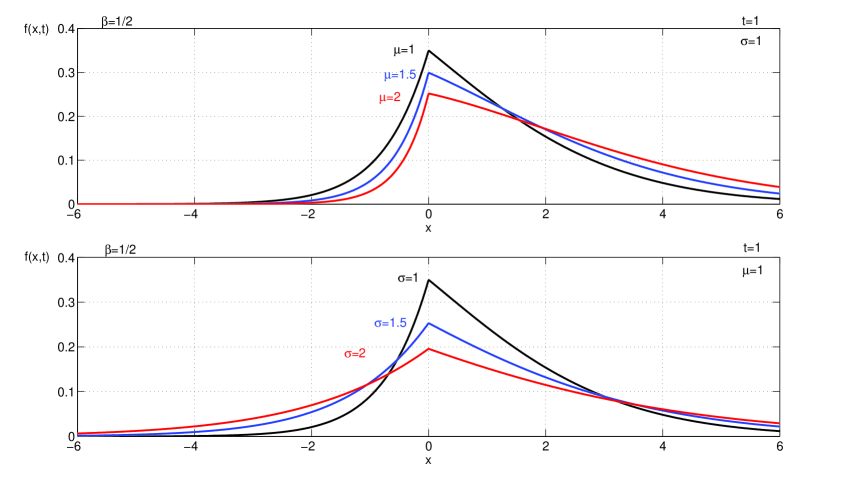
The fundamental solution of Eq. (111) is:

fD​(x,t)=∫0∞fB(ΞΌ)​(x,Ο„)​flβ​(Ο„,t)​𝑑τ,tβ‰₯0,xβˆˆβ„,formulae-sequencesubscript𝑓𝐷π‘₯𝑑superscriptsubscript0subscript𝑓superscriptπ΅πœ‡π‘₯𝜏subscript𝑓subscriptπ‘™π›½πœπ‘‘differential-d𝜏formulae-sequence𝑑0π‘₯ℝf_{D}(x,t)=\int_{0}^{\infty}f_{B^{(\mu)}}(x,\tau)f_{l_{\beta}}(\tau,t)\,d\tau,\;\;t\geq 0,\;\;\ x\in\mathbb{R},

i.e.

fD​(x,t)=∫0∞1|Οƒ|​4​π​τ​exp⁑(βˆ’(xβˆ’ΞΌβ€‹Ο„)24​σ2​τ)​ℳβ​(Ο„,t)​𝑑τ,tβ‰₯0,xβˆˆβ„,formulae-sequencesubscript𝑓𝐷π‘₯𝑑superscriptsubscript01𝜎4πœ‹πœsuperscriptπ‘₯πœ‡πœ24superscript𝜎2𝜏subscriptβ„³π›½πœπ‘‘differential-d𝜏formulae-sequence𝑑0π‘₯ℝf_{D}(x,t)=\int_{0}^{\infty}\frac{1}{|\sigma|\sqrt{4\pi\tau}}\exp\left(-\frac{(x-\mu\tau)^{2}}{4\sigma^{2}\tau}\right)\mathcal{M}_{\beta}(\tau,t)d\tau,\;\;t\geq 0,\;\;x\in\mathbb{R}, (113)

which is equal to:

fD​(x,t)=eμ​x/2​σ2​12​|Οƒ|β€‹βˆ‘k=0∞(βˆ’ΞΌ2​tΞ²/4​σ2)kk!​tβˆ’Ξ²/2​H2,22,0​(|xβ€‹Οƒβˆ’1|​tβˆ’Ξ²/2|(1/2,1/2),(1βˆ’Ξ²/2+β​k,Ξ²/2)(0,1),(k+1/2,1/2)),subscript𝑓𝐷π‘₯𝑑superscriptπ‘’πœ‡π‘₯2superscript𝜎212𝜎superscriptsubscriptπ‘˜0superscriptsuperscriptπœ‡2superscript𝑑𝛽4superscript𝜎2π‘˜π‘˜superscript𝑑𝛽2subscriptsuperscript𝐻2022conditionalπ‘₯superscript𝜎1superscript𝑑𝛽212121𝛽2π›½π‘˜π›½201π‘˜1212f_{D}(x,t)=e^{\mu x/2\sigma^{2}}\frac{1}{2|\sigma|}\sum_{k=0}^{\infty}\frac{(-\mu^{2}t^{\beta}/4\sigma^{2})^{k}}{k!}t^{-\beta/2}H^{2,0}_{2,2}\left(|x\sigma^{-1}|t^{-\beta/2}\Big{|}\begin{array}[]{c}(1/2,1/2),(1-\beta/2+\beta k,\beta/2)\\ (0,1),(k+1/2,1/2)\end{array}\right), (114)

where the Fox H𝐻H-function is defined by Eq. (67).

Refer to caption
Figure 12: Plot of the fundamental solution f​(x,t)𝑓π‘₯𝑑f(x,t), Eq. (114), with Ξ²=1/2𝛽12\beta=1/2, at time t=1𝑑1t=1, for different values of the parameters ΞΌ=[1,1.5,2]πœ‡11.52\mu=[1,1.5,2] and Οƒ=[1,1.5,2]𝜎11.52\sigma=[1,1.5,2].

Proof: In order to evaluate fD​(x,t)subscript𝑓𝐷π‘₯𝑑f_{D}(x,t) we write:

fD​(x,t)=|Οƒ|βˆ’1​eμ​xβ€²/2β€‹Οƒβ€‹βˆ«0∞eβˆ’ΞΌ2​τ/4​σ2​G​(xβ€²,Ο„)​ℳβ​(Ο„,t)​𝑑τ,subscript𝑓𝐷π‘₯𝑑superscript𝜎1superscriptπ‘’πœ‡superscriptπ‘₯β€²2𝜎superscriptsubscript0superscript𝑒superscriptπœ‡2𝜏4superscript𝜎2𝐺superscriptπ‘₯β€²πœsubscriptβ„³π›½πœπ‘‘differential-d𝜏f_{D}(x,t)=|\sigma|^{-1}e^{\mu x^{\prime}/2\sigma}\int_{0}^{\infty}e^{-\mu^{2}\tau/4\sigma^{2}}G(x^{\prime},\tau)\mathcal{M}_{\beta}(\tau,t)d\tau,

where G​(x,t)𝐺π‘₯𝑑G(x,t) is the standard Gaussian density, see Eq. (9) and xβ€²=x/Οƒsuperscriptπ‘₯β€²π‘₯𝜎x^{\prime}=x/\sigma. In view of Eq. (71), we have to evaluate an integral of the form:

Φ​(x,t)=12β€‹βˆ«0∞eβˆ’a​τ​ℳ1/2​(|x|,Ο„)​ℳβ​(Ο„,t)​𝑑τ,xβˆˆβ„,tβ‰₯0,aβ‰₯0.formulae-sequenceΞ¦π‘₯𝑑12superscriptsubscript0superscriptπ‘’π‘Žπœsubscriptβ„³12π‘₯𝜏subscriptβ„³π›½πœπ‘‘differential-d𝜏formulae-sequenceπ‘₯ℝformulae-sequence𝑑0π‘Ž0\Phi(x,t)=\frac{1}{2}\int_{0}^{\infty}e^{-a\tau}\mathcal{M}_{1/2}(|x|,\tau)\mathcal{M}_{\beta}(\tau,t)d\tau,\;\;\ x\in\mathbb{R},\;\;t\geq 0,\;\;a\geq 0. (115)

One has:

Φ​(x,t)=12β€‹βˆ«0∞eβˆ’aβ€‹Ο„β€‹Ο„βˆ’1/2​M1/2​(|x|β€‹Ο„βˆ’1/2)​tβˆ’Ξ²β€‹Mβ​(τ​tβˆ’Ξ²)​𝑑τΦπ‘₯𝑑12superscriptsubscript0superscriptπ‘’π‘Žπœsuperscript𝜏12subscript𝑀12π‘₯superscript𝜏12superscript𝑑𝛽subscriptπ‘€π›½πœsuperscript𝑑𝛽differential-d𝜏\Phi(x,t)=\frac{1}{2}\int_{0}^{\infty}e^{-a\tau}\tau^{-1/2}M_{1/2}(|x|\tau^{-1/2})t^{-\beta}M_{\beta}(\tau t^{-\beta})\,d\tau
=12β€‹βˆ«0∞1y​M1/2​(|x|y)​2​y​eβˆ’a​y2​tβˆ’Ξ²β€‹Mβ​(y2​tβˆ’Ξ²)​𝑑y.absent12superscriptsubscript01𝑦subscript𝑀12π‘₯𝑦2𝑦superscriptπ‘’π‘Žsuperscript𝑦2superscript𝑑𝛽subscript𝑀𝛽superscript𝑦2superscript𝑑𝛽differential-d𝑦=\frac{1}{2}\int_{0}^{\infty}\frac{1}{y}M_{1/2}\left(\frac{|x|}{y}\right)2ye^{-ay^{2}}t^{-\beta}M_{\beta}(y^{2}t^{-\beta})\,dy.

after the change of variables y=Ο„π‘¦πœy=\sqrt{\tau}. Because of the symmetry, it is enough to consider only the case xβ‰₯0π‘₯0x\geq 0. We get:

Φ​(x,t)=12​(M1/2⋆Yt)​(x),xβ‰₯0,formulae-sequenceΞ¦π‘₯𝑑12⋆subscript𝑀12subscriptπ‘Œπ‘‘π‘₯π‘₯0\Phi(x,t)=\frac{1}{2}(M_{1/2}\star Y_{t})(x),\;\;\ x\geq 0,

where

(φ⋆ϕ)​(x)=∫0∞1y​φ​(xy)​ϕ​(y)​𝑑yβ‹†πœ‘italic-Ο•π‘₯superscriptsubscript01π‘¦πœ‘π‘₯𝑦italic-ϕ𝑦differential-d𝑦(\varphi\star\phi)(x)=\int_{0}^{\infty}\frac{1}{y}\varphi\left(\frac{x}{y}\right)\phi(y)dy

indicates the Mellin convolution and where:

Yt​(x)=2​x​eβˆ’a​x2​tβˆ’Ξ²β€‹Mβ​(x2​tβˆ’Ξ²),xβ‰₯0,tβ‰₯0.formulae-sequencesubscriptπ‘Œπ‘‘π‘₯2π‘₯superscriptπ‘’π‘Žsuperscriptπ‘₯2superscript𝑑𝛽subscript𝑀𝛽superscriptπ‘₯2superscript𝑑𝛽formulae-sequenceπ‘₯0𝑑0Y_{t}(x)=2xe^{-ax^{2}}t^{-\beta}M_{\beta}(x^{2}t^{-\beta}),\;\;x\geq 0,\;\;\;t\geq 0. (116)
Refer to caption
Figure 13: Plot of the fundamental solution f​(x,t)𝑓π‘₯𝑑f(x,t), Eq. (114) with Ξ²=1/2𝛽12\beta=1/2, ΞΌ=1πœ‡1\mu=1, Οƒ=1𝜎1\sigma=1, at times t=[0.1,1,2]𝑑0.112t=[0.1,1,2].

Using the Mellin convolution theorem we get:

ℳ​{2​Φ​(x,t);x,u}=ℳ​{M1/2​(x);x,u}​ℳ​{Yt​(x);x,u}.β„³2Ξ¦π‘₯𝑑π‘₯𝑒ℳsubscript𝑀12π‘₯π‘₯𝑒ℳsubscriptπ‘Œπ‘‘π‘₯π‘₯𝑒\mathscr{M}\{2\Phi(x,t);x,u\}=\mathscr{M}\{M_{1/2}(x);x,u\}\mathscr{M}\{Y_{t}(x);x,u\}. (117)

Because ofEq. 68) andEq. 67), this can be written as:

ℳ​{2​Φ​(x,t);x,u}=Γ​(u)Γ​(1/2+u/2)​ℳ​{Yt​(x);x,u}.β„³2Ξ¦π‘₯𝑑π‘₯𝑒Γ𝑒Γ12𝑒2β„³subscriptπ‘Œπ‘‘π‘₯π‘₯𝑒\mathscr{M}\{2\Phi(x,t);x,u\}=\frac{\Gamma(u)}{\Gamma(1/2+u/2)}\mathscr{M}\{Y_{t}(x);x,u\}. (118)

We now evaluate:

ℳ​{Yt​(x);x,u}=∫0∞eβˆ’a​x2​2​x​tβˆ’Ξ²β€‹Mβ​(x2​tβˆ’Ξ²)​xuβˆ’1​𝑑x.β„³subscriptπ‘Œπ‘‘π‘₯π‘₯𝑒superscriptsubscript0superscriptπ‘’π‘Žsuperscriptπ‘₯22π‘₯superscript𝑑𝛽subscript𝑀𝛽superscriptπ‘₯2superscript𝑑𝛽superscriptπ‘₯𝑒1differential-dπ‘₯\mathscr{M}\{Y_{t}(x);x,u\}=\int_{0}^{\infty}e^{-ax^{2}}2xt^{-\beta}M_{\beta}(x^{2}t^{-\beta})x^{u-1}\,dx.

After the change of variables x2​tβˆ’Ξ²=zsuperscriptπ‘₯2superscript𝑑𝛽𝑧x^{2}t^{-\beta}=z, we get

ℳ​{Yt​(x);x,u}=∫0∞(z​tΞ²)12​(uβˆ’1)​eβˆ’a​z​tβ​Mβ​(z)​𝑑zβ„³subscriptπ‘Œπ‘‘π‘₯π‘₯𝑒superscriptsubscript0superscript𝑧superscript𝑑𝛽12𝑒1superscriptπ‘’π‘Žπ‘§superscript𝑑𝛽subscript𝑀𝛽𝑧differential-d𝑧\mathscr{M}\{Y_{t}(x);x,u\}=\int_{0}^{\infty}(zt^{\beta})^{\frac{1}{2}(u-1)}e^{-azt^{\beta}}M_{\beta}(z)dz
=tΞ²2​(uβˆ’1)β€‹βˆ‘k=0∞(βˆ’a​tΞ²)kk!β€‹βˆ«0∞zkβˆ’12+u2​Mβ​(z)​𝑑zabsentsuperscript𝑑𝛽2𝑒1superscriptsubscriptπ‘˜0superscriptπ‘Žsuperscriptπ‘‘π›½π‘˜π‘˜superscriptsubscript0superscriptπ‘§π‘˜12𝑒2subscript𝑀𝛽𝑧differential-d𝑧=t^{\frac{\beta}{2}(u-1)}\sum_{k=0}^{\infty}\frac{(-at^{\beta})^{k}}{k!}\int_{0}^{\infty}z^{k-\frac{1}{2}+\frac{u}{2}}M_{\beta}(z)dz
=tΞ²2​(uβˆ’1)β€‹βˆ‘k=0∞(βˆ’a​tΞ²)kk!​ℳ​{Mβ​(x);x,k+1/2+u/2}absentsuperscript𝑑𝛽2𝑒1superscriptsubscriptπ‘˜0superscriptπ‘Žsuperscriptπ‘‘π›½π‘˜π‘˜β„³subscript𝑀𝛽π‘₯π‘₯π‘˜12𝑒2=t^{\frac{\beta}{2}(u-1)}\sum_{k=0}^{\infty}\frac{(-at^{\beta})^{k}}{k!}\mathscr{M}\{M_{\beta}(x);x,k+1/2+u/2\}
=tΞ²2​(uβˆ’1)β€‹βˆ‘k=0∞(βˆ’a​tΞ²)kk!​Γ​(1/2+k+u/2)Γ​(1+β​kβˆ’Ξ²/2+β​u/2),absentsuperscript𝑑𝛽2𝑒1superscriptsubscriptπ‘˜0superscriptπ‘Žsuperscriptπ‘‘π›½π‘˜π‘˜Ξ“12π‘˜π‘’2Ξ“1π›½π‘˜π›½2𝛽𝑒2=t^{\frac{\beta}{2}(u-1)}\sum_{k=0}^{\infty}\frac{(-at^{\beta})^{k}}{k!}\frac{\Gamma(1/2+k+u/2)}{\Gamma(1+\beta k-\beta/2+\beta u/2)},

where we have used Eq. (68) and Eq. (67). Thus:
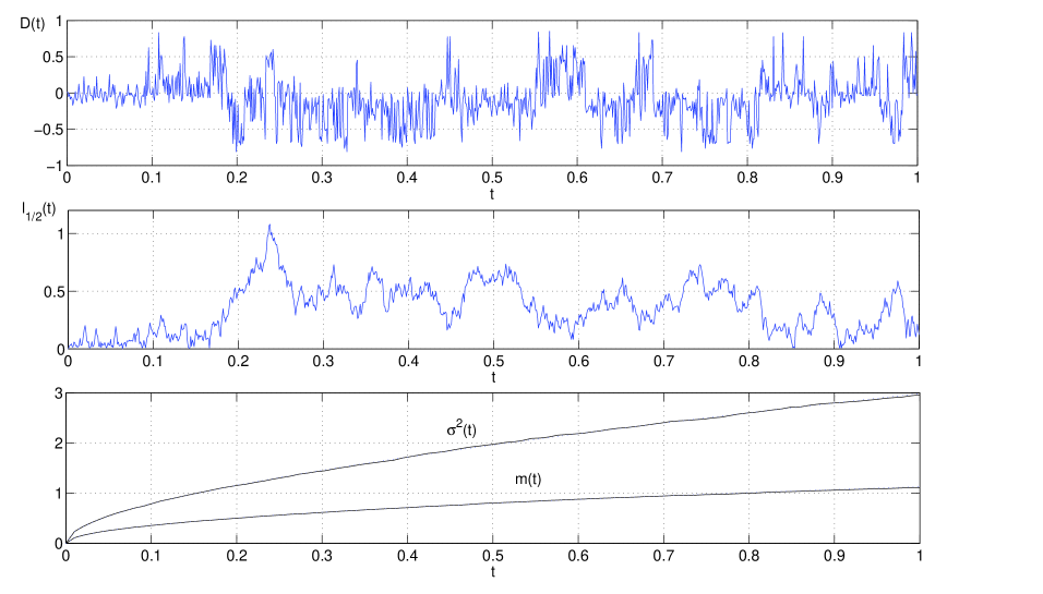
ℳ​{2​Φ​(x,t);x,u}=βˆ‘k=0∞(βˆ’a​tΞ²)kk!​tΞ²2​(uβˆ’1)​Γ​(u)​Γ​(1/2+k+u/2)Γ​(1/2+u/2)​Γ​(1+β​kβˆ’Ξ²/2+β​u/2).β„³2Ξ¦π‘₯𝑑π‘₯𝑒superscriptsubscriptπ‘˜0superscriptπ‘Žsuperscriptπ‘‘π›½π‘˜π‘˜superscript𝑑𝛽2𝑒1Γ𝑒Γ12π‘˜π‘’2Ξ“12𝑒2Ξ“1π›½π‘˜π›½2𝛽𝑒2\mathscr{M}\{2\Phi(x,t);x,u\}=\sum_{k=0}^{\infty}\frac{(-at^{\beta})^{k}}{k!}t^{\frac{\beta}{2}(u-1)}\frac{\Gamma(u)\Gamma(1/2+k+u/2)}{\Gamma(1/2+u/2)\Gamma(1+\beta k-\beta/2+\beta u/2)}.
Refer to caption
Figure 14: Trajectory of the process D​(t)=B(ΞΌ)​(l1/2​(t))𝐷𝑑superscriptπ΅πœ‡subscript𝑙12𝑑D(t)=B^{(\mu)}(l_{1/2}(t)) defined in Eq. 112) with Ξ²=1/2𝛽12\beta=1/2 (top panel). The random time process is l1/2​(t)=|b​(t)|subscript𝑙12𝑑𝑏𝑑l_{1/2}(t)=|b(t)|, where b​(t)𝑏𝑑b(t) is a β€œstandard” Brownian motion (middle panel). The variance and the mean are evaluated over a sample of size N=5β‹…104𝑁⋅5superscript104N=5\cdot 10^{4} and fit the theoretical values (bottom panel).

Inverting the Mellin transform,Eq. 67) gives:

Φ​(x,t)=12β€‹βˆ‘k=0∞(βˆ’a​tΞ²)kk!​tβˆ’Ξ²/2​H2,22,0​(|x|​tβˆ’Ξ²/2|(1/2,1/2),(1βˆ’Ξ²/2+β​k,Ξ²/2)(0,1),(k+1/2,1/2)),Ξ¦π‘₯𝑑12superscriptsubscriptπ‘˜0superscriptπ‘Žsuperscriptπ‘‘π›½π‘˜π‘˜superscript𝑑𝛽2subscriptsuperscript𝐻2022conditionalπ‘₯superscript𝑑𝛽212121𝛽2π›½π‘˜π›½201π‘˜1212\Phi(x,t)=\frac{1}{2}\sum_{k=0}^{\infty}\frac{(-at^{\beta})^{k}}{k!}t^{-\beta/2}H^{2,0}_{2,2}\left(|x|t^{-\beta/2}\Big{|}\begin{array}[]{c}(1/2,1/2),(1-\beta/2+\beta k,\beta/2)\\ (0,1),(k+1/2,1/2)\end{array}\right), (119)

with xβˆˆβ„π‘₯ℝx\in\mathbb{R} and tβ‰₯0𝑑0t\geq 0. Therefore, the fundamental solution of Eq. (103) can be expressed as:

fD​(x,t)=eμ​x/2​σ2​12​|Οƒ|β€‹βˆ‘k=0∞(βˆ’ΞΌ2​tΞ²/4​σ2)kk!​tβˆ’Ξ²/2​H2,22,0​(|xβ€‹Οƒβˆ’1|​tβˆ’Ξ²/2|(1/2,1/2),(1βˆ’Ξ²/2+β​k,Ξ²/2)(0,1),(k+1/2,1/2)),subscript𝑓𝐷π‘₯𝑑superscriptπ‘’πœ‡π‘₯2superscript𝜎212𝜎superscriptsubscriptπ‘˜0superscriptsuperscriptπœ‡2superscript𝑑𝛽4superscript𝜎2π‘˜π‘˜superscript𝑑𝛽2subscriptsuperscript𝐻2022conditionalπ‘₯superscript𝜎1superscript𝑑𝛽212121𝛽2π›½π‘˜π›½201π‘˜1212f_{D}(x,t)=e^{\mu x/2\sigma^{2}}\frac{1}{2|\sigma|}\sum_{k=0}^{\infty}\frac{(-\mu^{2}t^{\beta}/4\sigma^{2})^{k}}{k!}t^{-\beta/2}H^{2,0}_{2,2}\left(|x\sigma^{-1}|t^{-\beta/2}\Big{|}\begin{array}[]{c}(1/2,1/2),(1-\beta/2+\beta k,\beta/2)\\ (0,1),(k+1/2,1/2)\end{array}\right),

that is Eq. (114). β–‘β–‘\Box

When ΞΌ=0πœ‡0\mu=0 and Οƒ=1𝜎1\sigma=1,Eq. 114) reduces to:

fD​(x,t)=12​tβˆ’Ξ²/2​H2,22,0​(|x|​tβˆ’Ξ²/2|(1/2,1/2),(1βˆ’Ξ²/2,Ξ²/2)(0,1),(1/2,1/2)),subscript𝑓𝐷π‘₯𝑑12superscript𝑑𝛽2subscriptsuperscript𝐻2022conditionalπ‘₯superscript𝑑𝛽212121𝛽2𝛽2011212f_{D}(x,t)=\frac{1}{2}t^{-\beta/2}H^{2,0}_{2,2}\left(|x|t^{-\beta/2}\Big{|}\begin{array}[]{c}(1/2,1/2),(1-\beta/2,\beta/2)\\ (0,1),(1/2,1/2)\end{array}\right),

that is, using the reduction formula for the Fox H𝐻H-function [30],

fD​(x,t)=12​tβˆ’Ξ²/2​H1,11,0​(|x|​tβˆ’Ξ²/2|(1βˆ’Ξ²/2,Ξ²/2)(0,1))=12​ℳβ/2​(|x|,t).subscript𝑓𝐷π‘₯𝑑12superscript𝑑𝛽2subscriptsuperscript𝐻1011conditionalπ‘₯superscript𝑑𝛽21𝛽2𝛽20112subscriptℳ𝛽2π‘₯𝑑f_{D}(x,t)=\frac{1}{2}t^{-\beta/2}H^{1,0}_{1,1}\left(|x|t^{-\beta/2}\Big{|}\begin{array}[]{c}(1-\beta/2,\beta/2)\\ (0,1)\end{array}\right)=\frac{1}{2}\mathcal{M}_{\beta/2}(|x|,t).

As expected, we recover in this case the fundamental solution of the time-fractional diffusion equation (72).
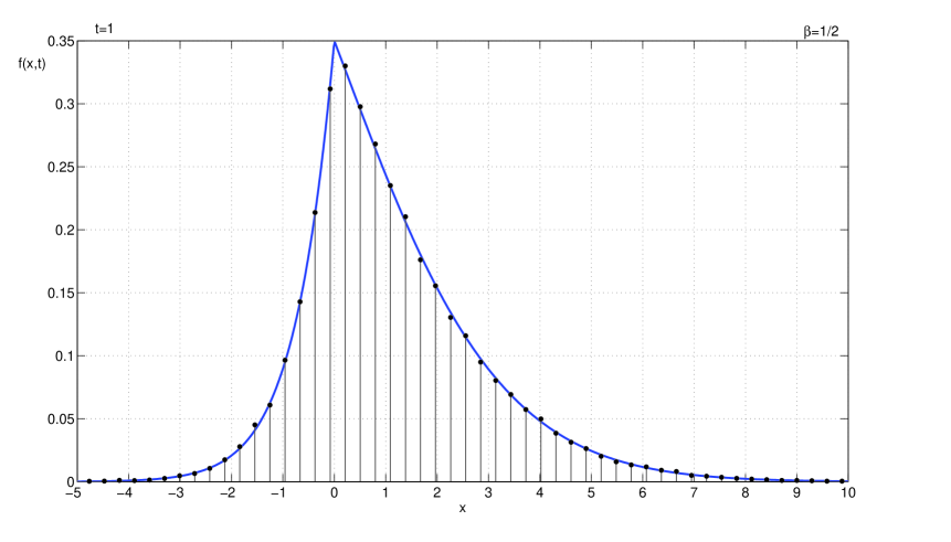
Moreover, if we set Ξ²=1𝛽1\beta=1 in Eq. (114) we have:

fD​(x,t)=eμ​x/2​σ2​12​|Οƒ|β€‹βˆ‘k=0∞(βˆ’ΞΌ2​t/4​σ2)kk!​tβˆ’1/2​H2,22,0​(|xβ€‹Οƒβˆ’1|​tβˆ’1/2|(1/2,1/2),(1/2+k,1/2)(0,1),(1/2+k,1/2)),subscript𝑓𝐷π‘₯𝑑superscriptπ‘’πœ‡π‘₯2superscript𝜎212𝜎superscriptsubscriptπ‘˜0superscriptsuperscriptπœ‡2𝑑4superscript𝜎2π‘˜π‘˜superscript𝑑12subscriptsuperscript𝐻2022conditionalπ‘₯superscript𝜎1superscript𝑑12121212π‘˜120112π‘˜12f_{D}(x,t)=e^{\mu x/2\sigma^{2}}\frac{1}{2|\sigma|}\sum_{k=0}^{\infty}\frac{(-\mu^{2}t/4\sigma^{2})^{k}}{k!}t^{-1/2}H^{2,0}_{2,2}\left(|x\sigma^{-1}|t^{-1/2}\Big{|}\begin{array}[]{c}(1/2,1/2),(1/2+k,1/2)\\ (0,1),(1/2+k,1/2)\end{array}\right),
=eμ​x/2​σ2β€‹βˆ‘k=0∞(βˆ’ΞΌ2​t/4​σ2)kk!​12​|Οƒ|​tβˆ’1/2​H1,11,0​(|xβ€‹Οƒβˆ’1|​tβˆ’1/2|(1/2,1/2)(0,1))=1|Οƒ|​4​π​t​exp⁑(βˆ’(xβˆ’ΞΌβ€‹t)24​σ2​t),absentsuperscriptπ‘’πœ‡π‘₯2superscript𝜎2superscriptsubscriptπ‘˜0superscriptsuperscriptπœ‡2𝑑4superscript𝜎2π‘˜π‘˜12𝜎superscript𝑑12subscriptsuperscript𝐻1011conditionalπ‘₯superscript𝜎1superscript𝑑121212011𝜎4πœ‹π‘‘superscriptπ‘₯πœ‡π‘‘24superscript𝜎2𝑑=e^{\mu x/2\sigma^{2}}\sum_{k=0}^{\infty}\frac{(-\mu^{2}t/4\sigma^{2})^{k}}{k!}\frac{1}{2|\sigma|}t^{-1/2}H^{1,0}_{1,1}\left(|x\sigma^{-1}|t^{-1/2}\Big{|}\begin{array}[]{c}(1/2,1/2)\\ (0,1)\end{array}\right)=\frac{1}{|\sigma|\sqrt{4\pi t}}\exp\left(-\frac{(x-\mu t)^{2}}{4\sigma^{2}t}\right),

and we recover fB(ΞΌ)​(x,t)subscript𝑓superscriptπ΅πœ‡π‘₯𝑑f_{B^{(\mu)}}(x,t).

Refer to caption
Figure 15: Marginal density function f​(x,t)𝑓π‘₯𝑑f(x,t) of the process B(ΞΌ)​(l1/2​(t))superscriptπ΅πœ‡subscript𝑙12𝑑B^{(\mu)}(l_{1/2}(t)) at time t=1𝑑1t=1Eq. 114). The histogram is evaluated over N=105𝑁superscript105N=10^{5} simulated trajectories (see Figure 14).

In Figure 12 and Figure 13 we have used Eq. (113) to plot the fundamental solution (114) with Ξ²=1/2𝛽12\beta=1/2 for different values of the parameters ΞΌπœ‡\mu and ΟƒπœŽ\sigma at fixed time and, for fixed parameters, at different times t𝑑t. As expected, the fundamental solution is not symmetric in space with a time-growing skewness. Moreover, due to the presence of the positively taken drift term (ΞΌ=1πœ‡1\mu=1), the probability to find the particle in the positive semi-axis increases with time (fig. 13).

In Figure 14 is presented a trajectory of the process D​(t)=B(ΞΌ)​(lβ​(t))𝐷𝑑superscriptπ΅πœ‡subscript𝑙𝛽𝑑D(t)=B^{(\mu)}(l_{\beta}(t)) with Ξ²=1/2𝛽12\beta=1/2. Using Eq. (73) it is easy to write all the moments of the process:

E​(D​(t)m)=βˆ‘k=0[m/2](m2​k)​2​k!​(mβˆ’k)!k!​σ2​k​μmβˆ’2​k​tβ​(mβˆ’k)Γ​(β​(mβˆ’k)+1),  0<β≀1,formulae-sequence𝐸𝐷superscriptπ‘‘π‘šsuperscriptsubscriptπ‘˜0delimited-[]π‘š2π‘šmissing-subexpression2π‘˜missing-subexpression2π‘˜π‘šπ‘˜π‘˜superscript𝜎2π‘˜superscriptπœ‡π‘š2π‘˜superscriptπ‘‘π›½π‘šπ‘˜Ξ“π›½π‘šπ‘˜1  0𝛽1E(D(t)^{m})=\sum_{k=0}^{[m/2]}\left(\!\!\begin{array}[]{cc}m\\ 2k\end{array}\!\!\right)\frac{2k!(m-k)!}{k!}\sigma^{2k}\mu^{m-2k}\frac{t^{\beta(m-k)}}{\Gamma(\beta(m-k)+1)},\;\;0<\beta\leq 1, (120)

where mπ‘šm is an integer greater than zero and [a]delimited-[]π‘Ž[a] indicates the integer part of aπ‘Ža. Therefore, we have:

m​(t)=E​(D​(t))=μ​tβΓ​(Ξ²+1),π‘šπ‘‘πΈπ·π‘‘πœ‡superscript𝑑𝛽Γ𝛽1m(t)=E(D(t))=\mu\frac{t^{\beta}}{\Gamma(\beta+1)}, (121)

and

Οƒ2​(t)=E​(D​(t)2)βˆ’m​(t)2=2​μ2​t2​βΓ​(2​β+1)βˆ’ΞΌ2​t2​βΓ​(Ξ²+1)2+2​σ2​tβΓ​(Ξ²+1).superscript𝜎2𝑑𝐸𝐷superscript𝑑2π‘šsuperscript𝑑22superscriptπœ‡2superscript𝑑2𝛽Γ2𝛽1superscriptπœ‡2superscript𝑑2𝛽Γsuperscript𝛽122superscript𝜎2superscript𝑑𝛽Γ𝛽1\sigma^{2}(t)=E(D(t)^{2})-m(t)^{2}=2\mu^{2}\frac{t^{2\beta}}{\Gamma(2\beta+1)}-\mu^{2}\frac{t^{2\beta}}{\Gamma(\beta+1)^{2}}+2\sigma^{2}\frac{t^{\beta}}{\Gamma(\beta+1)}. (122)

In the bottom panel of Figure 14 the mean and the variance have been estimated from a sample of trajectories of the process B(ΞΌ)​(l1/2)​(t)superscriptπ΅πœ‡subscript𝑙12𝑑B^{(\mu)}(l_{1/2})(t). Then, they have been compared with the theoretical values given above. In Figure 15 we compare the theoretical density function f​(x,t)𝑓π‘₯𝑑f(x,t) given by Eq. 114) at time t=1𝑑1t=1 with an histogram evaluated over a sample of N=105𝑁superscript105N=10^{5} trajectories.

8.1.2 Exponential-decay kernel

The exponential-decay kernel case is straightforward. The non-Markovian Fokker-Planck equation is:

u​(x,t)=u0​(x)+∫0teβˆ’a​(tβˆ’s)​(βˆ’ΞΌβ€‹βˆ‚xu​(x,s)+Οƒ2β€‹βˆ‚x​xu​(x,s))​𝑑s,aβ‰₯0.formulae-sequence𝑒π‘₯𝑑subscript𝑒0π‘₯superscriptsubscript0𝑑superscriptπ‘’π‘Žπ‘‘π‘ πœ‡subscriptπ‘₯𝑒π‘₯𝑠superscript𝜎2subscriptπ‘₯π‘₯𝑒π‘₯𝑠differential-dπ‘ π‘Ž0u(x,t)=u_{0}(x)+\int_{0}^{t}e^{-a(t-s)}(-\mu\partial_{x}u(x,s)+\sigma^{2}\partial_{xx}u(x,s))ds,\;\;a\geq 0. (123)

If we indicate by 𝒒​(x,t)𝒒π‘₯𝑑\mathcal{G}(x,t) the fundamental solution of the Markovian equation; i.e. Eq. (109)

𝒒​(x,t)=1|Οƒ|​4​π​t​exp⁑(βˆ’(xβˆ’ΞΌβ€‹t)24​σ2​t),tβ‰₯0,xβˆˆβ„,formulae-sequence𝒒π‘₯𝑑1𝜎4πœ‹π‘‘superscriptπ‘₯πœ‡π‘‘24superscript𝜎2𝑑formulae-sequence𝑑0π‘₯ℝ\mathcal{G}(x,t)=\frac{1}{|\sigma|\sqrt{4\pi t}}\exp\left(-\frac{(x-\mu t)^{2}}{4\sigma^{2}t}\right),\;\;t\geq 0,\;\;x\in\mathbb{R}, (124)

then, using Eq. (82), the fundamental solution of Eq. (123) is:

f​(x,t)=eβˆ’a​t​𝒒​(x,t)+(1βˆ’eβˆ’a​t)​Φ​(x,t),𝑓π‘₯𝑑superscriptπ‘’π‘Žπ‘‘π’’π‘₯𝑑1superscriptπ‘’π‘Žπ‘‘Ξ¦π‘₯𝑑f(x,t)=e^{-at}\mathcal{G}(x,t)+(1-e^{-at})\Phi(x,t), (125)

where:

Φ​(x,t)=a1βˆ’eβˆ’a​t​eμ​x/2​σ2β€‹βˆ«0teβˆ’x2/4​σ2​τ​eβˆ’(a+ΞΌ2/4​σ2)​τ|Οƒ|​4​π​τ​𝑑τ.Ξ¦π‘₯π‘‘π‘Ž1superscriptπ‘’π‘Žπ‘‘superscriptπ‘’πœ‡π‘₯2superscript𝜎2superscriptsubscript0𝑑superscript𝑒superscriptπ‘₯24superscript𝜎2𝜏superscriptπ‘’π‘Žsuperscriptπœ‡24superscript𝜎2𝜏𝜎4πœ‹πœdifferential-d𝜏\Phi(x,t)=\frac{a}{1-e^{-at}}e^{\mu x/2\sigma^{2}}\int_{0}^{t}\frac{e^{-x^{2}/4\sigma^{2}\tau}e^{-(a+\mu^{2}/4\sigma^{2})\tau}}{|\sigma|\sqrt{4\pi\tau}}\,d\tau.

Using Eq. (91) and Eq. (93) we have:

Proposition 8.2.

The fundamental solution of Eq. (123) is:

f​(x,t)=eβˆ’a​t​𝒒​(x,t)βˆ’a​eΞΌ2​σ2​x2​|Οƒ|​a+ΞΌ24​σ2​sinh⁑(|xβ€‹Οƒβˆ’1|​a+ΞΌ24​σ2)+𝑓π‘₯𝑑superscriptπ‘’π‘Žπ‘‘π’’π‘₯𝑑limit-fromπ‘Žsuperscriptπ‘’πœ‡2superscript𝜎2π‘₯2πœŽπ‘Žsuperscriptπœ‡24superscript𝜎2π‘₯superscript𝜎1π‘Žsuperscriptπœ‡24superscript𝜎2f(x,t)=e^{-at}\mathcal{G}(x,t)-\frac{ae^{\frac{\mu}{2\sigma^{2}}x}}{2|\sigma|\sqrt{a+\frac{\mu^{2}}{4\sigma^{2}}}}\sinh\left(|x\sigma^{-1}|\sqrt{a+\frac{\mu^{2}}{4\sigma^{2}}}\right)+
+a​eΞΌ2​σ2​x4​|Οƒ|​a+ΞΌ24​σ2{exp(x|Οƒ|a+ΞΌ24​σ2)Erf(x2​|Οƒ|​t+(a+ΞΌ24​σ2)​t)+\frac{ae^{\frac{\mu}{2\sigma^{2}}x}}{4|\sigma|\sqrt{a+\frac{\mu^{2}}{4\sigma^{2}}}}\left\{\exp\left(\frac{x}{|\sigma|}\sqrt{a+\frac{\mu^{2}}{4\sigma^{2}}}\right)\textrm{\rm Erf}\left(\frac{x}{2|\sigma|\sqrt{t}}+\sqrt{\Big{(}a+\frac{\mu^{2}}{4\sigma^{2}}\Big{)}t}\right)\right.
βˆ’exp(βˆ’x|Οƒ|a+ΞΌ24​σ2)Erf(x2​|Οƒ|​tβˆ’(a+ΞΌ24​σ2)​t)}.\left.-\exp\left(-\frac{x}{|\sigma|}\sqrt{a+\frac{\mu^{2}}{4\sigma^{2}}}\right)\textrm{\rm Erf}\left(\frac{x}{2|\sigma|\sqrt{t}}-\sqrt{\Big{(}a+\frac{\mu^{2}}{4\sigma^{2}}\Big{)}t}\right)\right\}. (126)

When tβ†’βˆžβ†’π‘‘t\rightarrow\infty we obtain the stationary distribution:

ϕ¯​(x)=a​eΞΌ2​σ2​x2​|Οƒ|​a+ΞΌ24​σ2​(cosh⁑(x​|Οƒβˆ’1|​a+ΞΌ24​σ2)βˆ’sinh⁑(|xβ€‹Οƒβˆ’1|​a+ΞΌ24​σ2))Β―italic-Ο•π‘₯π‘Žsuperscriptπ‘’πœ‡2superscript𝜎2π‘₯2πœŽπ‘Žsuperscriptπœ‡24superscript𝜎2π‘₯superscript𝜎1π‘Žsuperscriptπœ‡24superscript𝜎2π‘₯superscript𝜎1π‘Žsuperscriptπœ‡24superscript𝜎2\overline{\phi}(x)=\frac{ae^{\frac{\mu}{2\sigma^{2}}x}}{2|\sigma|\sqrt{a+\frac{\mu^{2}}{4\sigma^{2}}}}\left(\cosh\left(x|\sigma^{-1}|\sqrt{a+\frac{\mu^{2}}{4\sigma^{2}}}\right)-\sinh\left(|x\sigma^{-1}|\sqrt{a+\frac{\mu^{2}}{4\sigma^{2}}}\right)\right)

that is:

ϕ¯​(x)=a2​|Οƒ|​a+ΞΌ24​σ2​exp⁑(μ​x/2​σ2βˆ’|xβ€‹Οƒβˆ’1|​a+ΞΌ24​σ2).Β―italic-Ο•π‘₯π‘Ž2πœŽπ‘Žsuperscriptπœ‡24superscript𝜎2πœ‡π‘₯2superscript𝜎2π‘₯superscript𝜎1π‘Žsuperscriptπœ‡24superscript𝜎2\overline{\phi}(x)=\frac{a}{2|\sigma|\sqrt{a+\frac{\mu^{2}}{4\sigma^{2}}}}\exp\left(\mu x/2\sigma^{2}-|x\sigma^{-1}|\sqrt{a+\frac{\mu^{2}}{4\sigma^{2}}}\right). (127)

8.2 Geometric Brownian motion

Let ΞΌβˆˆβ„πœ‡β„\mu\in\mathbb{R} and Οƒ2>0superscript𝜎20\sigma^{2}>0 be given. Consider a linear diffusion S𝑆S on ℝℝ\mathbb{R} defined by the stochastic differential equation:

d​S​(t)=μ​S​(t)​d​t+σ​S​(t)​d​B​(t),tβ‰₯0,formulae-sequenceπ‘‘π‘†π‘‘πœ‡π‘†π‘‘π‘‘π‘‘πœŽπ‘†π‘‘π‘‘π΅π‘‘π‘‘0dS(t)=\mu S(t)dt+\sigma S(t)dB(t),\;\;t\geq 0, (128)

where B​(t)𝐡𝑑B(t), tβ‰₯0𝑑0t\geq 0, is a β€œstandard” Brownian motion. The process S​(t)𝑆𝑑S(t), tβ‰₯0𝑑0t\geq 0, is called Geometric Brownian motion. If S𝑆S starts in x0subscriptπ‘₯0x_{0} at time t=0𝑑0t=0 (i.e. P​(S​(0)=x0)=1𝑃𝑆0subscriptπ‘₯01P(S(0)=x_{0})=1), then a solution of Eq. (128) is:

S​(t)=x0​exp⁑[(ΞΌβˆ’Οƒ2/2)​t+σ​B​(t)],tβ‰₯0,x0>0.formulae-sequence𝑆𝑑subscriptπ‘₯0πœ‡superscript𝜎22π‘‘πœŽπ΅π‘‘formulae-sequence𝑑0subscriptπ‘₯00S(t)=x_{0}\exp\left[(\mu-\sigma^{2}/2)t+\sigma B(t)\right],\;\;t\geq 0,\;\;x_{0}>0. (129)

The marginal density function of S​(t)𝑆𝑑S(t) is the log-normal distribution:

fS​(x,t)=1x​|Οƒ|​4​π​t​exp⁑(βˆ’(log⁑(x/x0)βˆ’(ΞΌβˆ’Οƒ2/2)​t)2Οƒ2​4​t),tβ‰₯0,xβ‰₯0.formulae-sequencesubscript𝑓𝑆π‘₯𝑑1π‘₯𝜎4πœ‹π‘‘superscriptπ‘₯subscriptπ‘₯0πœ‡superscript𝜎22𝑑2superscript𝜎24𝑑formulae-sequence𝑑0π‘₯0f_{S}(x,t)=\frac{1}{x|\sigma|\sqrt{4\pi t}}\exp\left(-\frac{\Big{(}\log(x/x_{0})-(\mu-\sigma^{2}/2)t\Big{)}^{2}}{\sigma^{2}4t}\right),\;\;t\geq 0,\;\,x\geq 0. (130)

The function fS​(x,t)subscript𝑓𝑆π‘₯𝑑f_{S}(x,t) is a solution of the Fokker-Planck equation:

βˆ‚tu​(x,t)=[(2​σ2βˆ’ΞΌ)+(4​σ2βˆ’ΞΌ)​xβ€‹βˆ‚x+Οƒ2​x2β€‹βˆ‚x​x]​u​(x,t),xβ‰₯0,formulae-sequencesubscript𝑑𝑒π‘₯𝑑delimited-[]2superscript𝜎2πœ‡4superscript𝜎2πœ‡π‘₯subscriptπ‘₯superscript𝜎2superscriptπ‘₯2subscriptπ‘₯π‘₯𝑒π‘₯𝑑π‘₯0\partial_{t}u(x,t)=\left[(2\sigma^{2}-\mu)+(4\sigma^{2}-\mu)x\partial_{x}+\sigma^{2}x^{2}\partial_{xx}\right]u(x,t),\;\;x\geq 0, (131)

with deterministic initial condition

u0​(x)=δ​(xβˆ’x0),xβ‰₯0,x0>0.formulae-sequencesubscript𝑒0π‘₯𝛿π‘₯subscriptπ‘₯0formulae-sequenceπ‘₯0subscriptπ‘₯00u_{0}(x)=\delta(x-x_{0}),\;\;\ x\geq 0,\;\;x_{0}>0. (132)

8.2.1 β𝛽\beta-power kernel

If we introduce the β𝛽\beta-power kernel K​(t)=Γ​(Ξ²)βˆ’1​tΞ²βˆ’1𝐾𝑑Γsuperscript𝛽1superscript𝑑𝛽1K(t)=\Gamma(\beta)^{-1}t^{\beta-1}, 0<β≀10𝛽10<\beta\leq 1, in this setting we obtain the following β€œfractional” Fokker-Planck equation:

u​(x,t)=u0​(x)+1Γ​(Ξ²)β€‹βˆ«0t(tβˆ’s)Ξ²βˆ’1​[(2​σ2βˆ’ΞΌ)+(4​σ2βˆ’ΞΌ)​xβ€‹βˆ‚x+Οƒ2​x2β€‹βˆ‚x​x]​u​(x,s)​𝑑s,xβ‰₯0.formulae-sequence𝑒π‘₯𝑑subscript𝑒0π‘₯1Γ𝛽superscriptsubscript0𝑑superscript𝑑𝑠𝛽1delimited-[]2superscript𝜎2πœ‡4superscript𝜎2πœ‡π‘₯subscriptπ‘₯superscript𝜎2superscriptπ‘₯2subscriptπ‘₯π‘₯𝑒π‘₯𝑠differential-d𝑠π‘₯0u(x,t)=u_{0}(x)+\frac{1}{\Gamma(\beta)}\int_{0}^{t}\left(t-s\right)^{\beta-1}\left[(2\sigma^{2}-\mu)+(4\sigma^{2}-\mu)x\partial_{x}+\sigma^{2}x^{2}\partial_{xx}\right]u(x,s)ds,\;\;x\geq 0. (133)

A solution of the above equation with initial condition given by Eq. (132) is given by (see Corollary 6.1):

fD​(x,t)=∫0∞fS​(x,Ο„)​ℳβ​(Ο„,t)​𝑑τsubscript𝑓𝐷π‘₯𝑑superscriptsubscript0subscript𝑓𝑆π‘₯𝜏subscriptβ„³π›½πœπ‘‘differential-d𝜏f_{D}(x,t)=\int_{0}^{\infty}f_{S}(x,\tau)\mathcal{M}_{\beta}(\tau,t)d\tau (134)

which is the marginal distribution of the process

D​(t)=S​(lβ​(t)),tβ‰₯0,  0<β≀1,formulae-sequence𝐷𝑑𝑆subscript𝑙𝛽𝑑formulae-sequence𝑑0  0𝛽1D(t)=S(l_{\beta}(t)),\;\;t\geq 0,\;\;0<\beta\leq 1, (135)

starting almost surely in x0>0subscriptπ‘₯00x_{0}>0, where lβ​(t)subscript𝑙𝛽𝑑l_{\beta}(t), tβ‰₯0𝑑0t\geq 0, is a self-similar random time process with H=Ξ²/2𝐻𝛽2H=\beta/2, independent of the geometric Brownian motion S​(t)𝑆𝑑S(t) and with marginal density function given by Eq. (105). It is easy to see that:

fD​(x,t)=1x​|Οƒ|​exp⁑(log⁑(x/x0)​(ΞΌβˆ’Οƒ2/2)4​σ2)​12β€‹βˆ«0∞eβˆ’a​τ​ℳ1/2​(|xβ€²|,Ο„)​ℳβ​(Ο„,t)​𝑑τ,subscript𝑓𝐷π‘₯𝑑1π‘₯𝜎π‘₯subscriptπ‘₯0πœ‡superscript𝜎224superscript𝜎212superscriptsubscript0superscriptπ‘’π‘Žπœsubscriptβ„³12superscriptπ‘₯β€²πœsubscriptβ„³π›½πœπ‘‘differential-d𝜏f_{D}(x,t)=\frac{1}{x|\sigma|}\exp{\left(\frac{\log(x/x_{0})(\mu-\sigma^{2}/2)}{4\sigma^{2}}\right)}\frac{1}{2}\int_{0}^{\infty}e^{-a\tau}\mathcal{M}_{1/2}(|x^{\prime}|,\tau)\mathcal{M}_{\beta}(\tau,t)\,d\tau,

where:

a=(ΞΌβˆ’Οƒ2/2)2/4​σ2,xβ€²=log⁑(x/x0)/Οƒ.formulae-sequenceπ‘Žsuperscriptπœ‡superscript𝜎2224superscript𝜎2superscriptπ‘₯β€²π‘₯subscriptπ‘₯0𝜎a=(\mu-\sigma^{2}/2)^{2}/4\sigma^{2},\;\;x^{\prime}=\log(x/x_{0})/\sigma.

We have the same integral as in Eq. (115). Therefore:

Proposition 8.3.

for each tβ‰₯0𝑑0t\geq 0:

fD(x,t)=1x​|Οƒ|exp(log⁑(x/x0)​(ΞΌβˆ’Οƒ2/2)4​σ2)Γ—f_{D}(x,t)=\frac{1}{x|\sigma|}\exp\left(\frac{\log(x/x_{0})(\mu-\sigma^{2}/2)}{4\sigma^{2}}\right)\times
Γ—βˆ‘k=0∞1k!(βˆ’(ΞΌβˆ’Οƒ2/2)2​tΞ²4​σ2)ktβˆ’Ξ²2H2,22,0(|xβ€²|tβˆ’Ξ²2|(1/2,1/2),(1βˆ’Ξ²/2+β​k,Ξ²/2)(0,1),(k+1/2,1/2)).\times\sum_{k=0}^{\infty}\frac{1}{k!}\left(-\frac{(\mu-\sigma^{2}/2)^{2}t^{\beta}}{4\sigma^{2}}\right)^{k}t^{-\frac{\beta}{2}}H^{2,0}_{2,2}\left(|x^{\prime}|t^{-\frac{\beta}{2}}\Big{|}\begin{array}[]{c}(1/2,1/2),(1-\beta/2+\beta k,\beta/2)\\ (0,1),(k+1/2,1/2)\end{array}\right). (136)
Refer to caption
Figure 16: Plot of the fundamental solution f​(x,t)𝑓π‘₯𝑑f(x,t), Eq. (136) at time t=1𝑑1t=1, when ΞΌ=Οƒ2/2=1πœ‡superscript𝜎221\mu=\sigma^{2}/2=1Eq. 137), x0=1subscriptπ‘₯01x_{0}=1, for different values of the parameter Ξ²=[1/4,1/2,3/4,1]𝛽1412341\beta=[1/4,1/2,3/4,1]. For Ξ²=1𝛽1\beta=1 f​(x,t)𝑓π‘₯𝑑f(x,t) reduces to the log-normal density (130). The angular point corresponds to the initial value x0=1subscriptπ‘₯01x_{0}=1 and is due to the presence of |log⁑(x/x0)|π‘₯subscriptπ‘₯0|\log(x/x_{0})| in the solution.

This result can be obtained directly from Eq. (114) because our process is:

D​(t)=x0​exp⁑(B(ΞΌβ€²)​(lβ​(t))),𝐷𝑑subscriptπ‘₯0superscript𝐡superscriptπœ‡β€²subscript𝑙𝛽𝑑D(t)=x_{0}\exp(B^{(\mu^{\prime})}(l_{\beta}(t))),

where B(ΞΌβ€²)superscript𝐡superscriptπœ‡β€²B^{(\mu^{\prime})} is a Brownian motion with drift ΞΌβ€²=(ΞΌβˆ’Οƒ2/2)superscriptπœ‡β€²πœ‡superscript𝜎22\mu^{\prime}=(\mu-\sigma^{2}/2). When Ξ²=1𝛽1\beta=1 we recover Eq. (130). Moreover, if ΞΌ=Οƒ2/2πœ‡superscript𝜎22\mu=\sigma^{2}/2 (i.e. ΞΌβ€²=0superscriptπœ‡β€²0\mu^{\prime}=0) we have (see Figure 16):

fD​(x,t)=1x​|Οƒ|​tβˆ’Ξ²/2​MΞ²/2​(|log⁑(x/x0)Οƒ|​tβˆ’Ξ²/2),xβ‰₯0,tβ‰₯0,formulae-sequencesubscript𝑓𝐷π‘₯𝑑1π‘₯𝜎superscript𝑑𝛽2subscript𝑀𝛽2π‘₯subscriptπ‘₯0𝜎superscript𝑑𝛽2formulae-sequenceπ‘₯0𝑑0f_{D}(x,t)=\frac{1}{x|\sigma|}t^{-\beta/2}M_{\beta/2}\left(\bigg{|}\frac{\log(x/x_{0})}{\sigma}\bigg{|}t^{-\beta/2}\right),\;\;x\geq 0,\;\;t\geq 0, (137)

which is the marginal probability density of:
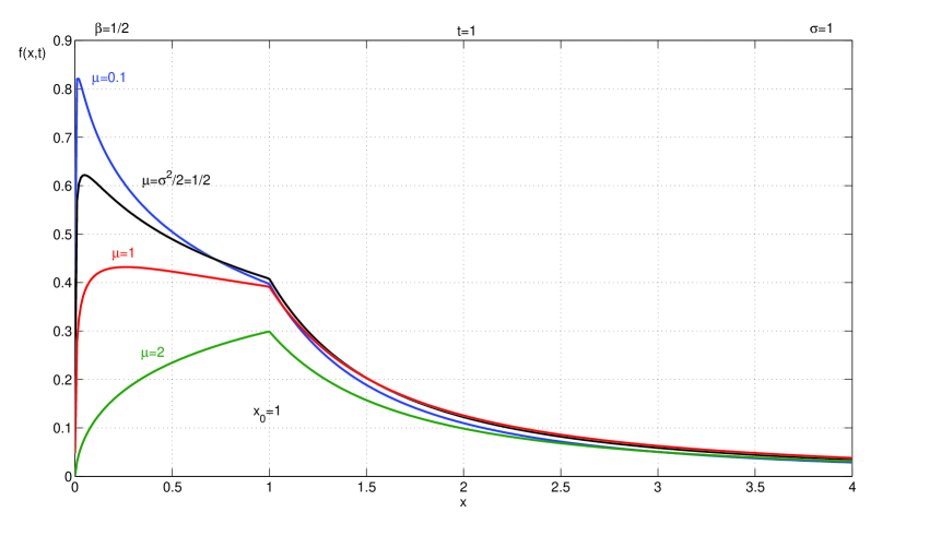
D​(t)=x0​eσ​B​(lβ​(t)),tβ‰₯0.formulae-sequence𝐷𝑑subscriptπ‘₯0superscriptπ‘’πœŽπ΅subscript𝑙𝛽𝑑𝑑0D(t)=x_{0}e^{\sigma B(l_{\beta}(t))},\;\,t\geq 0.
Refer to caption
Figure 17: Plot of the fundamental solution f​(x,t)𝑓π‘₯𝑑f(x,t), Eq. (136), with Ξ²=1/2𝛽12\beta=1/2, Οƒ=1𝜎1\sigma=1, x0=1subscriptπ‘₯01x_{0}=1, at time t=1𝑑1t=1, for different values of the parameter ΞΌ=[0.1,1/2,1,2]πœ‡0.11212\mu=[0.1,1/2,1,2]. For ΞΌ=1/2πœ‡12\mu=1/2 we have Eq. (137), see also Figure 16.
Refer to caption
Figure 18: Plot of the fundamental solution f​(x,t)𝑓π‘₯𝑑f(x,t), Eq. (136), with Ξ²=1/4𝛽14\beta=1/4 (left panel) and Ξ²=1/2𝛽12\beta=1/2 (right panel), at different times t=[0.5,1,2,10]𝑑0.51210t=[0.5,1,2,10].

In Figure 16 we show the plot of the fundamental solution f​(x,t)𝑓π‘₯𝑑f(x,t) in the particular case given by Eq. (137). Here we can see the behavior of the solution varying the parameter β𝛽\beta. For Ξ²=1𝛽1\beta=1 we recover the log-normal density (130) with ΞΌ=Οƒ2/2πœ‡superscript𝜎22\mu=\sigma^{2}/2. In Figure 17 we point out the dependence of the solution with respect to the drift parameter ΞΌπœ‡\mu for fixed Ξ²=1/2𝛽12\beta=1/2, t=1𝑑1t=1, Οƒ=1𝜎1\sigma=1 and x0=1subscriptπ‘₯01x_{0}=1. In Figure 18 we present the time evolution of the fundamental solution with Ξ²=1/2𝛽12\beta=1/2 and Ξ²=1/4𝛽14\beta=1/4.

In Figure 19 we present a trajectory of the process D​(t)=S​(lβ​(t))𝐷𝑑𝑆subscript𝑙𝛽𝑑D(t)=S(l_{\beta}(t)) with Ξ²=1/2𝛽12\beta=1/2, Eq. (135). We shall now compute the mean and the variance of the process D​(t)𝐷𝑑D(t). We have that:

E(S(t))=E(x0exp[(ΞΌβˆ’Οƒ2/2)t+ΟƒB(t))])=x0exp[(ΞΌβˆ’Οƒ2/2)t]E(eσ​B​(t)).E(S(t))=E\left(x_{0}\exp\left[(\mu-\sigma^{2}/2)t+\sigma B(t))\right]\right)=x_{0}\exp\left[(\mu-\sigma^{2}/2)t\right]E\left(e^{\sigma B(t)}\right).

Therefore, because:

E​(eσ​B​(t))=βˆ«β„eσ​x​G​(x,t)​𝑑x=eΟƒ2​t​14​π​tβ€‹βˆ«β„eβˆ’(xβˆ’2​σ​t)24​t​𝑑x,𝐸superscriptπ‘’πœŽπ΅π‘‘subscriptℝsuperscriptπ‘’πœŽπ‘₯𝐺π‘₯𝑑differential-dπ‘₯superscript𝑒superscript𝜎2𝑑14πœ‹π‘‘subscriptℝsuperscript𝑒superscriptπ‘₯2πœŽπ‘‘24𝑑differential-dπ‘₯E(e^{\sigma B(t)})=\int_{\mathbb{R}}e^{\sigma x}G(x,t)dx=e^{\sigma^{2}t}\frac{1}{\sqrt{4\pi t}}\int_{\mathbb{R}}e^{-\frac{(x-2\sigma t)^{2}}{4t}}\,dx,

we have:

E​(S​(t))=x0​exp⁑[(ΞΌ+Οƒ2/2)​t].𝐸𝑆𝑑subscriptπ‘₯0πœ‡superscript𝜎22𝑑E(S(t))=x_{0}\exp\left[(\mu+\sigma^{2}/2)t\right]. (138)

In the same way one has:

E​(S​(t)2)=x02​exp⁑[(2​μ+3​σ2)​t].𝐸𝑆superscript𝑑2superscriptsubscriptπ‘₯022πœ‡3superscript𝜎2𝑑E(S(t)^{2})=x_{0}^{2}\exp\left[(2\mu+3\sigma^{2})t\right]. (139)

Using the above equations we have:

E​(S​(lβ​(t)))=x0​E​(exp⁑[(ΞΌ+Οƒ2/2)​lβ​(t)])=x0β€‹βˆ‘k=0∞(ΞΌ+Οƒ2/2)kk!​E​(lβ​(t)k),𝐸𝑆subscript𝑙𝛽𝑑subscriptπ‘₯0πΈπœ‡superscript𝜎22subscript𝑙𝛽𝑑subscriptπ‘₯0superscriptsubscriptπ‘˜0superscriptπœ‡superscript𝜎22π‘˜π‘˜πΈsubscript𝑙𝛽superscriptπ‘‘π‘˜E(S(l_{\beta}(t)))=x_{0}E\left(\exp\left[(\mu+\sigma^{2}/2)l_{\beta}(t)\right]\right)=x_{0}\sum_{k=0}^{\infty}\frac{(\mu+\sigma^{2}/2)^{k}}{k!}E(l_{\beta}(t)^{k}),

which, using Eq. (73), becomes:

E​(S​(lβ​(t)))=x0β€‹βˆ‘k=0∞((ΞΌ+Οƒ2/2)​tΞ²)kΓ​(β​k+1)=x0​Eβ​((ΞΌ+Οƒ2/2)​tΞ²),𝐸𝑆subscript𝑙𝛽𝑑subscriptπ‘₯0superscriptsubscriptπ‘˜0superscriptπœ‡superscript𝜎22superscriptπ‘‘π›½π‘˜Ξ“π›½π‘˜1subscriptπ‘₯0subscriptπΈπ›½πœ‡superscript𝜎22superscript𝑑𝛽E(S(l_{\beta}(t)))=x_{0}\sum_{k=0}^{\infty}\frac{\left((\mu+\sigma^{2}/2)t^{\beta}\right)^{k}}{\Gamma(\beta k+1)}=x_{0}E_{\beta}((\mu+\sigma^{2}/2)t^{\beta}),

where Eβ​(z)=βˆ‘k=0∞zk/Γ​(β​k+1)subscript𝐸𝛽𝑧superscriptsubscriptπ‘˜0superscriptπ‘§π‘˜Ξ“π›½π‘˜1E_{\beta}(z)=\displaystyle\sum_{k=0}^{\infty}z^{k}/\Gamma(\beta k+1) is the Mittag-Leffler function of order β𝛽\beta [26]. Similarly:

E​(S​(lβ​(t))2)=x02​E​(exp⁑[(2​μ+3​σ2)​lβ​(t)])=x02​Eβ​((2​μ+3​σ2)​tΞ²).𝐸𝑆superscriptsubscript𝑙𝛽𝑑2superscriptsubscriptπ‘₯02𝐸2πœ‡3superscript𝜎2subscript𝑙𝛽𝑑superscriptsubscriptπ‘₯02subscript𝐸𝛽2πœ‡3superscript𝜎2superscript𝑑𝛽E(S(l_{\beta}(t))^{2})=x_{0}^{2}E\left(\exp\left[(2\mu+3\sigma^{2})l_{\beta}(t)\right]\right)=x_{0}^{2}E_{\beta}((2\mu+3\sigma^{2})t^{\beta}).

Finally one has:

{m​(t)=E​(D​(t))=x0​Eβ​((ΞΌ+Οƒ2/2)​tΞ²)Οƒ2​(t)=E​(D​(t)2)βˆ’m​(t)2=x02​[Eβ​((2​μ+3​σ2)​tΞ²)βˆ’Eβ​((ΞΌ+Οƒ2/2)​tΞ²)2]casesπ‘šπ‘‘πΈπ·π‘‘subscriptπ‘₯0subscriptπΈπ›½πœ‡superscript𝜎22superscript𝑑𝛽missing-subexpressionsuperscript𝜎2𝑑𝐸𝐷superscript𝑑2π‘šsuperscript𝑑2superscriptsubscriptπ‘₯02delimited-[]subscript𝐸𝛽2πœ‡3superscript𝜎2superscript𝑑𝛽subscript𝐸𝛽superscriptπœ‡superscript𝜎22superscript𝑑𝛽2missing-subexpression\left\{\begin{array}[]{ll}m(t)=E(D(t))=x_{0}E_{\beta}((\mu+\sigma^{2}/2)t^{\beta})\\[14.22636pt] \sigma^{2}(t)=E(D(t)^{2})-m(t)^{2}=x_{0}^{2}\left[E_{\beta}((2\mu+3\sigma^{2})t^{\beta})-E_{\beta}((\mu+\sigma^{2}/2)t^{\beta})^{2}\right]\end{array}\right. (140)
Refer to caption
Figure 19: Trajectory of the process D​(t)=S​(l1/2​(t))𝐷𝑑𝑆subscript𝑙12𝑑D(t)=S(l_{1/2}(t)) defined in Eq. (135) with Ξ²=1/2𝛽12\beta=1/2 (top panel). The random time process is l1/2​(t)=|b​(t)|subscript𝑙12𝑑𝑏𝑑l_{1/2}(t)=|b(t)| (middle panel). The variance and the mean are evaluated over a sample of size N=5β‹…104𝑁⋅5superscript104N=5\cdot 10^{4} and are presented together with the theoretical functions, Eq. (140), in the bottom panels.

8.2.2 Exponential-decay kernel

We now consider the exponential-decay kernel K​(t)=eβˆ’a​t𝐾𝑑superscriptπ‘’π‘Žπ‘‘K(t)=e^{-at}, aβ‰₯0π‘Ž0a\geq 0. The non-Markovian Fokker-Planck equation is:

u​(x,t)=u0​(x)+∫0teβˆ’a​(tβˆ’s)​[(2​σ2βˆ’ΞΌ)+(4​σ2βˆ’ΞΌ)​xβ€‹βˆ‚x+Οƒ2​x2β€‹βˆ‚x​x]​u​(x,s)​𝑑s,aβ‰₯0.formulae-sequence𝑒π‘₯𝑑subscript𝑒0π‘₯superscriptsubscript0𝑑superscriptπ‘’π‘Žπ‘‘π‘ delimited-[]2superscript𝜎2πœ‡4superscript𝜎2πœ‡π‘₯subscriptπ‘₯superscript𝜎2superscriptπ‘₯2subscriptπ‘₯π‘₯𝑒π‘₯𝑠differential-dπ‘ π‘Ž0u(x,t)=u_{0}(x)+\int_{0}^{t}e^{-a(t-s)}\left[(2\sigma^{2}-\mu)+(4\sigma^{2}-\mu)x\partial_{x}+\sigma^{2}x^{2}\partial_{xx}\right]u(x,s)ds,\;\;a\geq 0. (141)

We denote by 𝒒​(x,t)𝒒π‘₯𝑑\mathcal{G}(x,t) the fundamental solution of the Markovian equation; namely Eq. (130)

𝒒​(x,t)=1x​|Οƒ|​4​π​t​exp⁑(βˆ’(log⁑(x/x0)βˆ’(ΞΌβˆ’Οƒ2/2)​t)2Οƒ2​4​t),x,tβ‰₯0.formulae-sequence𝒒π‘₯𝑑1π‘₯𝜎4πœ‹π‘‘superscriptπ‘₯subscriptπ‘₯0πœ‡superscript𝜎22𝑑2superscript𝜎24𝑑π‘₯𝑑0\mathcal{G}(x,t)=\frac{1}{x|\sigma|\sqrt{4\pi t}}\exp\left(-\frac{\Big{(}\log(x/x_{0})-(\mu-\sigma^{2}/2)t\Big{)}^{2}}{\sigma^{2}4t}\right),\;\;x,t\geq 0. (142)

Then, using Eq. (82), the fundamental solution of Eq. (123) is:

f​(x,t)=eβˆ’a​t​𝒒​(x,t)+(1βˆ’eβˆ’a​t)​Φ​(x,t),𝑓π‘₯𝑑superscriptπ‘’π‘Žπ‘‘π’’π‘₯𝑑1superscriptπ‘’π‘Žπ‘‘Ξ¦π‘₯𝑑f(x,t)=e^{-at}\mathcal{G}(x,t)+(1-e^{-at})\Phi(x,t), (143)

where:

Φ​(x,t)=11βˆ’eβˆ’a​t​[a|Οƒ|​x​elog⁑(xx0)​(2β€‹ΞΌβˆ’Οƒ24​σ2)β€‹βˆ«0tG​(xβ€²,Ο„)​eβˆ’a′​τ​𝑑τ],xβ‰₯0formulae-sequenceΞ¦π‘₯𝑑11superscriptπ‘’π‘Žπ‘‘delimited-[]π‘ŽπœŽπ‘₯superscript𝑒π‘₯subscriptπ‘₯02πœ‡superscript𝜎24superscript𝜎2superscriptsubscript0𝑑𝐺superscriptπ‘₯β€²πœsuperscript𝑒superscriptπ‘Žβ€²πœdifferential-d𝜏π‘₯0\Phi(x,t)=\frac{1}{1-e^{-at}}\left[\frac{a}{|\sigma|x}e^{\log(\frac{x}{x_{0}})(\frac{2\mu-\sigma^{2}}{4\sigma^{2}})}\int_{0}^{t}G(x^{\prime},\tau)e^{-a^{\prime}\tau}\,d\tau\right],\;\;x\geq 0

and:

{aβ€²=(ΞΌβˆ’Οƒ2/2)24​σ2+4​a,a,ΞΌβ‰₯0,Οƒ>0,xβ€²=log⁑(x/x0)/Οƒ,xβ‰₯0.casessuperscriptπ‘Žβ€²superscriptπœ‡superscript𝜎2224superscript𝜎24π‘Žformulae-sequenceπ‘Žπœ‡0𝜎0superscriptπ‘₯β€²π‘₯subscriptπ‘₯0𝜎π‘₯0\left\{\begin{array}[]{ll}a^{\prime}=\frac{(\mu-\sigma^{2}/2)^{2}}{4\sigma^{2}}+4a,&a,\mu\geq 0,\;\;\sigma>0,\\[8.5359pt] x^{\prime}=\log(x/x_{0})/\sigma,&x\geq 0.\end{array}\right. (144)

Thus, as in Eq. (94), we have:

Proposition 8.4.
f​(x,t)=eβˆ’a​t​𝒒​(x,t)𝑓π‘₯𝑑superscriptπ‘’π‘Žπ‘‘π’’π‘₯𝑑f(x,t)=e^{-at}\mathcal{G}(x,t)
+a|Οƒ|​x​elog⁑(xx0)​(2β€‹ΞΌβˆ’Οƒ24​σ2)​{14​a′​exp⁑(x′​aβ€²)​Erf​(xβ€²2​t+a′​t)βˆ’exp⁑(βˆ’x′​aβ€²)​Erf​(xβ€²2​tβˆ’a′​t)}π‘ŽπœŽπ‘₯superscript𝑒π‘₯subscriptπ‘₯02πœ‡superscript𝜎24superscript𝜎214superscriptπ‘Žβ€²superscriptπ‘₯β€²superscriptπ‘Žβ€²Erfsuperscriptπ‘₯β€²2𝑑superscriptπ‘Žβ€²π‘‘superscriptπ‘₯β€²superscriptπ‘Žβ€²Erfsuperscriptπ‘₯β€²2𝑑superscriptπ‘Žβ€²π‘‘+\frac{a}{|\sigma|x}e^{\log(\frac{x}{x_{0}})(\frac{2\mu-\sigma^{2}}{4\sigma^{2}})}\left\{\frac{1}{4\sqrt{a^{\prime}}}\exp(x^{\prime}\sqrt{a^{\prime}})\textrm{\rm Erf}\left(\frac{x^{\prime}}{2\sqrt{t}}+\sqrt{a^{\prime}t}\right)-\exp(-x^{\prime}\sqrt{a^{\prime}})\textrm{\rm Erf}\left(\frac{x^{\prime}}{2\sqrt{t}}-\sqrt{a^{\prime}t}\right)\right\}
βˆ’a4​|Οƒ|​x​a′​elog⁑(xx0)​(2β€‹ΞΌβˆ’Οƒ24​σ2)​sinh⁑(|xβ€²|​aβ€²).π‘Ž4𝜎π‘₯superscriptπ‘Žβ€²superscript𝑒π‘₯subscriptπ‘₯02πœ‡superscript𝜎24superscript𝜎2superscriptπ‘₯β€²superscriptπ‘Žβ€²-\frac{a}{4|\sigma|x\sqrt{a^{\prime}}}e^{\log(\frac{x}{x_{0}})(\frac{2\mu-\sigma^{2}}{4\sigma^{2}})}\sinh(|x^{\prime}|\sqrt{a^{\prime}}). (145)

The stationary distribution, obtained as tβ†’βˆžβ†’π‘‘t\rightarrow\infty, is:

Φ¯(x)=a4​|Οƒ|​x​aβ€²exp(log(xx0)(2β€‹ΞΌβˆ’Οƒ24​σ2))(cosh(xβ€²aβ€²)βˆ’sinh(|xβ€²|aβ€²).\overline{\Phi}(x)=\frac{a}{4|\sigma|x\sqrt{a^{\prime}}}\exp\left(\log\Big{(}\frac{x}{x_{0}}\Big{)}\Big{(}\frac{2\mu-\sigma^{2}}{4\sigma^{2}}\Big{)}\right)(\cosh(x^{\prime}\sqrt{a^{\prime}})-\sinh(|x^{\prime}|\sqrt{a^{\prime}}). (146)

9 Conclusions

Theorem 6.1 states that the fundamental solution f​(x,t)𝑓π‘₯𝑑f(x,t) of a non-Markovian diffusion equation of the form (43)

u​(x,t)=u0​(t)+∫0tg′​(s)​K​(g​(t)βˆ’g​(s))​𝒫x​u​(x,s)​𝑑s,xβˆˆβ„,tβ‰₯0,formulae-sequence𝑒π‘₯𝑑subscript𝑒0𝑑superscriptsubscript0𝑑superscript𝑔′𝑠𝐾𝑔𝑑𝑔𝑠subscript𝒫π‘₯𝑒π‘₯𝑠differential-d𝑠formulae-sequenceπ‘₯ℝ𝑑0u(x,t)=u_{0}(t)+\int_{0}^{t}g^{\prime}(s)K\left(g(t)-g(s)\right)\mathcal{P}_{x}u(x,s)ds,\;\;x\in\mathbb{R},\;\;t\geq 0, (147)

is

f​(x,t)=∫0βˆžπ’’β€‹(x,Ο„)​h​(Ο„,g​(t))​𝑑τ,𝑓π‘₯𝑑superscriptsubscript0𝒒π‘₯πœβ„Žπœπ‘”π‘‘differential-d𝜏f(x,t)=\int_{0}^{\infty}\mathcal{G}(x,\tau)h(\tau,g(t))d\tau, (148)

where 𝒒​(x,t)𝒒π‘₯𝑑\mathcal{G}(x,t) is the fundamental solution of the Markovian equation (41) and h​(Ο„,t)β„Žπœπ‘‘h(\tau,t) is the fundamental solution of the non-Markovian forward drift equation

u​(Ο„,t)=u0​(Ο„)βˆ’βˆ«0tK​(tβˆ’s)β€‹βˆ‚Ο„u​(Ο„,s)​d​s,Ο„,tβ‰₯0,formulae-sequenceπ‘’πœπ‘‘subscript𝑒0𝜏superscriptsubscript0𝑑𝐾𝑑𝑠subscriptπœπ‘’πœπ‘ π‘‘π‘ πœπ‘‘0u(\tau,t)=u_{0}(\tau)-\int_{0}^{t}K(t-s)\partial_{\tau}u(\tau,s)ds,\;\;\tau,t\geq 0, (149)

If the memory kernel K​(t)𝐾𝑑K(t) is chosen in a suitable way (see Section 3), the solution f​(β‹…,t)𝑓⋅𝑑f(\cdot,t) preserves non-negativity and normalization for all tβ‰₯0𝑑0t\geq 0. Thus, it can be interpreted as the marginal density function of a non-Markovian stochastic process. In view of Eq. (148), this stochastic process is naturally interpreted as a subordinated process Eq. (55).

We focused on two kind of memory kernels: the power kernel K​(t)=tΞ²βˆ’1/Γ​(Ξ²)𝐾𝑑superscript𝑑𝛽1Γ𝛽K(t)=t^{\beta-1}/\Gamma(\beta), 0<β≀10𝛽10<\beta\leq 1, and the exponential-decay kernel K​(t)=eβˆ’a​t𝐾𝑑superscriptπ‘’π‘Žπ‘‘K(t)=e^{-at}, aβ‰₯0π‘Ž0a\geq 0.

The first provides the so-called time-fractional Fokker-Planck equations (101). In particular we studied the case 𝒫x=βˆ‚x​xsubscript𝒫π‘₯subscriptπ‘₯π‘₯\mathcal{P}_{x}=\partial_{xx} (see Section 7.1), which corresponds to the choice of a β€œstandard” Brownian motion for the parent Markov model. In this case, the fundamental solution can be written in terms of an entire transcendental function, see Eq. (72), and is related to a Fox H𝐻H-function through Eq. (68). We have also considered more complicated cases, namely Brownian motion with drift ΞΌπœ‡\mu (see Section 8.1) and Geometric Brownian motion (see Section 8.2). In these cases the fundamental solutions can be written in terms of a superposition of Fox H𝐻H-functions, see Eq. (114 and Eq. (136).

The exponential-decay kernel corresponds heuristically to a system in which the non-local memory effects are negligible for small times. In fact, the fundamental solution can always be written in the form of Eq. (88),

f​(x,t)=eβˆ’a​t​𝒒​(x,t)+(1βˆ’eβˆ’a​t)​ϕ​(x,t),tβ‰₯0,formulae-sequence𝑓π‘₯𝑑superscriptπ‘’π‘Žπ‘‘π’’π‘₯𝑑1superscriptπ‘’π‘Žπ‘‘italic-Ο•π‘₯𝑑𝑑0f(x,t)=e^{-at}\mathcal{G}(x,t)+(1-e^{-at})\phi(x,t),\;\;t\geq 0,

where 𝒒​(x,t)𝒒π‘₯𝑑\mathcal{G}(x,t) is the fundamental solution of the Markovian equation, and where the function ϕ​(x,t)italic-Ο•π‘₯𝑑\phi(x,t) is a probability density which becomes stationary for large times. Therefore, it is always possible to find stochastic models that become stationary for large times and whose marginal density is given by Eq. (148).

However, see Subsection 5, the stochastic representation is not unique, that is, there are many different stochastic processes whose marginal density is f​(x,t)𝑓π‘₯𝑑f(x,t). For example, consider the case where 𝒫x=βˆ‚x​xsubscript𝒫π‘₯subscriptπ‘₯π‘₯\mathcal{P}_{x}=\partial_{xx} and g​(t)=t𝑔𝑑𝑑g(t)=t. Then, f​(x,t)𝑓π‘₯𝑑f(x,t) is the marginal density of B​(l​(t))𝐡𝑙𝑑B(l(t)), tβ‰₯0𝑑0t\geq 0, where B​(t)𝐡𝑑B(t) is aβ€œstandard” Brownian motion and where l​(t)𝑙𝑑l(t) is a random time process satisfying Eq. (149). If the random time l​(t)𝑙𝑑l(t) is required to be self-similar of order β𝛽\beta, then in view of Theorem 3.1, the memory kernel must be a power function K​(t)=tΞ²βˆ’1/Γ​(Ξ²)𝐾𝑑superscript𝑑𝛽1Γ𝛽K(t)=t^{\beta-1}/\Gamma(\beta) with 0<β≀10𝛽10<\beta\leq 1. The corresponding non-Markovian diffusion equation (147) is called in this case time-fractional diffusion equation of order β𝛽\beta (see Subsection 7.1). The corresponding random time process l​(t)=lβ​(t)𝑙𝑑subscript𝑙𝛽𝑑l(t)=l_{\beta}(t), can be the local time of a d=2​(1βˆ’Ξ²)𝑑21𝛽d=2(1-\beta)-dimensional fractional Bessel process or, alternatively, the inverse of the totally skewed strictly β𝛽\beta-stable process. However, f​(x,t)𝑓π‘₯𝑑f(x,t) is also the marginal density of the process Y​(t)=lβ​(1)​BΞ²/2​(t)π‘Œπ‘‘subscript𝑙𝛽1subscript𝐡𝛽2𝑑Y(t)=\sqrt{l_{\beta}(1)}B_{\beta/2}(t), where BΞ²/2subscript𝐡𝛽2B_{\beta/2} is a fractional Brownian motion independent of the random time lβ​(t)subscript𝑙𝛽𝑑l_{\beta}(t). In all the previous examples, the self-similarity parameter H=Ξ²/2𝐻𝛽2H=\beta/2 is restricted to the region 0<H≀1/20𝐻120<H\leq 1/2. We can obtain stochastic processes with higher values of the self-similarity parameter by introducing the time-scaling function g​(t)𝑔𝑑g(t). In this way, for example choosing g​(t)=tΞ±/β𝑔𝑑superscript𝑑𝛼𝛽g(t)=t^{\alpha/\beta}, 0<Ξ±<20𝛼20<\alpha<2, we obtain the process D​(t)=B​(lβ​(tΞ±/Ξ²))𝐷𝑑𝐡subscript𝑙𝛽superscript𝑑𝛼𝛽D(t)=B(l_{\beta}(t^{\alpha/\beta})), tβ‰₯0𝑑0t\geq 0, and the process 𝒴​(t)=lβ​(1)​BΞ±/2​(t)𝒴𝑑subscript𝑙𝛽1subscript𝐡𝛼2𝑑\mathcal{Y}(t)=\sqrt{l_{\beta}(1)}B_{\alpha/2}(t), tβ‰₯0𝑑0t\geq 0, which are self-similar with parameter H=Ξ±/2𝐻𝛼2H=\alpha/2 so that 0<H<10𝐻10<H<1 (see Subsection 7.2). In contrast to D​(t)𝐷𝑑D(t) the process 𝒴​(t)𝒴𝑑\mathcal{Y}(t) has stationary increments.

The solution of the β€œnon-Markovian” equation (147) can be stated explicitly in all the cases considered. We computed it analytically and graphed it in particular cases. This solution is a marginal (one-point) density function. We have then presented various random processes whose marginal density function coincides with that solution.

Acknowledgments

This work has been carried out in the framework of a research project for Fractional Calculus Modelling (URL: www.fracalmo.org). It was pursued while Antonio Mura was visiting Boston University as a recipient of a fellowship of the Marco Polo project of the University of Bologna. The authors appreciate partial support by the NSF Grants DMS-050547 and DMS-0706786 at Boston University, by the Italian Ministry of University (M.I.U.R) through the Research Commission of the University of Bologna, and by the National Institute of Nuclear Physics (INFN) through the Bologna branch (Theoretical Group). Finally, the authors would like to thank the anonymous referees for their comments.

References

  • [1] E. Barkai, CTRW pathways to the fractional diffusion equation, Chem. Phys. 284 (2002) 13–27.
  • [2] E. Barkai, R. Metzler and J. Klafter, From continuous time random walk to fractional Fokker-Planck equation, Phys. Rev. E 61 (2000) 132-138.
  • [3] B. Baeumer, M. Meerschaert, and E. Nane, Brownian subordinators and fractional Cauchy problems, Transactions of the American Mathematical Society, to appear. [E-print http://arxiv.org/abs/0705.0168]
  • [4] L. Beghin and E. Orsingher, The distribution of the local time for β€œpseudoprocesses” and its connection with fractional diffusion equations, Stochastic Process. Appl. 115 (2005) 1017–1040.
  • [5] S. Bochner, Harmonic Analysis and the Theory of Probability, University of California Press, Berkeley, 1955.
  • [6] S. Bochner, Subordination of non-Gaussian stochastic processes, Proc. Nat. Acad. Sciences, USA 48 (1962) 19–22.
  • [7] M. Dentz et al. Time behavior of solute transport in heterogeneous media: transition from anomalous to normal transport, Adv. Water Resources 27 (2004), 155–173.
  • [8] C. Donati-Martin, B. Roynette, P. Vallois and M. Yor, On constants related to the choice of the local time at 0, and the corresponding It measure for Bessel processes with dimension d=2​(1βˆ’Ξ±)𝑑21𝛼d=2(1-\alpha); 0<Ξ±<10𝛼10<\alpha<1, Studia Scientiarum Mathematicarum Hungarica, to appear (2007). [E-print http://hal.archives-ouvertes.fr/hal-00141513/en/]
  • [9] W. Feller, An Introduction to Probability Theory and its Applications, Vol. 1, 3-rd edn., Wiley, New York, 1968. [1-st edn. 1957]
  • [10] W. Feller, An Introduction to Probability Theory and its Applications, Vol. 2, 2-nd edn., Wiley, New York, 1971. [1-st edn. 1966]
  • [11] C. Fox, The G𝐺G and H𝐻H-Functions as Symmetrical Fourier Kernels. Trans. Amer. Math. Soc. 98 (1961) 395-429.
  • [12] R. Gorenflo, Yu. Luchko and F. Mainardi, Analytical properties and applications of the Wright function, Fractional Calculus and Applied Analysis 2 (1999) 383-414. [E-print http://arxiv.org/abs/math-ph/0701069]
  • [13] R. Gorenflo and F. Mainardi, Fractional diffusion processes: Probability distributions and continuous time random walk, in: G. Rangarajan and M. Ding (Editors), Processes with Long Range Correlations, Springer Verlag, Berlin, 2003, pp. 148-161. [Lecture Notes in Physics, No 621]
  • [14] R. Gorenflo, F. Mainardi, E. Scalas and M. Raberto, Fractional Calculus and Continuous-Time Finance III: the Diffusion Limit, in M. Kohlmann and S. Tang editors, Mathematical Finance, 171–180 (2001), Basel: Birkhauser (Switzerland).
  • [15] R. Gorenflo and F. Mainardi, Continuous time random walk, Mittag-Leffler waiting time and fractional diffusion: a mathematical approach, In R. Klages, G. Radons and I.M. Sokolov (Editors), Anomalous Transport: Foundations and Applications, Wiley-VCH, Weinheim, 2008, pp. 93-127. [E-print http://arxiv.org/abs/0705.079]
  • [16] R. Gorenflo, F. Mainardi and A. Vivoli, Continuous time random walk and parametric subordination in fractional diffusion, Chaos, Solitons and Fractals 34 (2007) 87-103. [E-print http://arxiv.org/abs/cond-mat/0701126]
  • [17] P. Grigolini, A. Rocco and B.J. West, Fractional calculus as a macroscopic manifestation of randomness, Phys. Rev. E 59 (1999) 2603-2613.
  • [18] T. Hida, Brownian Motion, Springer-Verlag, New York - Heidelberg - Berlin, 1980.
  • [19] R. Hilfer and L. Anton, Fractional master equations and fractal time random walks. Phys. Rev. E 51 (1995) R848–R851.
  • [20] V. M. Kenkre, R. S. Knox, Generalized-master-equation theory of excitation transfer, Physical Review B 9 (1974) 5279-5290.
  • [21] D. Kleinhans and R. Friedrich, Continuous Time Random Walks: Simulation of continuous trajectories, E-print http://arxiv.org/abs/0707.3221, pp. 7.
  • [22] T. Kolsrud, On a class of probabilistic integrodifferential equations, in: S. Albeverio, J.E. Fenstad, H. Holden, T. LindstrΓΈm (Editors), Ideas and Methods in Mathematical Analysis, Stochastics and Applications, Vol I, Cambridge University Press, Cambridge, 1990, pp. 168-172.
  • [23] M.L. T. Lee; G. A. Whitmore, Stochastic Processes Directed by Randomized Time, Journal of Applied Probability 30 (1993) 302-314
  • [24] F. Mainardi, Fractional relaxation-oscillation and fractional diffusion-wave phenomena, Chaos, Solitons and Fractals 7 (1996) 1461-1477.
  • [25] F. Mainardi, Fractional calculus: some basic problems in continuum ad statistical mechanics, in: A. Carpinteri and F. Mainardi (Editors), Fractals and Fractional Calculus in Continuum Mechanics, Springer Verlag, Wien and New York, 1997, pp. 291-348. [Reprinted in http://www.fracalmo.org]
  • [26] F. Mainardi and R. Gorenflo, On Mittag-Leffler-type functions in fractional evolution processes, J. Comput. Appl. Math. 118 (2000) 283-299.
  • [27] F. Mainardi, Yu. Luchko and G. Pagnini, The fundamental solution of the space - time fractional diffusion equation, Fractional Calculus and Applied Analysis 4 (2001) 153-192. [E-print http://arxiv.org/abs/cond-mat/0702419]
  • [28] F. Mainardi, M. Raberto, R. Gorenflo and E. Scalas, Fractional calculus and continuous-time finance II: the waiting-time distribution, Physica A, 287 (2000), 468–481.
  • [29] F. Mainardi, G. Pagnini and R. Gorenflo, Mellin transform and subordination laws in fractional diffusion processes, Fractional Calculus and Applied Analysis 6 (2003) 441-459. [E-print http://arxiv.org/abs/math/0702133]
  • [30] F. Mainardi, G. Pagnini and R. K. Saxena, Fox H functions in fractional diffusion, J. Comput. Appl. Math.178 (2005) 321-331.
  • [31] B.B. Mandelbrot, Note on the definition and stationarity of fractional Gaussian noise, Journal of Hydrology 30 (1976) 407-409.
  • [32] B.B. Mandelbrot and J.W. Van Ness, Fractional Brownian motions, fractional noises and applications, SIAM Review 10 (1968) 422-433.
  • [33] A.M. Mathai and R.K. Saxena, The H-function with Applications in Statistics and Other Disciplines, Wiley Eastern Ltd, New Delhi, 1978.
  • [34] M. Meerschaert, D. Benson, H. Scheffler, B. Baeumer, Stochastic solution of space-time fractional diffusion equations, Physical Review E 65 (2002) 041103/1-4.
  • [35] R. Metzler and J. Klafter, The random walk’s guide to anomalous diffusion: a fractional dynamics approach, Phys. Reports 339 (2000) 1-77.
  • [36] R. Metzler and J. Klafter, The restaurant at the end of the random walk: Recent developments in the description of anomalous transport by fractional dynamics, J. Phys. A. Math. Gen. 37 (2004) R161-R208.
  • [37] S.A. Molchanov and E. Ostrovskii, Symmetric stable processes as traces of degenerate diffusion processes, Theory of Probability and its Applications 14 (1969) 128-131.
  • [38] A. Mura and F. Mainardi, A class of self-similar stochastic processes with stationary increments to model anomalous diffusion in physics, submitted. [E-print http://arxiv.org/abs/0711.0665]
  • [39] A. Mura and G. Pagnini, Characterization and simulation of a class of stochastic processes related to anomalous diffusion, J. Phys. A: Math. Theor. (2008), in press. [E-print http://arxiv.org/abs/0801.4879]
  • [40] A. Piryatinska, A.I. Saichev and W.A. Woyczynski, Models of anomalous diffusion: the subdiffusive case, Physica A 349 (2005) 375-420.
  • [41] E. Scalas, R. Gorenflo and F. Mainardi, Fractional calculus and continuous-time finance, Physica A, 284 (2000), 376–384.
  • [42] E. Scalas, R. Gorenflo and F. Mainardi, Uncoupled continuous-time random walks: Solution and limiting behavior of the master equation, Physical Review E 69 (2004) 011107/1-8. [E-print http://arxiv.org/abs/cond-mat/0402657]
  • [43] W.R. Schneider, Grey noise, in: S. Albeverio, J.E. Fenstad, H. Holden, T. LindstrΓΈm (Editors), Ideas and Methods in Mathematical Analysis, Stochastics and Applications, Vol 1, Cambridge Univ. Press, Cambridge (1990), pp. 261-282.
  • [44] W.R. Schneider, Fractional diffusion, in: R. Lima, L. Streit and D. Vilela Mendes (Editors), Dynamics and Stochastic Processes, Theory and Applications, Springer Verlag, Heidelberg, 1990, pp. 276-286. [Lecture Notes in Physics No 355]
  • [45] I.M. Sokolov, Solutions of a class of non-Markovian Fokker-Planck equations, Phys. Rev. E 66 (2002) 041101/1-5.
  • [46] H.M. Srivastava, K.C. Gupta and S.P. Goyal, The H-Functions of One and Two Variables with Applications, South Asian Publishers, New Delhi, 1982.
  • [47] T. Srokowski, Non-Markovian L vy diffusion in non homogeneous media, Physical Review E 75 (2007) 051105/1-8. [E-print http://arxiv.org/abs/cond-mat/0611056]
  • [48] A. A. Stanislavsky, Subordinated Brownian Motion and its Fractional Fokker-Planck Equation, Physica Scripta 67 (2003) 265-268.
  • [49] M.S. Taqqu, Fractional Brownian motion and long-range dependence, in: P. Doukhan, G. Oppenheim and M.S. Taqqu (Editors), Theory and Applications of Long-range Dependence, BirkΓ€user, Boston - Basel - Berlin, 2003, pp. 5-38.
  • [50] G.H. Weiss, Aspects and Applications of Random Walks, North-Holland, Amsterdam, 1994.
  • [51] M.M. Wyss and W. Wyss, Evolution, its fractional extension and generalization, Fractional Calculus and Applied Analysis 4 (2001) 273-284.
  • [52] G.M. Zaslavsky, Chaos, fractional kinetics and anomalous transport, Phys. Reports 371 (2002) 461-580.
  • [53] R. Zwanzig, Memory effects in irreversible thermodynamics, Physical Review 124 (1961) 983-992.