A Study of the Evaporative Deposition Process: Pipes and Truncated Transport Dynamics

Abstract

We consider contact line deposition and pattern formation of a pinned evaporating thin drop. We identify and focus on the transport dynamics truncated by the maximal concentration, proposed by Dupont Dupont1 , as the single deposition mechanism. The truncated process, formalized as “pipe models”, admits a characteristic moving shock front solution that has a robust functional form and depends only on local conditions. By applying the models, we solve the deposition process and describe the deposit density profile in different asymptotic regimes. In particular, near the contact line the density profile follows a scaling law that is proportional to the square root of the concentration ratio, and the maximal deposit density/thickness occurs at about $2/3$ of the total drying time for uniform evaporation and $1/2$ for diffusion-controlled evaporation. Away from the contact line, we for the first time identify the power-law decay of the deposit profile with respect to the radial distance. In comparison, our work is consistent with and extends previous results Yuri3 . We also predict features of the depinning process and multiple-ring patterns within Dupont model, and our predictions are consistent with empirical evidence.

I Introduction

Evaporative contact line deposition, also known as the “coffee-drop effect”, has been the subject of several recent papers Deegan1 ; Deegan4 ; Deegan2 ; Deegan3 ; Yuri4 ; Yuri3 . The physical problem originates from a simple phenomenon of everyday life: when a drop containing a solute such as coffee dries on a surface, the solute is driven to the contact line and forms a characteristic ring pattern. The basic mechanism behind the phenomenon is now well understood Deegan1 : the drying drop is pinned at the contact line so that there must be an outward capillary flow to replace the liquid evaporating at the edge, and this flow carries solute particles to the contact line where the deposit is formed.

This simple phenomenon is important in many scientific and industrial applications Boneberg1 ; Joachim1 ; Rabani1 ; Magdassi2 ; Stone1 ; Cranick1 ; Magdassi1 . The evaporation mechanism can create very fine lines of deposit in a robust way that requires no explicit forming. It can be used to concentrate material strongly in a controllable way. It also creates capillary flow patterns which are useful for processing polyatomic solutes like DNA Larson1 ; Larson2 ; Wong1 .

The deposition process and the resulting patterns are affected by various physical and chemical conditions. The wetting property of the substrate and surface roughness affect the geometry of an evaporating drop Troian1 ; Doi1 . Also, within the drop there can be a convective flow induced by gradient in temperature, surfactant concentration, or surface tension Danov1 ; Mitov1 ; Gennes1 ; Stebe1 , and it can lead to very complicated, even fractal-like, deposit patterns. Furthermore, some mechanisms, such as contact line depinning Deegan3 ; Adachi1 , are still not clear, and there are no satisfactory explanations for multiple-ring deposit patterns Stone2 ; Nonomura1 .

Several models have been established under the common assumptions of slow evaporation and creeping flow so that quasi-equilibrium dynamics is warranted: the dynamics is determined by the time evolution of the equilibrium properties of the evaporating system. These models use different conditions and assumptions on such properties as geometry, evaporation profile, and deposition criteria. In addition to circular thin drop, there have been studies on contact line deposition in an angular region Yuri1 ; Yuri2 ; Zheng1 , where the nontrivial geometry at the tip of the angle induces a crossover in deposit properties. Both uniform evaporation flux and diffusion-controlled flux, which diverges at the contact line, are considered, and they yield different deposit density profiles and growth properties along the contact line in this asymmetric geometry.

In a circular-symmetric geometry, such as a circular evaporating drop, the deposit along the contact line is always uniform. It is thus more important to understand in this case the spatial deposit profile and growth dynamics in a dimension perpendicular to the contact line, that is, how the solute particles form the deposit and accumulate toward the center of the drop from the contact line. Dupont Dupont1 suggested there be a maximal volume concentration $C_{\max}$ for solute particles such that once the concentration increases to $C_{\max}$, the horizontal transport of solute particles stops, and those particles form the deposit. Following Dupont’s deposition criterion, Popov Yuri3 studied a model with a pinned round evaporating thin drop and diffusion-controlled evaporation flux. There are two regions in his model: a deposition region, where the solute concentration is $C_{\max}$; a transport region, where the solute concentration is smaller than $C_{\max}$ and horizontal solute transport is allowed. Popov assumed that the deposition near the contact line affects the geometry of the drop and the evaporation-induced flow field (Fig 1.2A). As a result, Popov’s model is characterized by several variables described by a system of coupled differential equations, of which a complete solution is not available.

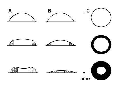
Figure 1: Sketches of models of a pinned evaporating drop. Figure A shows Popov’s model, where the deposit (shaded area) maintains its shape and modifies the geometry of the remaining evaporating drop. Figure B shows the model considered in this work. The deposit profile does not affect but passively changes with the geometry of the evaporating drop. Figure C shows the projected picture from above. The deposit (dark area) grows from the contact line toward the center of the drop.

In Popov’s picture, the deposit thickness increases monotonically toward the center of the drop until an abrupt vertical wall is formed at the end of the total drying time. The scale of the thickness is proportional to $\sqrt{\delta_{0}}$, where $\delta_{0}$ is the concentration ratio defined as the initial uniform volume concentration $C_{0}$ divided by $C_{\max}$. This $\sqrt{\delta_{0}}$-dependence near the contact line had been known before Deegan3 and is understandable heuristically. The volume of the deposit, which is proportional to the square of the thickness, multiplied by the concentration $C_{max}$, must give the total solute mass in the deposit that is proportional to $C_{0}$. However, as this dependence is largely asymptotic toward the contact line, where the time dependence is suppressed and the hydrodynamics and the deposition dynamics are largely separated, Popov’s coupled system may not be necessary to derive this result. Moreover, the complexity in Popov’s mathematical formulations may inadvertently obscure the simple and fundamental underlying physical process. Moreover, a realistic deposit clearly follows a rich profile that shows different scaling properties in different regions. Thus to interpret the deposit properties within a single asymptotic regime and with a unique $\sqrt{\delta_{0}}$ is not satisfactory.

Following the truncated transport dynamics and the simpler assumptions that the hydrodynamics and the deposition process are fully separable, Dupont Dupont1 showed by direct numerical simulation a ring-like deposit pattern with variance in areal density along the radial direction (Fig. 2 and Fig. 3). The simple mechanism thus produces a realistic deposit pattern with a pronounced maximal density near the contact line. In particular, the areal density shows a potentially analyzable characteristic profile that manifests multiple asymptotic regimes, and that could reveal robust properties of contact line deposition under general conditions.

Figure 2: Direct numerical simulation of the deposit pattern. The areal density profile is represented by variation in darkness. (Courtesy Todd Dupont)

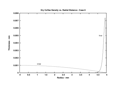
Figure 3: Areal density profile $\Sigma$ with $C_{0}/C_{\max}=0.002$, where $C_{0}=0.001$ is the initial uniform volume concentration throughout the drop. The dotted line is the initial areal density identified as the initial drop height profile multiplied by $C_{0}$. The solid line is the final areal desntity (Courtesy Todd Dupont)

In this work we re-visit Dupont’s criterion with minimal restrictions and simpler assumptions. We consider a pinned circular thin drop. In particular, we assume that the deposition process does not interfere with the hydrodynamics such as the drop geometry and flow velocity field. We consider both the uniform evaporation and the diffusion-controlled evaporation conditions, to be defined below. To interpret the deposit density, we assume that the solute particles in the deposition region, where horizontal transport is stopped, can still move vertically so that the thickness of the deposit is determined by the geometry of the drop and changes with time. The final deposit profile is thus described by its areal density when the drop dries up and the thickness becomes zero throughout the drop (Fig. 1.2B). To interpret the final deposit in terms of the areal density profile is not essential to the model, however, as we shall discuss later that the model is also valid for a deposit with finite thickness as long as the deposition does not interfere with the hydrodynamics of the evaporating drop.

We thus want to follow a reductive approach as we believe that the fundamental and robust physical properties underlying complex phenomena should be captured by a simple mathematical structure with minimal restrictions. By this approach, we want to achieve two goals. First, instead of being exhaustive in considering all the possible conditions, we want to understand the robustness of the model: among the various factors that characterize the problem what are most important in determining the key deposition properties and in yielding physically feasible and realistic deposit patterns. Second, what is the appropriate mathematical structure to describe those dominant factors, and can this mathematical structure be generalized to other physical systems.

In the rest of the work we first establish in Section 2 a one-dimensional simplification of the deposition process that we denote as “pipe models”. These models capture the important characteristics of the truncated transport dynamics. We then review the major results of the hydrodynamic properties of an evaporating drop and apply the pipe models to the evaporative deposition process with uniform evaporation in Section 3. In Section 4, we solve for the areal density profile and identify the scaling laws in different asymptotic regimes. We consider in Section 5 the deposition properties with the diffusion-controlled evaporation. In Section 6, we compare our findings with Popov’s, extending our results to interpreting the deposit in terms of the thickness profile. We then make a few comments on depinning and formation of multiple-ring patterns within the truncated transport dynamics scheme in Section 7. We discuss experimental issues and possible generalizations of the model in Section 8, and present the conclusion in Section 9. In addition, we provide an alternative derivation of the equation of motion for the shock front in Appendix.

II Pipe Models

The transport process, truncated by the maximal concentration $C_{\max}$, is naturally divided into two regions: a transport region where the concentration is smaller than $C_{\max}$, and a deposition region where there is no horizontal transport of solute particles. Solute mass is carried from the transport region to the deposition region, and the growth of the deposit is described by a characteristic moving front that separates the two regions.

We establish in this Section the so-called “pipe models” to formalize the truncated dynamics under different conditions. Although some predictions made by these models depend on pipe specifications, we find that certain important properties, such as the shock front velocity, are actually model-independent and thus generalizable. We shall show later how these universal properties may help explain the observed robustness in the general deposition phenomena.

To simplify mathematical formulations, in the following models we only treat one-dimensional case, or similarly radial symmetric case. However, we believe the key findings are readily applicable to higher dimensions.

II.1 A Uniform Pipe

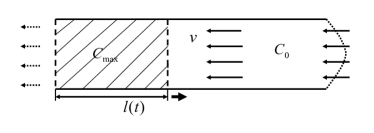
Figure 4: A uniform pipe. Solute particles with uniform volume concentration $C_{0}$ is carried at a constant velocity $v$ toward the left end of the pipe, where deposit is formed with concentration $C_{\max}>C_{0}$. $l(t)$ is the position of the moving boundary that separates the two regions with different volume concentration.

We consider a uniform pipe with simple properties (Fig. 4): incoming solute particles with constant volume concentration $C_{0}$ are transported at a constant velocity $v$ to the end of the pipe where the carrier fluid exits the pipe but the solute particles remain to form a deposit. The solute particles stop moving when their concentration exceeds $C_{\max}$, which therefore is the volume concentration of the deposit. To focus on the horizontal transport properties, we ignore the variance in velocity along the cross section of the pipe. This simplification is compatible with the basic assumptions made for the evaporative deposition problem as we shall show in the next Section.

The configuration is thus divided into two regions: a transport region with concentration $C_{0}$ and a deposition region with concentration $C_{\max}$. The boundary that separates the two regions is characterized by its position $l(t)$. Local conservation of solute mass at the boundary demands:

$$\frac{dl}{dt}=-v\frac{C_{0}}{C_{\max}-C_{0}}=-v\frac{\delta}{1-\delta},$$ (1)

where $\delta\equiv C_{0}/C_{\max}$.

Several observations immediately follow from Eq. (1). First, the boundary moves at a velocity proportional to the transport velocity $v$, and the proportional coefficient is determined by the ratio of the two volumes concentrations. Second, there must be a finite gap in volume concentration across the boundary, i.e., $\delta<1$, otherwise the velocity $dl/dt$ would diverge, which is not physical. The moving boundary is therefore a shock front that represents a discontinuity in local volume concentration profile.

It is worth noting that although the two-component simplified geometry with constant $C_{0}$ and $C_{\max}$ in the first place warrants the discontinuity and leads to the shock front, the implications of Eq. (1) are more general. If the transport process is characterized by the truncation criterion and the two-component configuration and if the boundary that separates the two regions moves with a finite velocity, there gap in concentrations across the boundary must exist as we now show.

II.2 A More Realistic Pipe: Non-Singular Case

A typical evaporating drop that we consider has a circularly symmetric geometry and an outward flow field along the radial direction. To adapt to this specific geometry, in a more realistic pipe model (Fig. 5) we introduce $h(r,t)$ as the pipe’s height profile, where $r$ is the radial distance, and allow other characteristic quantities such as the maximal volume concentration $C_{\max}$ and the transport velocity $v$ to vary both in $r$ and time $t$. In addtion, to account for the circularly symmetric geometry, our pipe must have a cross section area that varies along the radial direction as $2\pi rh(r,t)$.

This manipulation with respect to the circularly symmetric geometry may seem greatly constraint the pipe models. However, we shall show below that the major predictions made from the pipe models are actually independent of the specific form of the cross section area as long as it does not introduce significant singularities. The term $2\pi rh(r,t)$ has been introduced only to conform with the drop geometry which is not really a “pipe”.

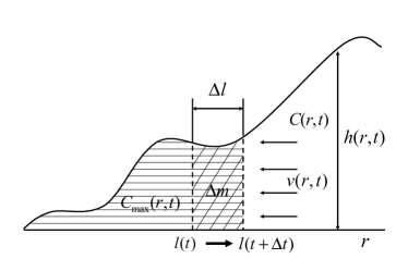
Figure 5: A realistic pipe. $r$ is the radial distance. The height profile of the pipe is $h(r,t)$. $2\pi rh(r,t)$ characterizes the cross section area, which is not shown, to account for the circularly symmetric geometry. The concentration profile $C(r,t)$ in the transport region, the flow velocity field $v(r,t)$, and the critical concentration $C_{\max}(r,t)$ are allowed to change with both the radial distance and time. $l(t)$ is the boundary that separates the deposition region and the transport region. In a small time interval $\Delta t$, $l(t)$ moves to $l(t+\Delta t)=l(t)+\Delta l$. $\Delta m$ is the change of solute mass in the transitional region.

We treat in the real pipe $h$, $C_{\max}$, and $v$ as independent specified physical quantities that have independent dynamics. This is not necessarily true in real settings such as the evaporative deposition we shall consider later, but it will allow us to derive general results and will pose not difficulties to implementing these results to specific real situations where the dynamics may couple. There are perhaps some conceptual difficulties with the functional form $C_{\max}(r,t)$. For example, because it evolves in time, what if for a position in the deposition region the $C_{\max}$ becomes smaller than the actual volume concentration in a later time? We do not consider this special case as it does not occur in the evaporative deposition problem. Nonetheless, it can be relevant in other systems with more complicated transport properties and is certainly an interesting problem for its own sake.

We again impose the truncation condition that the horizontal transport of solute mass is truncated once the local volume concentration $C(r,t)$ reaches $C_{\max}(r,t)$. As in the uniform pipe model, we consider the position $l(t)$ of the moving front that separates the deposition region and the transport region. To simplify mathematical analysis, we assume that all the introduced functions are at lease twice differentiable and that there are no singularities. We shall however discuss effects of discontinuities and other singularities later.

In the deposition region there is no horizontal transport of solute mass, and local conservation of mass requires $C(r,t)h(r,t)$ to be time-independent. In the transport region, solute mass satisfies the equation of continuity

$$\frac{\partial}{\partial t}\left(Chr\right)+\frac{\partial}{\partial r}\left(vChr\right)=0.$$ (2)

As shown in Fig. 5, during the time interval $\Delta t$ the shock front moves from $l(t)$ to $l(t+\Delta t)=l(t)+\Delta l$. To be consistent with the later-introduced context of an evaporating drop, we choose $\Delta l<0$. $l(t)$ thus decreases in time and moves toward the right end of the pipe.

We consider the change of solute mass $\Delta m$ in the transitional region $\left[l(t)+\Delta l,l(t)\right]$:

$$\Delta m =\Delta m_{1}$$

$$=\int_{t}^{t+\Delta t}2\pi l(\tau)$$

$$\times\left[C_{\max}(l\left(\tau\right),\tau)h(l\left(\tau\right),\tau)-C(l\left(\tau\right),t)h(l\left(\tau\right),t)\right]$$

$$\times\left(-\frac{dl}{d\tau}\right)d\tau,$$ (3)

i.e., $\Delta m$ is equal to the amount of solute mass in the region when it just becomes a part of the deposition region less the amount of mass in it when it is still in the transport region.

We expand $\Delta m_{1}$ up to the second order of $\Delta t$:

$$\Delta m_{1} =-2\pi l(t)$$

$$\times\left[C_{\max}(l(t),t)h(l(t),t)-C(l(t),t)(h(l(t),t)\right]\frac{dl}{dt}\Delta t$$

$$-\frac{1}{2}\frac{d}{d\tau}\{2\pi l(\tau)\frac{dl}{d\tau}$$

$$\times\left[C_{\max}(l\left(\tau\right),\tau)h(l\left(\tau\right),\tau)-C(l\left(\tau\right),t)h(l\left(\tau\right),t)\right]\left.\}\right|_{\tau=t}$$

$$\times\left(\Delta t\right)^{2}+O((\Delta t)^{3})$$

$$=-2\pi lh(C_{\max}-C)\frac{dl}{dt}\Delta t$$

$$-\pi\left[\frac{d}{dt}\left((C_{\max}-C)hl\frac{dl}{dt}\right)+\frac{\partial}{\partial t}(Ch)l\frac{dl}{dt}\right]\left(\Delta t\right)^{2}$$

$$+O((\Delta t)^{3})$$ (4)

Alternatively, $\Delta m$ is also equal to the amount of solute mass transported through $l(t+\Delta t)=l(t)+\Delta l$ from time $t$ to $t+\Delta t$:

$$\Delta m =\Delta m_{2}$$

$$=\int_{t}^{t+\Delta t}2\pi l(t+\Delta t)C(l(t+\Delta t),\tau)h\left(l(t+\Delta t),\tau\right)$$

$$\times v\left(l(t+\Delta t),\tau\right)d\tau\text{.}$$ (5)

We also expand $\Delta m_{2}$ up to the second order of $\Delta t$:

$$\Delta m_{2} =2\pi lChv\Delta t+2\pi\left[\frac{\partial}{\partial l}(lChv)\frac{dl}{dt}+\frac{1}{2}\frac{\partial}{\partial t}\left(lChv\right)\right]$$

$$\times\left(\Delta t\right)^{2}+O((\Delta t)^{3}).$$ (6)

We can now solve for $dl/dt$ given the condition $\Delta m=\Delta m_{1}=\Delta m_{2}$. If $h(l(t),t)$ is nonvanishing, the terms in the first order of $\Delta t$ must match, and thus:

$$-2\pi lh(C_{\max}-C)\frac{dl}{dt}=2\pi lChv,$$ (7)

$$\frac{dl}{dt}=-v\left(l(t),t\right)\frac{C(l(t),t)}{C_{\max}(l(t),t)-C(l(t),t)}=-v\frac{\delta}{1-\delta},$$ (8)

where $\delta=\delta(r,t)\equiv C(r,t)/C_{\max}(r,t)$.

Eq. (8) has the same form as Eq. (1) in the case of the uniform pipe though the constant quantities have been replaced here by local values of general functions dependent on position and time. The moving front is a shock front with $\delta<1$. The front velocity is proportional to the local transport velocity with opposite direction, and the proportional coefficient is determined by the local critical concentration $C_{\max}$ and the local concentration $C$ in the transport region. Eq. (8) is thus the general non-singular form of the equation of motion for the shock front in the truncated dynamics.

It also shows that the discontinuity condition $\delta<1$ is not due to the instantiations of constant $C_{0}$ and $C_{\max}$ but the requirement of finite velocity and is inherent in the truncated transport dynamics. As both concentrations are given functions, Eq. (8) imposes a specific moving boundary $l(t)$ such that a time-dependent jump in concentration across the boundary is properly maintained and the local solute mass is thus conserved.

II.3 A More Realistic Pipe: Singular Case

If the local height profile $h(l(t),t)$ is zero, the first order term in $\Delta t$ vanishes for both $\Delta m_{1}$ and $\Delta m_{2}$, and the second order terms in $\Delta t$ thus must match. The condition $\Delta m=\Delta m_{1}=\Delta m_{2}$ requires:

$$\left[\frac{d}{dt}\left((C_{\max}-C)hl\frac{dl}{dt}\right)+\frac{\partial}{\partial t}(Ch)l\frac{dl}{dt}\right]$$ (9)

$$= -2\left[\frac{\partial}{\partial l}(lChv)\frac{dl}{dt}+\frac{1}{2}\frac{\partial}{\partial t}\left(lChv\right)\right],$$

and

$$\frac{dl}{dt}=-\frac{2\left(\partial/\partial l\right)(lChv)\left(dl/dt\right)+\left(\partial/\partial t\right)(lChv)}{\left(d/dt\right)\left(\left(C_{\max}-C\right)hl\right)+l\left(\partial/\partial t\right)\left(Ch\right)}.$$ (10)

The general form Eq. (10) can be simplified under certain physical conditions. In particular, we consider the situation where $h(l(t),t)=\partial h(l(t),t)/\partial t=0$ and $\partial h/\partial l\neq 0$, which corresponds to the case when the shock front reaches a bottleneck of the pipe. In addition we assume all other quantities are nonvanishing at the bottleneck. Thus at $l(t)$

$$\frac{\partial}{\partial l}(lChv)=Cv\frac{\partial}{\partial l}(hl)\text{,}$$ (11)

$$\frac{\partial}{\partial t}\left(Ch\right)=0,$$ (12)

and

$$\frac{d}{dt}\left(\left(C_{\max}-C\right)hl\right)=\frac{\partial}{\partial t}\left(\left(C_{\max}-C\right)hl\right)$$

$$+\frac{\partial}{\partial l}\left(\left(C_{\max}-C\right)hl\right)\frac{dl}{dt}=\left(C_{\max}-C\right)\frac{dl}{dt}\frac{\partial}{\partial l}\left(hl\right).$$ (13)

Also, since $C(l(t),t)$ satisfies the equation of continuity (Eq. (2)),

$$\left(\partial/\partial t\right)(lChv)=-v^{2}C\frac{\partial}{\partial l}\left(hl\right).$$ (14)

Substituting Eqs. (11) to (14), the shock front velocity Eq. (10) is reduced to

$$\frac{dl}{dt}=-v\frac{C}{C_{\max}-C}\left(2+\frac{v}{dl/dt}\right)\text{.}$$ (15)

It can be solved for $dl/dt$:

$$\frac{dl}{dt}=-v\frac{\sqrt{\delta}}{1-\sqrt{\delta}},$$ (16)

where $\delta=\delta(l(t),t)\equiv C(l(t),t)/C_{\max}(l(t),t)$ is the local concentration ratio at $l(t)$ such that $h(l(t),t)$ vanishes.

The functional form of Eq. (16) is similar to Eq. (8) for the nonsingular case with $\delta$ replaced by $\sqrt{\delta}$. However, it is worth noting that Eq. (16) holds only at those discrete points along the pipe where the height is zero. In this sense, Eq. (16) is not a differential equation but a boundary condition or a series of boundary conditions determined by the properties of the pipe in question. We shall come back to this point in Discussion.

II.4 Truncated Transport Dynamics and the Shock Front

We have shown that the truncated dynamics in various pipe models is described by a moving shock front $l(t)$, of which the equation of motion is determined by the local values of the characteristic quantities at the front under the condition of mass conservation. We now establish the formal mathematical framework for one-dimensional truncated transport dynamics and derive the equation of motion for the characteristic shock front directly. We only treat non-singular case and omit rigorous discussion of boundary and initial conditions. In particular, we do not consider the problem how the dynamics is initiated but once it has been established what the equation of motion should be. The solution to the former depends on the boundary and initial conditions but is less relevant to applying the models to the evaporative deposition problem.

We consider a one-dimensional transport equation which imposes both the continuity condition with respect to the generalized mass $\varphi(r,t)C(r,t)$ and the truncation condition imposed on $C(r,t)$:

$$\frac{\partial}{\partial t}(\varphi(r,t)C(r,t))$$

$$+\frac{\partial}{\partial r}(v(r,t)\varphi(r,t)C(r,t)\theta(C_{\max}(r,t)-C(r,t))=0,$$ (17)

where $v(r,t)$ is the velocity field, $C_{\max}(r,t)$ is the truncation threshold, and $\theta$ is the step function defined by:

$$\theta(x)=\genfrac{\{}{.}{0.0pt}{}{1\text{, }x>0,}{0\text{, }x\leq 0.}$$ (18)

For general purposes, $\varphi\left(r,t\right)$, $C\left(r,t\right)$, and $C_{\max}\left(r,t\right)$ in Eq. (17) have no specific physical meaning attached though $\varphi(r,t)$ can be regarded as the ratio between the generalized mass and the quantity on which the truncation condition is imposed. In the case of the pipe models we have considered, $C(r,t)$ is the solute volume concentration and $\varphi\left(r,t\right)=rh(r,t)$ where $h\left(r,t\right)$ is the height profile of the pipe. For non-singular solutions, we assume $\varphi(r,t)$, $v(r,t)$, and $C_{\max}(r,t)$ are positive and at least twice differentiable.

We seek solution that admits a moving shock front $l(t)$:

$$C(r,t)=\tilde{C}(r,t)+\theta(l(t)-r)(\hat{C}(r,t)-\tilde{C}(r,t))\text{,}$$ (19)

where $\tilde{C}(r,t)$ and $\hat{C}(r,t)$ are again at least twice differentiable, $\tilde{C}(r,t)<C_{\max}(r,t)$ for $r\geq l(t)$, and $\hat{C}(l(t),t)=C_{\max}$. We show the sketch of $C(r,t)$ in Fig. 6.

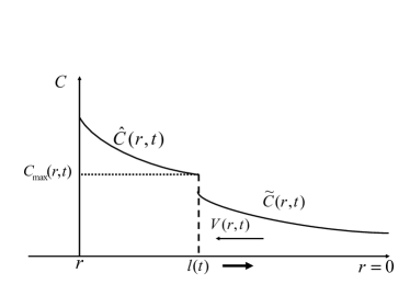
Figure 6: Sketch of the truncated dynamics solution at time $t$. The solution consists two parts: $\tilde{C}(r,t)$ in the transport region and $\hat{C}(r,t)$ in the deposition region. The two regions are separated by the shock front $l(t)$. There is a nonzero jump in $C(r,t)$ across the shock front.

Substituting Eq. (19) into Eq. (17), all singular terms must cancel each other. Thus,

$$(\varphi(\hat{C}-\tilde{C})\frac{dl}{dt}+v\varphi\tilde{C})\delta(l-r)=0,$$ (20)

and, given $\varphi(l(t),t)$ is not zero,

$$\frac{dl}{dt}=-v(r,t)\frac{\tilde{C}(l(t),t)}{C_{\max}(l(t),t)-\tilde{C}(l(t),t)}.$$ (21)

Eq. (21) is the general result of pipe models, and in the non-singular case it does not depend on $\varphi(r,t)$.

The coffee stain problem we shall discuss in the next Section corresponds to the specific case where $\varphi(r,t)=rh(r,t)$, $C_{\max}(r,t)=constant$, and $C(r,0)=C_{0}.$

III Evaporative Deposition with Uniform Evaporation

The evaporative deposition process is a special case of the pipe models above: hydrodynamics of the thin evaporating drop determines a height profile $h(r,t)$ and generates a flow velocity field $v(r,t)$; solute particles with initial uniform volume concentration $C_{0}$ are carried by the evaporation-generated flow toward the contact line, and the transport process is truncated by a maximal allowed concentration $C_{\max}$; once the volume concentration reaches $C_{\max}$, the horizontal transport is stopped and deposit forms.

The volume concentration profile of solute particles is thus divided into two regions:

Transport region. Solute particles move with the evaporation-induced flow at the same velocity and are transported toward the contact line along the radial direction. The volume concentration in this region solves the continuity equation with a finite velocity field.

Deposition region. The horizontal transport of solute particles is truncated, and only vertical movement is allowed afterward. The solute mass at each position, $i.e.$, $C(r,t)h(r,t)$ is thus conserved in time. All the solute particles eventually deposit at the position and form the areal density profile at the total drying time. We also assume that the deposition process is decoupled from the hydrodynamics of the evaporating drop, and both the height profile $h(r,t)$ and the velocity field $v(r,t$) are not affected by the deposition process.

There must be a moving shock front $l(t)$ that separates these two regions. The velocity of the front $dl/dt$ must obey the predictions made by the pipe models.

To apply the pipe models, we need to specify the height profile $h(r,t)$, the velocity field $v(r,t)$, and the solute volume concentration in the transport region. Most of these have already been explored in the existent literature Deegan3 ; Yuri3 though some exact results are not immediately available. For the sake of completeness, we shall nonetheless go through the whole derivation process from our own perspective.

III.1 Review of Evaporating Thin Drop Hydrodynamics

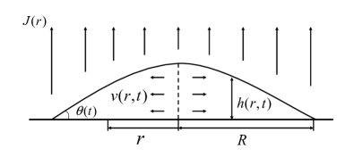
Figure 7: Sketch of an evaporating thin drop. We assume the drop is pinned during the time under consideration. The radius of the drop $R$ is thus a constant. The geometry is described by a height profile $h(r,t)$ that depends on the radial distance and time. $\theta(t)$ is the contact angle that decreases linearly in time in our approximation. $J(r)$ is the evaporation flux profile. $v(r,t)$ is the flow velocity field that also depends on the radial distance and time.

We consider a circular evaporating thin liquid drop (Fig. 7). The drop is pinned in the drying process, and the drop radius $R$ is thus a constant. The geometry of the drop is determined by the contact angle $\theta(t)$ and the height profile $h(r,t)$.

Under the assumption of slow evaporation, the quasi-equilibrium condition can be applied so that at any time the drop maintains mechanical equilibrium against the pressure difference across the liquid-air interface. The shape of the drop is thus determined by

$$\Delta p=-2H\sigma\text{,}$$ (22)

where $\Delta p=\Delta p(t)$ is the pressure difference, $H=H(t)$ is the mean curvature of the drop surface, and $\sigma$ is the surface tension. It is well known that for a circular drop the geometry that solves Eq. (22) is a spherical cap with the contact angle $\theta$ determined by:

$$\sin\theta(t)=\frac{R}{2}\frac{\Delta p(t)}{\sigma}.$$ (23)

The height profile $h(r,t)$ in this case is

$$h(r,t) =\sqrt{\frac{R^{2}}{\sin^{2}\theta(t)}-r^{2}}-R\cot\theta(t)$$

$$\approx\frac{R^{2}-r^{2}}{2R}\theta(t),\text{ \ }\theta\ll 1\text{.}$$ (24)

If the evaporation flux does not change with time, it is confirmed experimentally Deegan3 that when $\theta$ is small, the contact angle $\theta(t)$ decreases linearly with time for the most part of the drying process:

$$\theta(t)=\theta_{i}(1-\frac{t}{t_{f}}),$$ (25)

where $\theta_{i}$ is the initial contact angle and $t_{f}$ is the total drying time that depends on specific forms of evaporation profile. In what follows we shall restrict our discussion to thin drops so that the linear relation Eq. (25) is warranted.

Loss of solvent due to evaporation generates inside the drop a flow field $\mathbf{u}(r,z,t)$ with horizontal component $u_{s}(r,z,t)$, where $z$ represents the coordinate along the vertical direction. We introduce a vertically averaged velocity field

$$v(r,t)=\frac{1}{h(r,t)}\int_{0}^{h(r,t)}u_{s}(r,z,t)dz.$$ (26)

Local conservation of solvent mass then demands

$$\nabla\cdot(hv)+\frac{J(r)}{\rho}\sqrt{1+\left(\nabla h\right)^{2}}+\partial_{t}h=0,$$ (27)

where $\rho$ is the density of the solvent, and $J(r)$ is the evaporation profile defined as mass loss per unit projected area per unit time. For a thin circular drop $v(r,t)$ is along the radial direction and $\left|\nabla h\right|\ll 1$, and Eq. (27) can be integrated to solve for $v$:

$$v(r,t)=-\frac{1}{rh}\int_{0}^{r}\left(\frac{J}{\rho}+\partial_{t}h\right)rdr\text{.}$$ (28)

For uniform evaporation in which $J(r)=const.$, it can be shown that:

$$v(r,t)=\frac{1}{4}\frac{r}{t_{f}}\left(1-\frac{t}{t_{f}}\right)^{-1}.$$ (29)

where the total drying time $t_{f}$, when the whole drop dries up via evaporation, is

$$t_{f}=\frac{\rho}{\pi R^{2}J}\int_{0}^{R}2\pi h(r,0)rdr=\frac{\theta_{i}R\rho}{4J}.$$ (30)

To simplify mathematical formulations, we choose $R$ as the unit of length, $t_{f}$ as the unit of time, and $R/t_{f}$ as the unit of velocity. Thus in this model the dynamics of an evaporating drop is characterized by two dimensionless functions:

$$h(r,t)=\frac{\theta_{i}}{2}(1-r^{2})(1-t),$$ (31)

$$v(r,t)=\frac{1}{4}r(1-t)^{-1},$$ (32)

where we have used the same notations $r$ and $t$ to represent the dimensionless distance and time respectively for simplicity.

In deriving $v(r,t)$ (Eq. (32)), we have used the condition that the mass of the solvent is conserved locally (Eq. (27)), and this condition involves $h(r,t)$. Thus $v(r,t)$ and $h(r,t)$ have coupled dynamics as opposed to the general situation we considered in the real pipe models. This coupling will not pose any difficulty, however.

III.2 Solute Volume Concentration Profile

III.2.1 Concentration Profile in the Transport Region

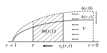
Figure 8: Sketch of the definition of $m(r,t)$. A solute particle at $r_{0}$ at time zero moves to $r$ at time $t$. $r_{0}$ as a function of $r$ and $t$ is given by Eq. (33). $m(r,t)$ is equal to the total solute mass between $r_{0}$ and $r$ (the shaded area) at time zero.

We now derive the volume concentration $C(r,t)$ in the transport region, assuming the defined height profile (Eq. (31)) and velocity field (Eq. (32)).

For radial distance $r$ and time $t$ we define $r_{0}(r,t)$ to be the initial position such that solute particles start at time zero from $r_{0}$ reach $r$ at time $t$. $r_{0}$ can be solved via integrating the velocity field (Eq. (32)):

$$r_{0}(r,t)=r(1-t)^{1/4}.$$ (33)

We next define $m(r,t)$ to be the amount of solute passing through $r$ from time zero to time $t$ (Fig. 8). Then $m(r,t)$ is equal to the total amount of solute between $r$ and $r_{0}(r,t)$ at time zero:

$$m(r,t) =2\pi\int_{r_{0}(r,t)}^{r}C_{0}h(r^{\prime},0)r^{\prime}dr^{\prime}$$

$$=\pi C_{0}\theta_{i}\left[\frac{r^{2}}{2}\left(1-\left(1-t\right)^{1/2}\right)-\frac{r^{4}}{4}t\right].$$ (34)

We consider a ring-like region between $r$ and $r+\Delta r$. At time zero the total amount of solute mass in this region is

$$m_{0}=2\pi r\Delta rh(r,0)C_{0}.$$ (35)

At time $t$, it becomes

$$m_{t}=2\pi r\Delta rh(r,t)C(r,t).$$ (36)

The change of solute mass up to time $t$ in this region should be equal to the total amount of mass moving into $r$ less the total amount of mass moving out of $r+\Delta r$,

$$\Delta m=m(r,t)-m(r+\Delta r,t).$$ (37)

Conservation of solute mass demands $m_{0}+\Delta m=m_{t}$, thus

$$C(r,t) \equiv\tilde{C}(r,t)$$

$$=\lim_{\Delta r\rightarrow 0}\left(C_{0}\frac{h(r,0)}{h(r,t)}+\frac{m(r,t)-m(r+\Delta r,t)}{2\pi r\Delta rh(r,t)}\right)$$

$$=C_{0}\frac{\left(1-t\right)^{-1/2}-r^{2}}{1-r^{2}},$$ (38)

where, in accordance with the notations in pipe models, we use $\tilde{C}(r,t)$ to denote the volume concentration in the transport region. As shown in Fig. 9, $\tilde{C}(r,t)$ increases monotonically with both $r$ and $t$.

Figure 9: The solute volume concentration profile $C(r,t)/C_{0}$ (Eq. (38)) in the transport region at $t=0.2$, $0.4$, $0.6$, and $0.8$.

The concentration profile (Eq. (38)) is a “leaking solution” in the sense that the total amount of solute mass in the transport region is not conserved, and rightly so. This can be demonstrated in an ideal evaporative deposition process such that all the solute particles are eventually carried to the contact line without truncation in volume concentration i.e., in the limit $C_{\max}\rightarrow\infty$. It is verifiable that $\tilde{C}(r,t)$ satisfies the continuity equation (Eq. (2)):

$$\frac{\partial}{\partial t}\left(\tilde{C}hr\right)+\frac{\partial}{\partial r}\left(v\tilde{C}hr\right)=0.$$ (39)

The total amount of solute mass at time $t$ in the body of the drop is

$$M(t)=\int_{0}^{1}2\pi\tilde{C}hrdr.$$ (40)

Thus the rate of change of the total solute mass is,

$$\frac{dM(t)}{dt} =\int_{0}^{1}2\pi\frac{\partial}{\partial t}(\tilde{C}hr)dr=-2\pi\int_{0}^{1}\frac{\partial}{\partial r}\left(v\tilde{C}hr\right)dr$$

$$=\left.2\pi v\tilde{C}hr\right|_{r=1}^{r=0},$$ (41)

that is, the change of the total mass is equal to the amount of mass injected into the drop (at $r=0$) less the amount of mass flowing out of the drop boundary (at $r=1$) that immediately forms deposit at the contact line. The transport process thus must be truncated with some finite threshold $C_{\max}$ so that a moving boundary is formed and the deposit grows from the contact line toward the center of the drop.

III.2.2 Concentration Profile in the Deposition Region

We are now ready to apply the pipe models. There is a shock front $l(t)$ that separates the transport region and the deposition region. The equation of motion for the shock front is given by Eq. (8) for the nonsingular case, where $\delta=C(r,t)/C_{\max}$ is the concentration ratio at the front. Substituting the height profile $h(r,t)$ (Eq. (31)), the flow velocity field (Eq. (32)), and the volume concentration profile in the transport region (Eq. (38)), the velocity $dl/dt$ is given by:

$$\frac{dl}{dt}=-v\frac{\delta}{1-\delta}=-\frac{l}{4(1-t)}\frac{1}{\frac{C_{\max}\left(1-l^{2}\right)}{C_{0}\left[(1-t)^{-1/2}-l^{2}\right]}-1}.$$ (42)

To determine $l(t)$ completely, in addition to Eq. (42), we also need to specify initial conditions. At time zero, the shock front $l(t)$ starts at the contact line: $l(0)=1$. Also, physically $dl/dt$ must have a well-define value at time zero, but naively for $t=0$ and $l(0)=1$ the right side of Eq. (42) is not well defined. The pipe models again can shed some light on this. At contact line the height is zero, and the pipe models in the singular case (Eq. (16)) require

$$\left.\frac{dl}{dt}\right|_{t=0}=-v\left(0,0\right)\frac{\sqrt{\delta_{0}}}{1-\sqrt{\delta_{0}}}=-\frac{1}{4}\frac{\sqrt{\delta_{0}}}{1-\sqrt{\delta_{0}}},\text{ }l(0)=1,$$ (43)

where $\delta_{0}=C_{0}/C_{\max}$. Eqs. (42) and (43) thus completely define the time evolution of the shock front $l(t)$.

The seeming discontinuous “jump”in $dl/dt$ from the $\sqrt{\delta_{0}}$-dependence at the contact line to $\delta$-dependence once $l$ moves away is artificial. The concentration profile in the transport region $\tilde{C}(r,t)$ (Eq. (38)) has no definite limit at the contact line for $r=1$ and $t=0$. Specific limit thus must be calculated along a definite path $r=l(t)$. The transition from $\sqrt{\delta_{0}}$ to $\delta$ is actually continuous along this path. This can be demonstrated directly (see Appendix for details), and will be further clarified later when we discuss the deposit profile properties near the contact line.

Once $l(t)$ is known, the concentration profile in the deposition region can be determined under the condition that $C(r,t)h(r,t)$ is conserved in this region. Thus for $r>l(t)$

$$C(r,t)\equiv\hat{C}(r,t)=C_{\max}\frac{h(r,l^{-1}(r))}{h(r,t)},$$ (44)

where $l^{-1}$ is the inverse function of $l$: $l^{-1}(r)$ gives the time when the shock front arrives at the position $r$. ${}^{\text{ }}$

Combining the concentration profile $\tilde{C}$ (Eq. (38)) in the transport region and the concentration profile $\hat{C}$ (Eq. (44)) in the deposition region via the moving the shock front $l(t)$, the total concentration profile is

$$C(r,t)=\tilde{C}(r,t)+\theta(r-l(t))(\hat{C}(r,t)-\tilde{C}(r,t))\text{.}$$ (45)

Alternatively the shock front velocity (Eq. (42)) and the boundary condition (Eq. (43)) can be derived directly via solute mass conservation. We show the derivation in details in Appendix.

III.3 The Shock Front

The region boundary $l(t)$ is a moving shock front, and there is a finite gap in volume concentration across the boundary.

Naively we can introduce a virtual moving front $\tilde{l}(t)$ by extrapolating the concentration profile (Eq. (38)) in the transport region with the condition $\tilde{C}(\tilde{l}(t),t)=C_{\max}$. Thus

$$\tilde{l}(t)=\left[\frac{1}{1-\delta_{0}}-\frac{\delta_{0}}{1-\delta_{0}}\left(1-t\right)^{-1/2}\right]^{1/2}\text{,}$$ (46)

where $\delta_{0}=C_{0}/C_{\max}$. $\tilde{l}(t)$ represents the location of the moving front if there were no discontinuity in volume concentration. Evidently $t\leq 1-\delta_{0}^{2}$ for Eq. (46) to be meaningful, that is, the virtual front $\tilde{l}(t)$ arrives at the center of the drop before the whole drop dries up at $t=1$.

We can also derive the equation of motion for $\tilde{l}(t)$:

$$\frac{d\tilde{l}}{dt}=-v(\tilde{l}(t),t)\frac{\delta_{0}}{\left(1-t\right)^{1/2}-\delta_{0}},$$ (47)

$$\left.\frac{d\tilde{l}}{dt}\right|_{t=0}=-\frac{1}{4}\frac{\delta_{0}}{1-\delta_{0}}.$$ (48)

Thus the virtual front moves slower than the shock front starting from the contact line.

Since for $0<t<1$ the volume concentration $C(r,t)$ (Eq. (38)) in the transport region increases with $r$ and at the shock front $C(l(t),t)<C_{\max}=C(\tilde{l}(t),t)$, thus

$$l(t)<\tilde{l}(t),$$ (49)

for $0<t<1-\delta_{0}^{2}$.

We know that $l(0)=\tilde{l}(0)=1$, and we shall prove later that $l(1-\delta_{0}^{2})=\tilde{l}(1-\delta_{0}^{2})=0$. The shock front and the virtual front thus start out from the contact line at time $t=0$ with the shock front moving faster. The virtual front then catches up, and both fronts arrive at the center of the drop at time $t=1-\delta_{0}^{2}.$ The sketches of these two fronts at time $t$ are shown in Fig. 10, and their time evolutions are shown in Fig. 11. We note that both fronts spend most of the total drying time near the contact line ($l\rightarrow 1$).

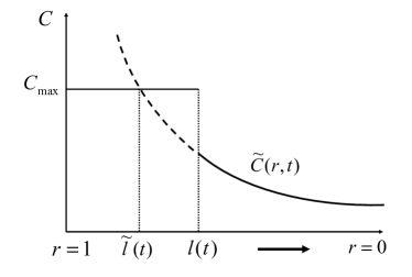
Figure 10: Sketches of the shock front and the virtual front at time $t$. The shock front is ahead of the virtual front: $l(t)<\tilde{l}(t)$. There is a nonzero jump in volume concentration across the shock front: $C_{\max}-C(l(t),t)$, with $C_{\max}=C(\tilde{l}(t),t)$.

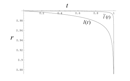
Figure 11: Time evolution of the two fronts with $\delta_{0}=0.002$. $l(t)$ and $\tilde{l}(t)$ start from the contact line ($r=1$) at time zero and arrive at the center of the drop ($r=0$) at time $t=1-\delta_{0}^{2}$.

IV Deposit Density Profile with Uniform Evaporation

IV.1 Areal Density

When a drop dries up, a ring-like stain is left with nonzero width and variation in density. The spatial profile of the deposit pattern is characterized by the areal density $\Sigma$, defined as the amount of solute mass per unit area. For a pinned circular drop without irregularities, $\Sigma$ is a function of the radial distance $r$.

Since in the deposition region there is no horizontal solute transport, at any position in this region all the solute particles distributing vertically above the position along the height of the drop will eventually deposit and form the areal density at the position. We consider a position with radial distance $r$ from the center of the drop. At time $l^{-1}(r)$ when the shock front arrives at $r$, the drop height at $r$ is $h(r,l^{-1}(r))$, and the volume concentration is exactly $C_{\max}$. Thus substituting the expression for the height profile (Eq. (31)), we find

$$\Sigma(r)=C_{\max}h(r,l^{-1}(r))=\frac{\theta_{i}C_{\max}}{2}(1-r^{2})(1-l^{-1}(r)).$$ (50)

Alternatively, via the shock front function $l(t)$ the density profile $\Sigma$ can also be expressed as a function of time

$$\Sigma(t)=\frac{\theta_{i}C_{\max}}{2}(1-l^{2}(t))(1-t),$$ (51)

representing the growth dynamics of the deposit. We shall use the same functional notation $\Sigma$ for both the areal density profile $\Sigma(r)$ and the growth dynamics $\Sigma(t)$ interchangeably without confusion.

A direct numerical solution for $l(t)$ (Eq. (42)) yields an areal density profile $\Sigma\left(r\right)$ shown in Fig. 12 and an areal density growth $\Sigma\left(t\right)$ shown in Fig. 13. The areal density profile shows that almost all the deposit occurs near the contact line with a pronounced peak followed by a steep decrease and then a long flat tail with negligible deposit. The areal density growth dynamics $\Sigma\left(t\right)$, however, shows that a significant amount of deposit occurs throughout the whole drying process with the maximal density much less pronounced in the time profile than the spatial profile. This is understandable from previous results (Fig. 11) as the shock front $l(t)$ remains near the contact line for the most of the total drying time.

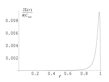
Figure 12: The areal density profile $2\Sigma(r)/(\theta_{i}C_{\max})$ from the center of the drop ($r=0$) to the contact line ($r=1$) with $\delta_{0}=0.002$, obtained by numerical solution of Eqs. (42) and (50).

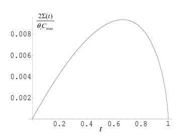
Figure 13: Areal density growth dynamics $2\Sigma(t)/(\theta_{i}C_{\max})$ with $\delta_{0}=0.002$. The time domain is essentially from $0$ to $1-\delta_{0}^{2}$.

We now study these profiles analytically via solving the solving for the shock front $l(t)$. In the small $\delta_{0}$ limit we seek the solution to Eq. (42) via asymptotic expansion. Since $0\leq t<1$, we expand $l(t)$ in terms of $t$ and thus find

$$l(t)=1-\frac{1}{4}\sqrt{\delta_{0}}t-\frac{7}{48}\sqrt{\delta_{0}}t^{2}-\frac{61}{576}\sqrt{\delta_{0}}t^{3}+O(t^{4}).$$ (52)

We look for the position $r_{m}$ and the time $t_{m}=l^{-1}(r_{m})$ for the maximal areal density near the contact line. Numerical simulations show

$$1-r_{m}^{N}=0.31...\sqrt{\delta_{0}},\ t_{m}^{N}=0.67....$$ (53)

Using first order approximation in $t$: $l(t)\approx 1-(1/4)\sqrt{\delta_{0}}t$, we find

$$1-r_{m}^{(1)}=0.125...\sqrt{\delta_{0}},\text{ \ }t_{m}^{(1)}=0.5.$$ (54)

Second and third order approximations in $t$ yield:

$$1-r_{m}^{(2)}=0.18...\sqrt{\delta_{0}},\text{ }t_{m}^{(2)}=0.55...,$$ (55)

$$1-r_{m}^{(3)}=0.22...\sqrt{\delta_{0}},\text{ }t_{m}^{(3)}=0.59....$$ (56)

It seems that different orders of approximation all show a contact line distance $1-r_{m}$ proportional to $\sqrt{\delta_{0}}$ but a maximal deposition time $t_{m}$ independent of $\delta_{0}$, and that with higher order of approximation the resulting $1-r_{m}$ and $t_{m}$ converge to the numerical results Eq. (53). We thus conjecture that, in the small $\delta_{0}$ limit, the distance between the maximal areal density and the contact line scales with $\sqrt{\delta_{0}}$, and the time at which the maximal areal density occurs is a constant portion of the total drying time. We shall confirm this conjecture later.

We also note that since throughout the drying process the majority of the deposit occurs near the contact line, we can analyze the deposit spatial profile $\Sigma\left(r\right)$ and the growth dynamics $\Sigma\left(t\right)$ separately in different asymptotic regimes.

IV.2 Asymptotic Time-Independent Deposition

We consider two cases where the time evolution of the deposition characteristics is negligible either by focusing on the depositing process in the early time regime or by controlling the experimental conditions to assure time independence.

IV.2.1 Deposition at Initial Drying Stage

The initial drying stage corresponds to the asymptotic regime $t/t_{f}\rightarrow 0$ or equivalently $t_{f}\rightarrow\infty$. Similar to the previous study Zheng1 , we consider a typical evaporative deposition scenario where there is a large pool of solution ($t_{f}\rightarrow\infty$), and we are only interested in the deposition process near the contact line ($r\rightarrow 1$) up to a time $t/t_{f}$ close to zero.

In this approximation the time dependence of all the characteristic quantities is suppressed. Thus with $t\rightarrow 0$ and $r\rightarrow 1$

$$h(r,t)\approx\frac{\theta_{i}}{2}(1-r^{2})\approx\theta_{i}\left(1-r\right),$$ (57)

$$v(r,t)\approx v(1,0)\equiv v_{0},$$ (58)

$$\delta\approx\delta_{0}=\frac{C_{0}}{C_{\max}},$$ (59)

and

$$l(t)\approx 1-\sqrt{\delta_{0}}v_{0}t.$$ (60)

The deposit profile satisfies:

$$\Sigma(r)\approx\theta_{i}C_{\max}\left(1-r\right),$$ (61)

$$\Sigma(t)\approx\theta_{i}C_{\max}\left(1-l(t)\right)\approx\theta_{i}C_{\max}\sqrt{\delta_{0}}v_{0}t.$$ (62)

The spatial profile (Eq. (61)) is trivial as it is just the time-independent drop height profile (Eq. (57)) multiplied by the maximal concentration $C_{\max}$. The growth of deposit from the contact line is linear in time with the proportional coefficient determined by the initial conditions of the drying drop.

Eq. (61) also shows, at the initial drying stage,

$$\frac{d\Sigma(r)}{dr}=-\theta_{i}C_{\max}.$$ (63)

The slope of the deposit profile near the contact line only depends on the initial contact angle and the critical concentration $C_{\max}$. We note that in this case the initial flow velocity $v_{0}$ is finite at the contact line, and this is not a general property. We shall later discuss the case of the diffusion-controlled evaporation profile where $v_{0}$ diverges, and we shall show the slope (Eq. (63)) is actually independent of the evaporation profile. Intuitively, this property is not difficult to understand. Since the time-dependence is suppressed, the slope of the areal density at the contact line should be identical/proportional to the slope of the initial drop height profile when the drying process begins, which is exactly the initial contact angle $\theta_{i}$.

IV.2.2 Deposition in Time-Independent Geometry

An evaporating drop with time-independent geometry can be achieved by replacing the evaporating fluid as illustrated in Fig. (14). Solvent is injected into the drop from below at the drop center with solvent mass $\int_{0}^{R}2\pi rJ(r)dr$ per unit time so that the total amount of solvent in the drop is constant in time. The manipulation also allows minimal perturbations to the drop shape and the flow velocity field and thus achieves a drop height profile that is approximately time-independent.

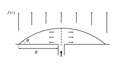
Figure 14: Sketch of a possible realization of time-independent geometry. Solvent is injected into the drop at the center from below to balance the loss due to evaporation.

The hydrodynamics in this case is thus stationary, and with uniform evaporation profile

$$h(r)=h(r,t=0)=\frac{\theta_{i}}{2}\left(1-r^{2}\right),$$ (64)

$$v(r)=v(r,t=0)=\frac{1}{4}r.$$ (65)

Using the same method (Eqs. (33), (34), and (38)), we can show that the volume concentration profile in the transport region is:

$$\tilde{C}(r,t)=C_{0}\frac{\exp\left(-t/2\right)-r^{2}\exp\left(-t\right)}{1-r^{2}},$$ (66)

where $C_{0}$ is the initial uniform volume concentration. We show the volume concentration profiles $C(r,t)/C_{0}$ at four different times in Fig. 15. As opposed to the time-dependent geometry, the concentration increases with time near the contact line but decreases close to the drop center, and there is a crossover.

Figure 15: Volume concentration profile $C(r,t)/C_{0}$ (Eq. (66)) in the time-independent geometry at $t=0.2$, $0.4$, $0.6$, and $0.8$, with $\delta_{0}=0.002$.

The spatial areal density profile is trivial:

$$\Sigma(r)=C_{\max}h(r)=\frac{\theta_{i}C_{\max}}{2}(1-r^{2}),$$ (67)

and the deposit growth dynamics is

$$\Sigma\left(t\right)=\frac{\theta_{i}C_{\max}}{2}\left(1-l^{2}(t)\right),$$ (68)

where the evolution of the shock front $l(t)$ is given by the pipe models Eq. (8).

IV.3 Density Profile in Spatial Asymptotic Regimes

IV.3.1 Near the Contact Line

We now analyze the areal density profile in spatial asymptotic regimes. We first consider the limit $l(t)\rightarrow 1$. In addition we require,

$$\delta_{0}(1-t)^{-1/2}\ll 1,$$ (69)

that is, we consider in the time regime not too late in the whole drying process as we shall show later that the shock front reaches the drop center exactly at $1-\delta_{0}^{2}$. Evidently this is satisfied for any $t<1$ for sufficiently small $\delta_{0}$.

According to the previous results for the deposit profile $\Sigma\left(r\right)$ and the growth process $\Sigma\left(t\right)$ (Fig. 12 and Fig. 13), almost all the deposit occurs throughout almost all the drying process in this asymptotic regime. Thus this regime contains most characteristics of the deposition profile. In particular, we want to look at where (the contact line distance $(1-r_{m})$) and when (time $t_{m}$) the maximal areal density occurs, and to show explicitly the scaling properties with respect to $\sqrt{\delta_{0}}$.

In this asymptotic regime Eq. (42) is reduced to

$$\frac{dl}{dt}=-\frac{\delta_{0}}{4(1-t)}\frac{\left(1-t\right)^{-1/2}-1}{1-l^{2}}.$$ (70)

With the initial condition Eq. (43), $l(t)$ can be solved for:

$$\left(1-l\left(t\right)\right)^{2}=\frac{\delta_{0}}{4}\left[2\left(1-t\right)^{-1/2}+\ln\left(1-t\right)-2\right].$$ (71)

We substitute Eq. (71) into $\Sigma(t)$ (Eq. (51)) and look for the maximal value. We find the time $t_{m}$ satisfies the following equation

$$2\ln(1-t_{m})+3\left(1-t_{m}\right)^{-1/2}-3=0.$$ (72)

Thus

$$t_{m}\approx 0.67,$$ (73)

$$r_{m}=l(t_{m})=1-0.31...\sqrt{\delta_{0}},$$ (74)

and

$$\Sigma_{m}=\Sigma\left(r_{m}\right)=0.11...\sqrt{\delta_{0}}\theta_{i}C_{\max}.$$ (75)

The maximal areal density occurs roughly at $2/3$ of the total drying time and is independent of the density ratio $\delta_{0}$ when it is small. The distance from the contact line to the maximal areal density $1-l_{m}$ and the maximal density itself, on the other hand, scale with $\sqrt{\delta_{0}}$. These results are consistent with our preliminary findings via asymptotic expansion.

We can show the scaling properties more explicitly. Near the contact line $r\rightarrow 1$ and $1-r^{2}=(1+r)(1-r)\approx 2(1-r)$ (Eq. (50)), and thus $\Sigma(r)\approx\theta_{i}C_{\max}(1-r)(1-l^{-1}(r))$. We introduce the scaled quantities

$$\tilde{\Sigma}=\frac{\Sigma}{\theta_{i}C_{\max}\sqrt{\delta_{0}}}$$ (76)

and

$$\tilde{d}=1-\tilde{r}=\frac{1-r}{\sqrt{\delta_{0}}},$$ (77)

and Eq. (51) shows

$$1-t=\frac{\tilde{\Sigma}}{\tilde{d}}.$$ (78)

Substituting Eq. (78) into Eq. (71), we find

$$\tilde{d}^{2}=\frac{1}{4}\left[2\left(\frac{\tilde{d}}{\tilde{\Sigma}}\right)^{1/2}+\ln\frac{\tilde{\Sigma}}{\tilde{d}}-2\right].$$ (79)

Eq. (79) implicitly gives the scaled universal areal density profile $\tilde{\Sigma}$ as a function of the scaled contact line distance $\tilde{d}$ (Fig. 16).

Figure 16: Scaling property of the areal density profile for small $\delta_{0}$. The scaled areal density is defined as $\tilde{\Sigma}=2\Sigma/(\theta_{i}R\sqrt{\delta_{0}})$; the scaled radial distance is defined as $\tilde{d}=\left(1-r\right)/\sqrt{\delta_{0}}$. The spectrum of curves going downward corresponding to respectively $\delta_{0}=0.1$, $0.05$, $0.01$, $0.002$, $0.001$, and $0.0005$.

Eq. (79) cannot be solved explicitly, and we instead look for the asymptotic power laws in different limits. We first consider the limit $\tilde{d}\rightarrow 0$. On the right side of Eq. (79), the term containing logarithm dominates, and thus

$$\tilde{\Sigma}\sim\tilde{d}e^{4\tilde{d}^{2}}\approx\tilde{d}.$$ (80)

The areal density increases with the contact line distance linearly. Eq. (80) is consistent with our previous findings (Eq. (61)).

We next consider the tail of the profile in the limit $\tilde{d}\rightarrow\infty$ and $\tilde{\Sigma}\rightarrow 0$. In this limit $(\tilde{d}/\tilde{\Sigma})^{1/2}$ is the dominant term, and thus

$$\tilde{\Sigma}\sim\frac{1}{4}\tilde{d}^{-3}.$$ (81)

In terms of the original varibles $\Sigma$ and $r$, Eq. (81) can be rewritten as

$$\Sigma\sim\frac{1}{4}\theta_{i}C_{\max}\frac{\delta_{0}^{2}}{\left(1-r\right)^{3}}.$$ (82)

The areal density profile is thus proportional to $\delta_{0}^{2}$ along the tail as opposed to $\sqrt{\delta_{0}}$ toward the contact line.

Similarly we can show the scaled areal density $\tilde{\Sigma}$ as a function of time $t$ explicitly:

$$\tilde{\Sigma}=\frac{1-t}{2}\left[2\left(1-t\right)^{-1/2}+\ln\left(1-t\right)-2\right]^{1/2}.$$ (83)

Eq. (83) gives the universal dynamics of deposit growth (Fig. 17).

Figure 17: Scaling property of the areal density growth dynamics for small $\delta_{0}$. The scaled areal density is defined as $\tilde{\Sigma}=2\Sigma/(\theta_{i}R\sqrt{\delta_{0}})$. The spectrum of curves going downward corresponding to respectively $\delta_{0}=0.1$, $0.05$, $0.01$, $0.002$, $0.001$, and $0.0005$.

IV.3.2 Toward the Center of the Drop

Toward the center of the drop $l\rightarrow 0$, Eq. (42) takes the form

$$\frac{dl}{dt}=-\frac{l}{4(1-t)}\frac{\delta_{0}\left(1-t\right)^{-1/2}}{1-\delta_{0}\left(1-t\right)^{-1/2}}\text{.}$$ (84)

We find in this case

$$l=A\left[1-\delta_{0}\left(1-t\right)^{-1/2}\right]^{1/2},$$ (85)

where $A$ is a constant and can not be determined without proper boundary conditions.

Thus toward the center of the drop $l(t)\propto\tilde{l}(t)$ (Eq. (46)), and as a result

$$l(1-\delta_{0}^{2})=\tilde{l}\left(1-\delta_{0}^{2}\right)=0\text{.}$$ (86)

The shock front arrives at the center of the drop at time $(1-\delta_{0}^{2})t_{f}$, and the whole horizontal transport process stops before the drop dries up.

The areal density in this case is

$$\Sigma(r)\propto\delta_{0}^{2}\frac{A^{4}(1-r^{2})}{\left(A^{2}-r^{2}\right)^{2}}\approx\delta_{0}^{2}\left[1+\left(\frac{2}{A^{2}}-1\right)r^{2}\right].$$ (87)

The density profile toward the drop center is proportional to $\delta_{0}^{2}$ in contrast with the density near the contact line where it is proportional to $\sqrt{\delta_{0}}$. This is consistent with our previous findings (Eq. (82)). For small $\delta_{0}$ majority of the deposit thus occurs near the contact line.

We also note that toward the center of the drop ($l\rightarrow 0$) it is essentially in the very final stage of the whole drying process ($t\rightarrow(1-\delta_{0}^{2})$). Practically some model assumptions may not hold at this stage. For example, the drop height profile may no long decreases linearly in time Deegan3 . However, the scaling property of $\Sigma\left(r\right)$ with respect to $\delta_{0}^{2}$ (Eq. (87)) may still be valid.

V Deposit Properties with Diffusion-controlled Evaporation

Evaporation profiles determine the hydrodynamics, such as the flow velocity field, and thus affect the deposit properties. Different evaporation profiles are achievable in experiments, and in some cases the resulting deposit patterns change dramatically with evaporation conditions Fisher1 . The uniform evaporation profile we have considered is nonsingular while the diffusion-controlled evaporation profile that has been generally assumed and studied in the literature diverges at the contact line. We shall apply the pipe models to the deposition process with the diffusion-controlled evaporation in this Section to assess the effects of evaporation condition on general deposition properties.

V.1 Hydrodynamics and Concentration Profile

We derive the hydrodynamics and solute transport dynamics of an evaporating thin drop with the same truncation concentration $C_{\max}$ but with the diffusion-controlled evaporation profile.

Assuming vapor density above the liquid-vapor interface obeys the diffusion equation and taking into account the quasi-equilibrium shape of the thin drop, the evaporation flux defined as amount of mass per unit projected area per unit time is

$$J(r)\propto(1-r^{2})^{-1/2},$$ (88)

where we still use the dimensionless representation: $r\rightarrow r/R$ and $t\rightarrow t/t_{f}$ with $0\leq r\leq 1$ and $0\leq t\leq 1$.

The height profile takes the same form as with the uniform evaporation

$$h(r,t)=\frac{\theta_{i}}{2}(1-r^{2})(1-t),$$ (89)

though physically in the dimensional domain the implicit total drying time $t_{f}$ is defined with respect to the diffusion-controlled evaporation flux as

$$t_{f}=\frac{\rho\int_{0}^{R}2\pi h(r,0)rdr}{\int_{0}^{R}2\pi J(r)rdr}.$$ (90)

Substituting Eqs. (88) and (89) into the condition of local solvent mass conservation (Eq. (28)), we solve for the velocity field

$$v(r,t)=\frac{1}{4}(1-t)^{-1}\frac{1}{r}\left[\left(1-r^{2}\right)^{-1/2}-(1-r^{2})\right].$$ (91)

The height profile (Eq. (89)) and the velocity field (Eq. (91)) thus completely determine the hydrodynamics.

To derive the solute concentration profile, we use the same method as with the uniform evaporation (Eqs. (34) and (38)). The previously defined initial position function $r_{0}\left(r,t\right)$ (Eq. (33)) and the concentration $C(r,t)$ in the transport regime have exact though complicated forms with the diffusion-controlled evaporation:

$$\left(1-r_{0}^{2}\right)^{3/2}=1-\left(1-\left(1-r^{2}\right)^{3/2}\right)\left(1-t\right)^{3/4}$$ (92)

and

$$C(r,t) =C_{0}(1-t)^{-1/4}(1-r^{2})^{-1/2}$$

$$\times\left\{1-\left[1-\left(1-r^{2}\right)^{3/2}\right](1-t)^{3/4}\right\}^{1/3}.$$ (93)

The pipe models can be applied to derive the equation of motion of the moving shock front

$$\frac{dl}{dt}=-v\frac{\delta}{1-\delta},$$ (94)

where $v(r,t)$ is given by Eq. (91), and $\delta=C/C_{\max}$ with $C(r,t)$ given by Eq. (93).

At the contact line $dl/dt\rightarrow-v(1,0)\sqrt{\delta_{0}}/(1-\sqrt{\delta_{0}})$. It is finite for the uniform evaporation, but divergent in the diffusion-controlled case (Eq. (91)). We shall show later that this divergence does not affect the deposit properties near the contact line.

As in the case of the uniform evaporation we can also introduce the virtual front $\tilde{l}(t)$ by imposing the condition $C(\tilde{l}(t),t)=C_{\max}$, where $C(r,t)$ is given by Eq. (93). The terminal time when the virtual front arrives at the center of the drop is given by the condition $C(0,t)=C_{\max}$, and we find

$$t=1-\delta_{0}^{4}.$$ (95)

Thus the whole transport process stops at $(1-\delta_{0}^{4})$ of the total drying time for the diffusion-controlled evaporation as opposed to $(1-\delta_{0}^{2})$ for the uniform evaporation.

V.2 Deposit Density Profile

For the case of the diffusion-controlled evaporation, the areal density profile $\Sigma(r)$ and the growth dynamics $\Sigma(t)$ are completely solved by Eqs. (50), (51), and (94). We show the numerical results for the density profile and the growth dynamics in Fig. 18 and Fig. 19. The corresponding results in the case of the uniform evaporation are also shown for comparison.

Figure 18: Deposition profiles with $\delta_{0}=0.002$. The solid line corresponds to the case of the uniform evaporation. The dotted line corresponding to the case of the diffusion-controlled evaporation.

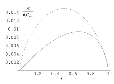
Figure 19: Deposition growth dynamics with $\delta_{0}=0.002$. The solid line corresponding to the case of the uniform evaporation. The dotted line corresponding to the case of the diffusion-controlled evaporation.

The diffusion-controlled evaporation thus yields more pronounced deposit density near the contact line as the singular flow field (Eq. (91)) carries more solute particles toward the contact line at early time. For the areal density profile, two asymptotic regimes can again be identified as detailed later, with majority of the deposit occurs near the contact line. For the deposit growth dynamics, however, significant amount of deposit occurs throughout the whole drying process. Thus the two different evaporation conditions lead to density profiles and growth dynamics with qualitatively similar properties.

We now study the asymptotic regimes quantitatively. Toward the contact line, we consider the limit $r\rightarrow 1$ and $\delta\rightarrow\delta_{0}\ll 1$. The equation of motion for the shock front (Eq. (94)) reduces to

$$\frac{dl}{dt}=-\frac{\delta_{0}}{8(1-t)}\frac{1}{1-l}\left(1-t\right)^{-1/4}\left(1-\left(1-t\right)^{3/4}\right)^{1/3}.$$ (96)

With the condition $l(0)=1$, Eq. (96) admits a solution of the form:

$$\left(1-l\right)^{2}=\frac{\delta_{0}}{3}\int_{(1-t)^{3/4}}^{1}(1-x)^{1/3}x^{-4/3}dx.$$ (97)

Using the scaled density profile $\tilde{\Sigma}$ (Eq. (76)) and the scaled contact line distance $\tilde{d}$ (Eq. (77)), we can rewrite Eq. (97) as

$$\tilde{d}^{2}=\frac{1}{3}\int_{\left(\tilde{\Sigma}/\tilde{d}\right)^{3/4}}^{1}(1-x)^{1/3}x^{-4/3}dx,$$ (98)

and

$$\left(\frac{\tilde{\Sigma}}{1-t}\right)^{2}=\frac{1}{3}\int_{(1-t)^{3/4}}^{1}(1-x)^{1/3}x^{-4/3}dx.$$ (99)

Eqs. (98) and (99) thus give the universal density profile and growth dynamics in the limit $\delta_{0}\rightarrow 0$.

Subjecting the growth dynamics Eq. (99) to the condition of vanishing derivative with respect to time, we find that $t_{m}$, when the maximal areal density occurs, satisfies the equation:

$$\frac{2(1-t_{m})}{3}\int_{(1-t_{m})^{3/4}}^{1}(1-x)^{1/3}x^{-4/3}dx$$

$$-\frac{1}{4}(1-(1-t_{m})^{3/4})^{1/3}(1-t_{m})^{3/4}=0.$$ (100)

Eq. (100) can be solved numerically, and thus

$$t_{m}=0.50...$$ (101)

It is worth noting that $t_{m}$ is not exactly $0.5$, and Eq. (100) is not exactly symmetric about $t_{m}$ though the reverse might seem true from Fig. 19.

Substituting $t_{m}$ into the shock front solution Eq. (97) and the areal density profile Eq. (50), we find the contact line distance for the maximal density

$$1-r_{m}=0.33...\sqrt{\delta_{0}},$$ (102)

and the maximal areal density

$$\Sigma_{m}=0.17...\sqrt{\delta_{0}}\theta_{i}C_{\max}\text{.}$$ (103)

We also look for the power law governing the tail decay of the scaled universal profile $\tilde{\Sigma}$. In the limit $\tilde{d}\rightarrow\infty$, the right side of Eq. (98) must diverge and the integrand must be asymptotically dominated by $x^{-4/3}$ in the lower limit $(\tilde{\Sigma}/\tilde{d})^{3/4}\rightarrow 0$. Thus Eq. (98) reduces to the following power law:

$$\tilde{\Sigma}\sim\tilde{d}^{-7},$$ (104)

and in terms of the original variables $\Sigma$ and $r$

$$\Sigma\sim\theta_{i}C_{\max}\frac{\delta_{0}^{4}}{\left(1-r\right)^{7}}.$$ (105)

In comparison with the uniform evaporation profile, a more pronounced maximal areal density occurs earlier at about $1/2$ of the total drying time as opposed to $2/3$ of the total drying time, but at about the same distance from the contact line. The areal density profile near the contact line still obeys the $\sqrt{\delta_{0}}$-scaling law. Away from the contact line, however, the density profile decays much faster and is proportional to $\delta_{0}^{4}$ as opposed to $\delta_{0}^{2}$ for the uniform evaporation.

We are for the first time able to derive the power-law decay (Eqs. (82) and (105)) of the deposition profile toward the center of the drop. Although we have based the derivation on specific deposition mechanism and simple conditions, these asymptotic results reflect the behavior of the shock front at a late time, and thus may reveal general properties of the evaporative deposition phenomena. We shall come back to this point later in Discussion.

VI Comparison with Popov’s Model

As mentioned in Introduction, Popov Yuri3 applied the same truncation criterion by Dupont to a similar problem with different conditions and assumptions. Unlike our analysis so far, Popov studied the solute transport process with diffusion-controlled evaporation and analyzed the final deposit pattern in terms of the thickness profile. These differences are not essential, however, as we shall discuss below. Most importantly Popov assumed that the deposition region interferes with the transport region and the hydrodynamics of the evaporating drop. In particular, the formed deposit with finite thickness alters the boundary conditions under which the drop shape is determined. In Popov’s model the drop shape is thus truncated by the deposit: the drop shape in the deposition region is identical to the thickness profile of the formed deposit while in the transport region it is described by a spherical cap elevated by the amount of deposit thickness at the boundary. As a result, the velocity field, determined by conservation of the solvent mass, also depends on the deposit thickness, and the deposition process thus couples with the transport process. This assumption, though more realistic, makes the underlying mathematical structure more complicated, and a complete solution is not available. Popov showed the asymptotic deposition properties near the contact line under these assumptions. We shall compare our findings with these results to shed some light on the model robustness.

VI.1 Thickness Profile

We have described the final deposit pattern in terms of the areal density profile. To implement this description, we assume that in the deposition region, where horizontal transport is stopped, solute particles can still move vertically so that the deposit thickness decreases along with the drop height profile and eventually reaches zero. At the same time, the volume concentration diverges and is replaced by the areal density profile. This zero-thickness assumption is not essential as long as the deposition region does not interfere with the geometry and hence the hydrodynamics of the evaporating drop. Alternatively we can interpret the final deposit in terms of the thickness profile. In this description solute particles cannot move vertically either once the volume concentration reaches $C_{\max}$. Thus the thickness profile of the deposition region does not change with time once formed and the volume concentration is uniformly $C_{\max}$ throughout the deposit. The evaporating drop, on the other hand, still maintains its spherical-cap equilibrium shape with height profile decreasing in time, and the evaporation flux and the flow velocity field are not affected by the deposit. Essentially these two descriptions correspond to two different deposit dynamics in the deposit region during the drying process: in the areal density description, the deposit height profile is identical to the drop height profile $h(r,t)$ and vanishes at the total drying time; in the thickness description, the density profile is characterized by the function $h(r,l^{-1}(r))$ and is independent of time. We sketch these two descriptions in Fig. 20.

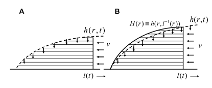
Figure 20: Sketch of the two descriptions. The shaded area is the deposition region. The dotted line outlines the height profile of the evaporating drop that decreases in time. The solid line shows the thickness profile of the formed deposit. A: description in terms of the areal density profile where solute particles move vertically in the deposition region and the height profile of the region follows that of the drop; B: description in terms of the thickness profile where the thickness of the deposit is described by $H(r)$.

The two mathematical formulations for the deposit profile are essentially the same as the solute mass across the thickness at each position in the deposition region is constant without horizontal transportation. The areal density profile is given by $\Sigma\left(r\right)=C_{\max}h(r,l^{-1}\left(r\right))$ (Eq. (50)), and thus

$$H\left(r\right)\equiv\frac{\Sigma\left(r\right)}{C_{\max}}=h(r,l^{-1}(r))$$ (106)

is the corresponding thickness profile. Since $H(r)$ is proportional to $\Sigma(r)$ with the constant coefficient $C_{\max}$, our previous findings for $\Sigma\left(r\right)$ are readily applicable to $H\left(r\right)$ with almost no modifications.

The mathematical equivalence is based on the same underlying physical assumption that the deposition process does not interfere with the transport process and should be distinguished from Popov’s model. This assumption may seem even farther from reality in the thickness description as finite accumulation of the deposit almost certainly alters the velocity field and hence the transport process. However, as we shall show later deposition properties are actually independent of the specific physical assumptions in some asymptotic regimes.

VI.2 Asymptotic Deposit Properties

We first consider, in the limit $t\rightarrow 0$, $r\rightarrow 1$, the slope of the deposit thickness profile $dH/dr$. With $\Sigma$ given by Eq. (50),

$$\frac{d\Sigma}{dr} =-r\theta_{i}C_{\max}\left(1-l^{-1}(r)\right)-\frac{1}{2}\theta_{i}C_{\max}(1-r^{2})\frac{dl^{-1}(r)}{dr}$$

$$=-\theta_{i}C_{\max}-\frac{1}{2}\theta_{i}C_{\max}(1-r^{2})\left(\frac{dl}{dt}\right)^{-1}.$$ (107)

In the limit the second term on the right side of Eq. (107) is proportional to $h(1,0)/v(1,0)$ at the contact line and vanishes. Thus near the contact line in the early drying stage $d\Sigma/dr\rightarrow-$ $\theta_{i}C_{\max}$ and thus $dH/dr\rightarrow-\theta_{i}$, which is independent of the evaporation profile (compared with Eq. (63)).

We next consider the growth dynamics of the deposit thickness $H(t)\equiv\Sigma\left(t\right)/C_{\max}$ at the early drying stage. Since $H\left(r\right)$ as shown above is proportional to $\left(1-r\right)$ in this limit, thus

$$H(t)=H\left(r\right)\rightarrow\theta_{i}\left(1-l\left(t\right)\right).$$ (108)

For the uniform evaporation, it is given by Eq. (62). For the diffusion-controlled evaporation we note that near the contact line $dl/dt\rightarrow-\sqrt{\delta_{0}}v(l,t)$, and thus in this limit

$$1-l(t)\approx\sqrt{\delta_{0}}\left(1-r_{0}(1,t)\right),$$ (109)

where $r_{0}\left(r,t\right)$ is the initial position function (Eq. (92)).  With $r=1$, $t\rightarrow 0$, and $r_{0}\rightarrow 1$, the leading order term of $H(r)$ (Eq. (92)) is

$$H\left(t\right)\approx\sqrt{\delta_{0}}\theta_{i}\frac{\left(3t\right)^{2/3}}{2^{7/3}},$$ (110)

using $\left(1-r_{0}^{2}\right)\approx 2\left(1-r_{0}\right)$ and $1-r_{0}\approx(1/2)(1-(1-t)^{3/4})^{2/3}\approx(3t)^{2/3}/{2^{7/3}}$.

The asymptotic form Eq. (110) is exactly the same as the result derived in Popov’s case Yuri3 . This sameness is not a surprise. In solving the system of coupled equations, Popov argued that the solutions can be expanded in terms of $\sqrt{\delta_{0}}$. In the lowest order the equations decouple, and it physically corresponds to the condition that the deposition process and the hydrodynamics are separated. Thus our result Eq. (110) (as well as the assumption of decoupling) is the lowest order approximation to Popov’s findings near the contact line at the early drying stage.

The later drying stage when $t$ is large, however, was not well defined in Popov’s results. Popov suggested that, in the limit $\delta_{0}\rightarrow 0$, the thickness profile $H(r)$ monotonically increases with $t$ and eventually approaches a limit $H_{m}$ that is proportional to $\sqrt{\delta_{0}}$ toward the end of the drying process ($1-t\ll 1$). The thickness profile thus ends abruptly with a “vertical wall” at its inner side. Although our finding of the maximal thickness $H_{m}\equiv\Sigma_{m}/C_{\max}$ has the same $\sqrt{\delta_{0}}$-dependence (Eqs. (75) and (103)), the universal properties of the profile show that $H_{m}$ is formed at about $2/3$ (uniform evaporation) or $1/2$ (diffusion-controlled evaporation) of the total drying time and the thickness decreases continuously afterward following a power-law decay (Eqs. (82) and (105)). Furthermore, our results clearly show two different asymptotic regimes and the thickness profile is instead proportional to $\delta_{0}^{2}$ (uniform evaporation) or $\delta_{0}^{4}$ (diffusion-controlled evaporation) in the late drying stage toward to center of the drop. Neither the $\sqrt{\delta_{0}}$-universality of the thickness profile near the contact line nor the power-law decay toward the center of the drop was apparent in Popov’s findings.

The coupled system Popov studied is thus fully reducible to the simpler conditions we have assumed in the small $\delta_{0}$ limit. This coupling between the deposition and the hydrodynamics is further resolved near the contact line in the limit $r\rightarrow 1$ (this is consistent with the $\sqrt{\delta_{0}}$-scaling property of $(1-r)$). It is thus fairly reasonable to argue that the evaporative deposition phenomenon is robust against specific assumptions and conditions in this asymptotic regime. Additionally as we have shown that the temporal properties of the process are actually $\delta_{0}$-independent, by assuming the decoupling we are able to specify a universal time scale when the maximal deposit thickness forms and to extend the truncated deposition model to a separate new asymptotic regime toward the center of the drop.

Furthermore, it is worth pointing out that even Popov’s treatment in Yuri3 only partly addresses the coupling between the formed deposit and hydrodynamics, and a few important dynamical aspects are still missing. First, the deposit-dependent drop shape alters the boundary conditions under which the evaporation flux is determined and hence further changes the velocity field. Second, the velocity field in the deposition region should be certainly affected by the deposit. If the deposit takes up a nonzero fraction of the volume, a given evaporation flux will take the same amount of available solvent per unit time but with a larger effective volume in the deposition region, and a larger velocity is required to replenish this solvent. However, our findings suggest that by controlling the initial concentration ration $\delta_{0}$ all these couplings might be effectively suppressed near the contact line at the early drying stage and may not alter the deposition properties. Also, further considerations of these couplings are important for experimentally testing the model. We shall discuss this issue later.

VII Comments on Depinning and Multiple-Ring Patterns

In the evaporative deposition model, we have identified one key deposition mechanism: horizontal transport of solute particles truncated by maximal allowed volume concentration. This truncated dynamics is robust in the sense that it admits a solution with a moving shock front that has a definite functional form independent of the dynamical characteristics of the problem. The shock front velocity only depends on local values of the flow velocity, the pipe geometry, and the volume concentration in the transport region. Furthermore, the truncated transport mechanism leads to a characteristic deposit profile near the contact line that is independent of evaporation conditions and dynamical couplings in the early drying stage.

Although practically evaporative deposition phenomena are rich and there must be many complex underlying mechanisms, we now discuss how the truncated transport dynamics, as a single deposition mechanism, might yield general deposit profiles under some typical and controllable conditions.

VII.1 Depinning Configuration

For an actual evaporative deposition process Deegan3 , in the late drying stage the contact line of a evaporating drop can depin and retreat toward the drop center before it is pinned again, and the deposition process is restored at the newly-formed contact line. The slip-stick process may occur many times before the drop tries up and thus yield a multiple-ring pattern Stone2 ; Jia1 ; Xu1 ; Hong1 .

There is still no consensus on a general depinning mechanism, which may not exist after all. A conventional explanation Deegan3 ; Yuri3 ; Nonomura1 calls for the Young-Dupre equation at the contact line Witten1 : $\gamma_{lv}\cos\theta+\gamma_{sl}-\gamma_{vs}=0$, where $\theta$ is the contact angle, and $\gamma_{lv}$, $\gamma_{sl}$, and $\gamma_{vs}$ are the surface tensions at liquid-vapor, solid-liquid, and vapor-solid interfaces. The horizontal component of the surface tension along the liquid-vapor interface at the contact line $\gamma_{lv}\cos\theta$ acts as the depinning force that increases as the drop progressively flattens toward the late drying stage. $\gamma_{sl}$ also contributes to the depinning force, but it primarily depends on the local deposition and is less affected by the geometry.

Admittedly this explanation can be problematic in that it predicts an extremely narrow range of deposit thickness and drop configurations when the maximal horizontal depinning force is achieved and the contact line depins. In reality, however, the depinning occurs over a wide range of configurations. To account for this smooth change, the conventional explanation thus must be complemented by other mechanisms that are still lacking. We shall in the following consider within the framework of the conventional theory and cautiously keep its limitations in mind.

The depinning phenomenon thus clearly involves the coupling between the deposition process and the hydrodynamics of the evaporating drop: the drop geometry and therefore the contact angle $\theta$ must be determined from the boundary conditions defined by the formed deposit pattern to account for the change of the depinning force (Fig. 1.2A). To continue our discussion of depinning within the model established in the previous Sections, we must adopt the view that our results based on the assumption of decoupling can be applied to the coupling system in the lowest order of $\delta_{0}$, and we also must interpret the deposit pattern in terms of the thickness profile $H$.

Deegan showed experimentally Deegan3 that the depinning time $t_{d}$ is about $0.4$ to $0.8$ (in the unit that the total drying time $t_{f}=1$) and it depends on the initial volume concentration $\delta_{0}$ (from $0.001$ to $0.01$). We have found that in the small $\delta_{0}$ limit, the maximal areal density and hence the maximal deposit thickness occurs at time $t_{m}\approx 0.67$ (Eq. (73)) for the uniform evaporation and $0.50$ (Eq. (101)) for the diffusion-controlled evaporation. Our $t_{m}$ thus falls in the range of the depinning time found in experiments. Geometrically the maximal deposit thickness occurs when the contact angle $\theta$ at the rim of the deposit becomes zero and the depinning force $\gamma_{lv}\cos\theta$ achieves its maximal value.

To derive $t_{m}$ formally, we note that $H(t)=\Sigma\left(t\right)/C_{\max}=(\theta_{i}/2)h(l(t),t)$ (Eq. (51)), and thus the condition $dH/dt=0$ demands

$$\frac{\partial h}{\partial t}+\frac{\partial h}{\partial r}\frac{dl}{dt}=0.$$ (111)

Eq. (111) does not depend on model assumptions as $h(r,t)$ can be the drop height profile under any conditions. In particular, $h(r,t)$ can be the solution to the drop geometry coupled with the deposition process. $dl/dt$, on the other hand, must be given by the pipe model results Eq. (8). Eq. (111) gives the general condition and scheme to solve for $t_{m}$ when the maximal thickness occur within the truncated transport model.

However, $t_{m}$ is only an approximation for the depinning time $t_{d}$. The depinning may occur once the contact angle is small enough but not necessarily zero, and as a result $t_{d}\leq t_{m}$. More importantly, our finding of $t_{m}$, as opposed to Deegan’s results, does not depend on the initial concentration (Fig. 17) when $\delta_{0}$ is small. This dependence may be included in the higher order solution in $\delta_{0}$ when the coupling between deposition and geometry is considered. The dependence can also reflect the dependence of $\gamma_{sl}$ on $\delta_{0}$. Nevertheless our finding of $t_{m}$ within the truncated transport model is consistent with empirical evidence and may be instructive for further studies.

Also, for the complicated depinning process the above explanation based on Deegan’s experimental results is not universal. Other mechanisms, such as the tension within the formed deposit Gennes2 , the kinetic processes controlled by the viscous stress in the drop, or the diffusion relaxation in air, may affect the depinning under certain conditions and thus lead to different interpretation of the depinning time.

VII.2 Formation of Multiple-Ring Patterns

The depinning process can lead to multiple-ring deposit patterns: the retreating contact line is rested at a nearer position toward the drop center and the deposition process continues at this newly formed contact line. In Refs. Adachi1 and Nonomura1 , a slip-stick theory was established, where the Young-Dupre condition was incorporated into the equation of motion for the contact line. As a result, the contact line was found to follow a sinusoidal motion, and this led to a very dense multiple-ring pattern. The authors in Refs. Stone2 and Xu1 considered controllable multiple-ring formation in nonconventional geometries. Some of these empirical evidence may need explanations that are different from Deegan’s framework Deegan3 .

Following our discussion on the depinning process, we consider an ideal model for the multiple-ring formation. For the diffusion-controlled evaporation, we identify the depinning time $t_{d}=t_{m}\approx 1/2$ ($2/3$ for the uniform evaporation), i.e., the contact line is released when the contact angle becomes zero. The width of the deposit ring is identified as $\left(1-l_{m}\right)$ (Eq. (74)). The thickness is represented by the maximal thickness $H_{m}=\Sigma_{m}/C_{\max}$ (Eq. (75)).

The newly pinned position $R^{\prime}$ can be determined by considering the change of the solvent volume. Initially for small contact angle $\theta_{i}$, the total volume of the drop is

$$V\approx\frac{\pi}{4}R^{3}\theta_{i}\text{.}$$ (112)

We assume the contact line moves fast enough to the new position so that the time it takes can be ignored compare to the time when it is pinned. Since the evaporation flux is stationary, the volume of the drop when the contact line is pinned again is thus $V(1-t_{d})\approx V/2$ ($V/3$ for the uniform evaporation). For slow evaporation, the newly pinned drop must still maintain a spherical cap geometry. The contact angle at the new contact line must still be approximately $\theta_{i}$ since it is determined by the Young-Dupre condition. Thus we find

$$R^{\prime}\approx\left(\frac{1}{2}\right)^{1/3}R\approx 0.8R\text{,}$$ (113)

and $R^{\prime}\approx 0.7R$ for the uniform evaporation.

We next consider the width and the thickness of the new deposit ring. The deposition process via truncated transport is restored at the newly formed contact line, and the deposit growth there must follow what we have found at the initial contact line. Since $R(1-r_{m})\propto R\sqrt{\delta_{0}}$ (Eq. (74)) and $H_{m}\propto R\sqrt{\delta_{0}}$ (Eq. (75)) (we now have added $R$ to the dimensionless expressions), for the new ring we replace $R$ with $R^{\prime}$ and replace $\delta_{0}$ with concentration ratio at the new contact line: $\delta_{0}^{\prime}\approx C(R^{\prime},t_{d})/C_{\max}\approx 2.2\delta_{0}$ in the case of the diffusion-controlled evaporation profile (Eq. (38)) ($2.4\delta_{0}$ for the uniform evaporation). Thus the width $R^{\prime}(1-r_{m}^{\prime})$ and the thickness $H_{m}^{\prime}$ of the new ring satisfies:

$$R^{\prime}(1-r_{m}^{\prime})\approx 1.1R(1-r_{m}),$$ (114)

$$H_{m}^{\prime}\approx 1.1H_{m}\text{.}$$ (115)

For uniform evaporation, they are $1.2R(1-r_{m})$ and $1.2H_{m}$ respectively. The thickness and height of the secondary ring are thus comparable to those of the initial ring.

There can be further depinning events in this ideal model. Following the above reasoning, for the $n$-th order ring (the initial ring is the zeroth order with the radius $R$) toward the drop center, the time it starts to form (the depinning time of the $\left(n-1\right)$-th ring), the radius, and the concentration ratio are

$$t_{d}^{\left(n-1\right)}\approx\frac{1}{2}\sum_{k=0}^{n-1}\left(\frac{1}{2}\right)^{k}=1-\frac{1}{2^{n}}\text{,}$$ (116)

$$R^{(n)}\approx\left(\frac{1}{2}\right)^{n/3}R\text{,}$$ (117)

and

$$\delta_{0}^{(n)}\approx\frac{C(R^{(n)},t_{d}^{(n-1)})}{C_{\max}}=\frac{2^{7n/6}-1}{2^{2n/3}-1}\delta_{0}\text{.}$$ (118)

Thus the width and the thickness of the $n$-th ring are

$$R^{(n)}(1-r_{m}^{(n)})\approx\left(\frac{1}{2}\right)^{n/2}\left(\frac{2^{7n/6}-1}{2^{2n/3}-1}\right)^{1/2}R(1-r_{m})\text{,}$$ (119)

$$H_{m}^{(n)}\approx\left(\frac{1}{2}\right)^{n/2}\left(\frac{2^{7n/6}-1}{2^{2n/3}-1}\right)^{1/2}H_{m}\text{.}$$ (120)

The results for the uniform evaporation can be derived similarly.

Empirically deposit patterns with major multiple rings were observed by Deegan Deegan3 . In Fig. 21, for two initial concentrations (a) 0.01 and (d) 0.00063 there are major higher-order rings up to the third order with width and thickness comparable to the zeroth order ring at the initial contact line. Our above analysis in the highly ideal case is at least consistent with the observed pictures. For the other two initial concentrations (cases (b) and (c)), however, major higher-order rings are not observed.

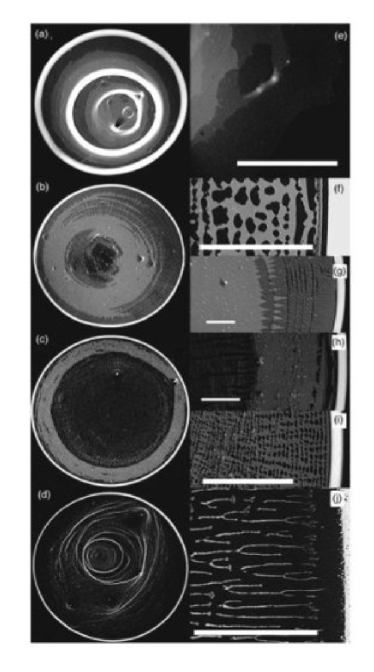
Figure 21: Photographs of the deposit patterns in Deegan’s experiment Deegan3 . The left column shows the entire deposit for initial volumn concentration (a) 0.01, (b) 0.0025, (c) 0.0013, (d) 0.00063. The right column shows the close-ups. (Courtesy Robert Deegan)

Between the major rings Deegan’s results clearly show some fine complex patterns. In our ideal case, these fine patterns are formed by the solute particles in the region where the depinned contact line sweeps through between two pinning events. Thus they must be formed within a much smaller time scale compared to the major ring formation according to our assumptions. Formation of those fine structures, as a result, may not be explained within the framework of the truncated transport dynamics considered in this work. Instead, other mechanisms, such as the dynamics and instabilities of the dewetting of thin films Gennes3 ; Ohara1 ; Nakanisi1 where capillary forces are important and long-range interactions between solute particles are relevant Brenner1 ; Nierop1 , are needed to account for the observed patterns in those regimes.

VIII Discussion

VIII.1 Experimental Aspects of the Model

Experimental tests involve two aspects of the model. First, Dupont model is based on some assumptions and conditions that require specific experimental design and realization. Second, testability depends on the major predictions made by the model. We shall discuss these in turn.

The decoupling between the deposition process and the transport process is the major assumption. This ideal case can be approximated under certain experimental conditions.

One of the key parameters in Dupont model is the allowed maximal concentration $C_{\max}$. $C_{\max}$ should depend on the size of the solute particles, interactions between the solute, the solvent, and the substrate. $C_{\max}$ could be also affected by other dynamic factors, such as the flow velocity. Empirical data for $C_{\max}$ is limited, but naively $C_{\max}$ can be deduced from the initial volume concentration by measuring the volume of the major deposit rings and comparing it with the initial volume of the entire drop.

The assumption of decoupling requires $C_{max}$ be small. Any solid particles must become immobilized if their concentration is high enough. For simply shaped particles, the immobilization occurs at volume fractions of order unity. However, the immobilizing volume fraction can be much smaller than unity if the solute consists of tenuous objects like polymers, especially those that form a physical gel Witten1 . Many organic solutes such as food may well be of this sort, and seem most appropriate for the model.

Another aspect of the coupling is that the formed deposit may alter the drop geometry which in turn changes the evaporation flux and its generated flow field. One way to bypass this obstacle is to realize the uniform evaporation profile as sketched in Zheng1 . The uniform evaporation, unlike the diffusion-controlled case, is maintained by the peripheral environment but not the drop itself. The coupling due to change of the evaporation condition is thus effectively avoided.

Furthermore, some kinetic effects such as Marangoni flows and viscous stress may deviate from the Dupont model assumptions and the fundamental lubrication approximation. Convective Marangoni flows can be avoided by maintaining uniform experimental conditions such as the temperature and by reducing the thermal effect due to evaporation. Viscous stress effect can be also reduced by slowing the evaporation. Thus by making the environment nearly saturated with the solvent vapor, these kinetic effects can be made arbitrarily small.

Our work allows one to compare the predictions of the Dupont model with experiment quantitatively in several new ways. Our main prediction is about the normal density profile. There are three aspects that might be tested: the leading edge, the time and position of the maximal deposition, and the trailing edge.

The leading edge prediction states that the areal density should increase linearly with distance from the contact line, and that the slope is proportional to the square root of the initial concentration ratio. This prediction is identical to Popov’s results and is therefore not a particular test of Dupont model. The maximal deposition time, on the other hand, is a strong test and comes out very clearly from our findings.

The power-law decay of the areal density at the trailing edge is also a strong test. On the qualitative level, this decay appears consistent with some experiments but not others. Often with colloidal solutes, such as in some of Deegan’s experiments, one sees a sharp inner edge with no apparent decay at all. This is not a surprise. As noted above, Dupont model is not completely applicable with compact solid solutes. Moreover, a continuum model such as Dupont’s should not work completely when the solute particles have a size comparable to the drop thickness $h$.For non-colloidal solutes, there should be a decay that is consistent with our predictions for $C_{max}$ small enough.

For quantitative prediction, one should measure the density or thickness of the deposit as a function of distance as well as drying time. The function of distance can be straightforwardly measured for the dried deposit. The function of drying time can be measured by monitoring and recording the whole drying process. The shock front velocity might be also measured this way.

VIII.2 Generalizations of the Model

We have not considered any kinetic effects such as visous stress and diffusion in the work. These effects will modify the physical assumptions and mathematical formulations. For example, we implement a step function to model the deposition condition with respect to the threshold concentration $C_{max}$. Horizontal diffusion and forces between various media may smooth the transition to immobility. Mathematically this effect can be modelled by replacing the step function with a weakly convergent series, and the truncated transport equation thus becomes nonsingular. This is an interesting mathematical problem. Physically we want to point out that the smooth effect is not as necessary as it might seem. When $\delta_{0}$ is small, the concentration in the transport region rises so fast toward the contact line that the transitional region with partial mobility would be very small.

We already suggested that the power-law decay (Eqs. (82) and (105)) of the trailing edge could be independent of specific assumptions and derivation, and may actually reveal general properties of the evaporative deposition without depinning. To be more specific, as already partly discussed in the previous work Zheng1 asymptotic properties, such as the power-law decay, might be robust against a broad range of specific dynamic processes, but are instead dependent on the singularities that characterize the dynamic conditions. In the case of the evaporative deposition, there are two sources of singularities encountered: the vanishing of the drop height and the divergence of the diffusion-controlled evaporation profile. Both occur at the contact line. The exponent of -7 in the power-law decay of the density profile might be uniquely determined by these two singularities. This thought may prompt further studies of the robustness of the power-law against the drop geometry and other singular conditions. For instance, an evaporating drop pinned in an angular region studied in Zheng1 has a singular geometry profile at the contact line dependent on the contact line distance from the vertex of the angle as well as the opening angle of the region. An exact relation between the decay exponent and the characteristic singularities would give a decaying profile that continuously varies along the contact line and is controllable by the opening angle. More detailed asymptotic analysis is needed toward this goal.

Although in this work the simple geometry (spherical cap) and the regular evaporation profiles (uniform or diffusion-controlled) yield consistent and rich deposition phenomena, controllable nonconventional geometry and evaporation (and so is the flow velocity field) are important for creating complex deposit patterns Cranick1 ; Xu1 ; Hong1 . Rigorous theoretical studies on these patterns are challenging. For example as pointed out by Popov Yuri3 , determining the evaporation profile with nonconventional boundary geometry is one of the major obstacles for rigorously solving the deposition problem. Furthermore, some drop configurations and velocity field, such as the negative contact angle, might lead to the formation of higher-order deposit rings even before depinning happens.

The pipe models we have established in this work capture the basic characteristics of the truncated transport dynamics. It is robust in the sense that it admits a moving shock front, of which the equation motion only depends on local characteristic quantities in a definite functional form. Besides the evaporative deposition problem, pipe models may be relevant to other systems with similar properties, such as the jamming in granular flow Nagel1 ; Nagel2 . Further studies are needed to adapt the pipe models to such systems.

In addition, some aspects of the pipe models may invite further attention. For example, to understand the behaviors of the shock front at singularities of a pipe and to characterize and utilize such behaviors require our further efforts. We have only considered in this work the singularity associated with the vanishing height of the pipe (Eq. (16)), and in the application to the evaporative deposition problem this singularity corresponds to the contact line and amounts to the condition of self-consistency (see Appendix for details). However, the formulation Eq. (16) is far more general than the application. Unlike the case of evaporative thin drops where the height profile and the flow velocity field are coupled due to the mass conservation of the solvent, In our derivation of the pipe models, the height profile and the flow velocity field are allowed to have independent dynamics. Thus the singularities can rise either dynamically as those characteristic quantities evolve or statically in a controllable way. How to describe the shock front with dynamical singularities is an interesting but challenging problem.

IX Conclusion

We have studied in this work a highly idealized evaporative deposition model in which different dynamics is fully separatable. In addition, the model is scalable in the sense that the length scale, defined in terms of the initial drop radius, and the time scale, defined in terms of the total drying time, are irrelevant in model characteristics. Yet this model has yielded rich and solvable deposition properties that are consistent with empirical evidence.

In retrospection, we have so far fairly successfully addressed the two goals suggested in the Introduction Section.

The first goal is to break the problem down and to prioritize different components. We divide the contact line deposition problem into two parts: phenomenology and mechanism. The former includes various conditions such as evaporation profiles, capillary-dominant equilibrium drop shape, and flow velocity field. For the latter part, among all the complexities we have identified and focused on the truncated transport dynamics as the unique deposition mechanism. Our findings suggest that this unique mechanism is effective and robust for a fairly wide range of phenomenologies to produce consistent deposit patterns.

Our analysis has revealed a few asymptotic regimes with different characteristic scales in space and time. These regimes are largely determined by the phenomenologies but not the mechanism. The truncated transport dynamics is applicable to some of the regimes, and asymptotic deposit properties and scaling laws are identified. But some other important regimes may only be addressable by other mechanisms that go beyond the scope of this work.

The second goal is to find the appropriate mathematical structure, which is largely determined by the mechanism. We have found the “pipe models” and the characteristic moving shock front solution useful structures to describe the truncated transport dynamics and the deposition problem. It has a universal functional form and depends only on local conditions specified by the phenomenologies. It is adaptable and generalizable.

In summary we thus have found: transport dynamics truncated by the allowed maximal volume density, combined with the hydrodynamics under lubrication approximation of a thin drop evaporating regularly with uniform or diffusion-controlled evaporation flux, gives a simple, tractable, and yet rich enough picture for the general contact line deposition phenomena. A few asymptotic regimes both in drying time and radial distance are identified and analyzed. We are able to predict in certain cases deposit profile and growth properties that are consistent with empirical evidence and previous findings. These properties are largely robust against physical conditions and theoretical assumptions, and are instructive to further applications.

Appendix A Direct Derivation of the Shock Front Velocity

The shock front $l(t)$ moves from the contact line ($r=1$) toward the center of the drop ($r=0$). Behind the boundary $1\leq r\leq l(t)$ is the deposition region; in front the boundary, which is in the transport region, solute particles are carried by the flow toward the boundary (Fig. 22).

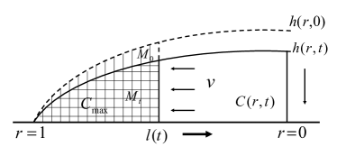
Figure 22: Sketch of the definition of $M_{0}$ and $M_{t}$.

We consider the change in total solute mass in the region $l(t)\leq r\leq 1$. Initially the amount of solute mass is

$$M_{0}=\int_{l(t)}^{1}2\pi C_{0}h(r,0)rdr.$$ (121)

For a position $r$ with $l(t)\leq r\leq 1$ when the moving front reaches $r$ at time $l^{-1}(r)$, the volume concentration at $r$ becomes $C_{\max}$ and the height at $r$ is $h(r,l^{-1}(r))$. The amount of solute mass near $r$ at time $l^{-1}(r)$ is thus $2\pi rC_{\max}h(r,l^{-1}(r))dr$. Since there is no horizontal movement of solute particles in the deposition region, this amount of mass does not change in time. Therefore at time $t$ the total amount of solute mass in the region $l(t)\leq r\leq 1$ is

$$M_{t}=\int_{l(t)}^{1}2\pi C_{\max}h(r,l^{-1}(r))rdr.$$ (122)

Conservation of solute mass demands that the change in total mass $M_{t}-M_{0}$ must be equal to the amount mass transported through $l(t)$ from time zero to time $t$, i.e.,

$$\int_{l(t)}^{1}2\pi C_{\max}h(r,l^{-1}(r))rdr-\int_{l(t)}^{1}2\pi C_{0}h(r,0)rdr=m(l(t),t),$$ (123)

$m(l(t),t)$ is defined by Eq. (34). We differentiate against $t$ on both sides of Eq. (123),

$$-2\pi lC_{\max}h(r,t)\frac{dl}{dt}+2\pi lC_{0}h(r,0)\frac{dl}{dt}=\frac{\partial m}{\partial t}+\frac{\partial m}{\partial l}\frac{dl}{dt},$$ (124)

and solve for $dl/dt$:

$$\frac{dl}{dt} =\frac{\partial m/\partial t}{2\pi l\left[C_{0}h(r,0)-C_{\max}h(r,t)\right]-\partial m/\partial l}$$

$$=-\left[\frac{l}{4(1-t)}\right]\frac{1}{\frac{C_{\max}\left(1-l^{2}\right)}{C_{0}\left[(1-t)^{-1/2}-l^{2}\right]}-1}.$$ (125)

Eq. (125) can also be written in the form:

$$\frac{dl}{dt}=-v\left(l,t\right)\frac{\delta}{1-\delta},$$ (126)

and we thus have re-covered Eq. (42).

The initial condition Eq. (43) can be proved via asymptotic expansion. Near the contact line $t$ is small, and we can write $l(t)=1-\alpha t+O(t^{2})$. Substituting this expression for $l(t)$ on both sides of Eq. (42) and retaining only the lowest order of $t$ in the limit $t\rightarrow 0$, we find

$$\alpha=\frac{1}{4}\frac{1}{\frac{4\alpha}{\delta_{0}(1+4\alpha)}-1},$$ (127)

We solve for $\alpha$:

$$\alpha=-\left.\frac{dl}{dt}\right|_{t=0}=\frac{1}{4}\frac{\sqrt{\delta_{0}}}{1-\sqrt{\delta_{0}}}.$$ (128)

The initial condition Eq. (43) is thus proved.

Eqs. (125) and (128) completely define the equation of the motion for the shock front.

References

- (1) T. F. Dupont, unpublished.
- (2) R. D. Deegan, O. Bakajin, T. F. Dupont, G. Huber, S. R. Nagel, and T. A. Witten, Nature 389, 827 (1997).
- (3) R. D. Deegan, Ph.D. Thesis (Dept. of Physics, University of Chicago, 1998).
- (4) R. D. Deegan, O. Bakajin, T. F. Dupont, G. Huber, S. R. Nagel, and T. A. Witten, Phys. Rev. E 62, 756 (2000).
- (5) R. D. Deegan, Phys. Rev. E 61, 475 (2000).
- (6) Y. O. Popov, Ph.D. Thesis (Dept. of Physics, University of Chicago, 2003).
- (7) Y. O. Popov, Phys. Rev. E 71, 036313 (2005).
- (8) J. Boneberg, F. Burmeister, C. Shafle, P. Leiderer, D. Reim, A. Fery, and S. Herminghaus, Langmuir 13, 7080 (1997).
- (9) T. Ondarcuhu and C. Joachim, Europhys. Lett. 42, 215 (1998).
- (10) E. Rabani, D. R. Reichman, P. L. Geissler, and L. E. Brus, Nature 426, 271 (2003).
- (11) A. Sommer, M. Ben-Moshe, and S. Magdassi, J. Phys. Chem. B 108, 8 (2004).
- (12) M. Abkarian, J. Nunes, and H. A. Stone, J. Am. Chem. Soc. 126, 5978 (2004).
- (13) Z. Lin and S. Granick, J. Am. Chem. Soc. 127, 2816 (2005).
- (14) S. Magdassi, M. Grouchko, D. Toker, A. Kamyshny, I. Balberg, and O. Millo, Langmuir 21, 10264 (2005).
- (15) R. G. Larson, T. T. Perkins, D. E. Smith, and S. Chu, Phys. Rev. E 55, 1794 (1997).
- (16) H. Hu and R. G. Larson, J. Phys. Chem. B, 106, 1334 (2002).
- (17) I. Smalyukh, O. Zribi, J. Butler, O. Lavrentovich, and G. Wong, Phys. Rev. Lett. 96, 177801 (2006).
- (18) N. V. Priezjev, A. A. Darhuber, and S. M. Troian, Phys. Rev. E 71, 041608 (2005).
- (19) T. Kajiya, E. Nishitani, T. Yamaue, and M. Doi, Phys. Rev. E 73, 011601 (2006).
- (20) K. D. Danov, N. Alleborn, H. Raszillier, and F. Durst, Phys. Fluids 10, 131 (1998).
- (21) Z. Mitov and E. Kumacheva, Phys. Rev. Lett. 81, 3427 (1998).
- (22) P. G. de Gennes, Eur. Phys. J. E 6, 421 (2001).
- (23) V. X. Nguyen and K. J. Stebe, Phys. Rev. Lett. 88, 164501 (2002).
- (24) E. Adachi, A. S. Dimitrov, and K. Nagayama, Langmuir 11, 1057 (1995).
- (25) L. Shmuylovich, A. Q. Shen, and H. A. Stone, Langmuir 18, 3441 (2002).
- (26) M. Nonomura, R. Kobayashi, Y. Nishiura, and M. Shimomura, J. Phys. Soc. Jpn. 72, 2468 (2003).
- (27) Y. O. Popov and T. A. Witten, Eur. Phys. J. E 6, 211 (2001).
- (28) Y. O. Popov and T. A. Witten, Phys. Rev. E 68, 036306 (2003).
- (29) R. Zheng, Y. O. Popov, and T. A. Witten, Phys. Rev. E 72, 046303 (2005).
- (30) T. F. Dupont, private communication.
- (31) B. J. Fisher, Langmuir 18, 60 (2002).
- (32) M. A. Ray, H. Kim, and L. Jia, Langmuir 21, 4786 (2005).
- (33) J. Xu, J. Xia, S. W. Hong, Z. Lin, F. Qiu, and Y. Yang, Phys. Rev. Lett. 96, 066104 (2006).
- (34) S. W. Hong, J. Xu, J. Xia, Z. Q. Lin, F. Qiu, and Y. L. Yang, Chem. Mater. 17, 6223 (2005).
- (35) T. A. Witten, Structured Fluids: Polymers, Colloids, Surfactants, Oxford University Press (2004).
- (36) P. G. de Gennes, Eur. Phys. J. E 7, 31 (2002).
- (37) R. Zheng and T. A. Witten, Phys. Rev. E 74, 051602 (2006).
- (38) P. G. de Gennes, Rev. Mod. Phys. 57, 827 (1985).
- (39) P. C. Ohara and W. M. Gelbart, Langmuir 14, 3418 (1998).
- (40) H. Nakanishi, Phys. Rev. E 73, 061603 (2006).
- (41) M. G. Nikolaides, A. R. Bausch, M. F. Hsu, A. D. Dinsmore, M. P. Brenner, C. Gay, and D. A. Weitz, Nature 420, 299 (2002).
- (42) E. A. van Nierop, M. A. Stijnman, and S. Hilgenfeldt, Europhys. Lett. 72, 671 (2005).
- (43) A. J. Liu and S. R. Nagel, Nature 396, 21 (1998).
- (44) E. Corwin, H. Jaeger, and S. R. Nagel, Nature 435, 1075 (2005).