A novel numerical technique used in the solution of ordinary differential equations with a mixture of integer and fractional derivatives

Abstract

Using both fractional derivatives, defined in the Riemann-Liouville and Caputo senses, and classical derivatives of the integer order we examine different numerical approaches to ordinary differential equations. Generally we formulate some algorithms where four discrete forms of the Caputo derivative and three different numerical techniques of solving ordinary differential equations are proposed. We then illustrate how to introduce classical initial conditions into equations where the Riemann-Liouville derivative is included.

1 Introduction

In the past, fractional calculus was applied only from a mathematical point of view. The fundamental work was done in [20, 21, 23, 25]. At present fractional calculus is extremely popular due to a rapid expansion in the field of practical applications. Such applications have been used in physics and mechanics [15, 28], finance [19, 26], hydrology [3, 27] and many other disciplines.

Ordinary differential equations including a mixture of integer and fractional derivatives are a natural extension of integer-order differential equations and give a novel approach to mathematical modeling many processes in nature. The solution of a equation strongly depends on form of the equation and is still considered by many authors. It should be noted that an analytical approach is limited to the linear form of equations and includes special functions such as Fox and Wright functions[12, 16] or the Mittag-Leffler function [25]. This greatly limits practical implementations, i.e. sometimes it is very difficult to illustrate the solution in one simple chart. On the other hand, a numerical solution [1, 7, 9, 10, 17] is an alternative approach to analytical one. However, this approach has many disadvantages, i.e. the introduction of the initial conditions included in the Riemann-Liouville derivative [14], the unreasonable assumption that a method applied to a single term equation is proper for solving a multi-term equation [8, 24] etc. Against this background Ford [9] noticed that there can be a considerable gap between methods that perform well in theory and those whose implementations are effective.

In this paper we try to propose a numerical approach which will be more convenient in practical applications. We will give a numerical procedure for how to introduce classical initial conditions into an equation where the Riemann-Liouville derivative is included. Here we will focus on such types of equation as

$$f\left({x,y\left(x\right),D^{1}y(x),\ldots,D^{p}y(x),D^{\alpha_{1}}y\left(x\right),\ldots,D^{\alpha_{m}}y\left(x\right)}\right)=0$$ (1)

where y(x) is the solution obtained for the class of continuous functions,
$D^{1}y(x),\ldots,D^{p}y(x)$ are derivatives of the integer order, $D^{\alpha_{1}}y(x),\ldots,D^{\alpha_{m}}y(x)$ are derivatives of the fractional order and $\alpha_{1},\ldots,\alpha_{m}\in R$ are real orders of a fractional derivative. We assume that the fractional derivative is defined as the left-side Caputo derivative [2]

$${}_{x_{0}}^{C}D_{x}^{\alpha}y\left(x\right)=\frac{1}{{\Gamma\left({n-\alpha}\right)}}\int\limits_{x_{0}}^{x}{\frac{{y^{\left(n\right)}\left(\tau\right)}}{{\left({x-\tau}\right)^{\alpha-n+1}}}d\tau}~{}~{}~{}~{}~{}~{}for~{}x>x_{0}$$ (2)

and the left-side Riemman-Liouville derivative [25]

$${}_{x_{0}}D_{x}^{\alpha}y\left(x\right)=\frac{1}{{\Gamma\left({n-\alpha}\right)}}\frac{{d^{n}}}{{dx^{n}}}\int\limits_{x_{0}}^{x}{\frac{{y\left(\tau\right)}}{{\left({x-\tau}\right)^{\alpha-n+1}}}d\tau}~{}~{}~{}~{}~{}~{}for~{}x>x_{0}$$ (3)

In above formulae, the notation $n=[\alpha]+1$ where $[\cdotp]$ is an integer part of a real number. Moreover, we introduce a definition of the left-side Riemann-Liouville fractional integral [21] as

$${}_{x_{0}}I_{x}^{\beta}y\left(x\right)=\frac{1}{{\Gamma\left(\beta\right)}}\int\limits_{x_{0}}^{x}{\frac{{y\left(\tau\right)}}{{\left({x-\tau}\right)^{1-\beta}}}}d\tau~{}~{}~{}~{}~{}~{}for~{}x>x_{0}$$ (4)

which will be used in our further calculations. Note that $\beta$ ($\beta>0$) is the real order of Eqn. (4). On the base of theory [21] we use an expression

$${}_{x_{0}}^{C}D_{x}^{\alpha}y\left(x\right)={}_{x_{0}}I_{x}^{n-\alpha}\left({D^{n}y\left(x\right)}\right)$$ (5)

which shows a relationship between the Caputo derivative (2) and the Riemann-Liouville integral (3). With regard to papers [1, 4, 9] in which numerical methods are used in the solution of fractional differential equations, the authors mostly use the Caputo derivative. However, there is a small number of papers [10] where the authors use the Riemann-Liouville derivative. This small number of papers were confronted by the problem of how to introduce classical initial conditions in the Riemann-Liouville derivative in order to obtain a solution for a class of continuous functions. In this paper, we propose a way to avoid this problem. To be more precise, in every equation where the Riemann-Liouville derivative occurs we will change it for the Caputo one. Following this we will discretize only the Caputo derivative, except for one case where the real number of the Riemann-Liouville derivative dominates in the equation. In this case we propose ${}_{x_{0}}D^{\alpha}_{x}y(x)=D^{n}{}_{x_{0}}I^{n-\alpha}_{x}y(x)$ and then discretize the left-side Riemann-Liouville integral ${}_{x_{0}}I^{n-\alpha}_{x}$.

2 Statement of the problem and its solution

With regard to Eqn. (1) we limit our considerations to the equation which has the following form

$$D^{p}y\left(x\right)+\lambda\left\{\begin{array}[]{l}{}_{x_{0}}^{C}D_{x}^{\alpha}y\left(x\right)\\ {}{}\\ {}_{x_{0}}D_{x}^{\alpha}y\left(x\right)\\ \end{array}\right.=0$$ (6)

where $p$ denotes an integer number being the derivatives order, $\alpha\in\langle 0,1)$ is the order of the fractional derivative and $\lambda$ is an arbitrary real number. This simple form of the equation allows us to show how our methods work properly in comparison to analytical solutions. Note that Eqn. (6) is the homogeneous ordinary differential equation with a mixture of derivatives. The function $y(x)$ being the solution of this equation, strongly belongs to the class of continuous functions. On the basis of our previous results [17] we rewrite Eqn. (6) in an explicit form. Consequently we obtain the three following types of equation:

• $p>n$ for $p=2$, $\alpha\in\ \langle 0,1)$, $n=1$

  $$D^{2}y\left(x\right)+\lambda{}_{x_{0}}^{C}D_{x}^{\alpha}y\left(x\right)=0$$ (7)

  $$D^{2}y\left(x\right)+\lambda{}_{x_{0}}D_{x}^{\alpha}y\left(x\right)=0$$ (8)

  It can be seen in above equations that the integer order of classical derivative dominates over the fractional one.

• $p=n$ for $p=1$, $\alpha\in\ \langle 0,1)$, $n=1$

  $$D^{1}y\left(x\right)+\lambda{}_{x_{0}}^{C}D_{x}^{\alpha}y\left(x\right)=0$$ (9)

  $$D^{1}y\left(x\right)+\lambda{}_{x_{0}}D_{x}^{\alpha}y\left(x\right)=0$$ (10)

  In this case we have equal integer orders for the classical and fractional derivative.

• $p<n$ for $p=0$, $\alpha\in\ \langle 0,1)$, $n=1$

  $${}_{x_{0}}^{C}D_{x}^{\alpha}y\left(x\right)+\lambda y\left(x\right)=0$$ (11)

  $${}_{x_{0}}D_{x}^{\alpha}y\left(x\right)+\lambda y\left(x\right)=0$$ (12)

  The last case shows fractional ordinary differential equations which are well known in the literature. It may observe that the fractional order of the equation dominates over the integer one.

2.1 Analytical solutions

To compare our direct numerical results we are obligated to solve the above system of equations in an analytical way. In this solution we will use a general idea which transforms the Riemann-Liouville derivative to the Caputo one [23]. Thus we have

$${}_{x_{0}}D_{x}^{\alpha}y\left(x\right)=\sum\limits_{i=0}^{n-1}{\frac{{\left({x-x_{0}}\right)^{i-\alpha}}}{{\Gamma\left({i-\alpha+1}\right)}}D^{i}y\left({x_{0}}\right)+{}_{x_{0}}^{C}D_{x}^{\alpha}y\left(x\right)}$$ (13)

On the base of [20] we also use the Laplace transform. Following that the transform of the derivative of the integer order $m\in N$ is

$$\mathcal{L}\left[{D^{m}y\left(x\right)}\right]=s^{m}F\left(s\right)-\sum\limits_{k=0}^{m-1}{s^{k}D^{m-k-1}y\left(x_{0}\right)}$$ (14)

The Laplace transform of the Caputo derivative is

$$\mathcal{L}\left[{{}_{x_{0}}^{C}D_{x}^{\alpha}y\left(x\right)}\right]=s^{\alpha}F\left(s\right)-\sum\limits_{k=0}^{n-1}{s^{\alpha-k-1}D^{k}y\left(x_{0}\right)}$$ (15)

Using (13) and (15) we calculated the Laplace transform from the Riemann-Liouville derivative in the following form

$$\begin{array}[]{c}\mathcal{L}\left[{{}_{x_{0}}D_{x}^{\alpha}y\left(x\right)}\right]=\mathcal{L}\left[{\sum\limits_{i=0}^{n-1}{\frac{{\left({x-x_{0}}\right)^{i-\alpha}}}{{\Gamma\left({i-\alpha+1}\right)}}D^{i}y\left({x_{0}}\right)+{}_{x_{0}}^{C}D_{x}^{\alpha}y\left(x\right)}}\right]=\\ {}{}\hfil\\ =\sum\limits_{i=0}^{n-1}{\frac{{D^{i}y\left({x_{0}}\right)}}{{\Gamma\left({i-\alpha+1}\right)}}\frac{{\Gamma\left({i-\alpha+1}\right)}}{{s^{i-\alpha+1}}}}+s^{\alpha}F\left(s\right)-\sum\limits_{j=0}^{n-1}{s^{\alpha-j-1}D^{j}y\left({x_{0}}\right)}=\\ {}{}\hfil\\ =s^{\alpha}F\left(s\right)\\ \end{array}$$ (16)

It should be noted that Eqn. (16) is limited by initial conditions which are omitted here. In previous considerations we assumed function $y(x)$ to be continuous. Therefore Eqn. (16) is contrary to the Laplace transform found in the literature [20] where initial conditions of non-integer order occur. This arises from an assumption that function $y(x)$ is non-continuous.

In our analytical solutions we use also two additional transforms as

$$\mathcal{L}\left[y\left(x\right)\right]=F\left(s\right)$$ (17)

$$\mathcal{L}\left[{x^{\alpha}}\right]=\frac{{\Gamma\left({\alpha+1}\right)}}{{s^{\alpha+1}}}$$ (18)

Using the above transforms in the set of equations (7)-(12) and retransforming the results we obtain analytical solutions. Including initial conditions

$$y\left(x_{0}\right)=y_{0},~{}~{}D^{1}y\left(x_{0}\right)=\mathop{y^{\prime}_{0}}$$ (19)

the analytical solution to Eqn. (7) is

$$\begin{array}[]{c}y\left(x\right)=y_{0}+\mathop{y^{\prime}_{0}}\left(x-x_{0}\right)E_{2-\alpha,2}\left({-\lambda\left(x-x_{0}\right)^{2-\alpha}}\right)\\ {}{}\hfil\\ D^{1}y\left(x\right)=\mathop{y^{\prime}_{0}}E_{2-\alpha,2}\left({-\lambda\left(x-x_{0}\right)^{2-\alpha}}\right)\\ +\mathop{y^{\prime}_{0}}\left({2-\alpha}\right)\left(x-x_{0}\right)E_{2-\alpha,2}^{\left(1\right)}\left({-\lambda\left(x-x_{0}\right)^{2-\alpha}}\right)\\ \end{array}$$ (20)

where $E_{\alpha,\beta}\left({-\lambda x^{\alpha}}\right)$ denotes the Mittag-Leffler function [25] which is defined as

$$E_{\alpha,\beta}\left({-\lambda x^{\alpha}}\right)=\sum\limits_{i=0}^{\infty}{\frac{{\left({-\lambda}\right)^{i}x^{\alpha i}}}{{\Gamma\left({\alpha i+\beta}\right)}}}$$ (21)

It should be noted that $E_{\alpha,\beta}^{\left(1\right)}\left({-\lambda x^{\alpha}}\right)$ occurs in solution (20), which is the first derivative of the Mittag-Leffler function (21) and is defined as

$$E_{\alpha,\beta}^{\left(1\right)}\left({-\lambda x^{\alpha}}\right)=\sum\limits_{i=1}^{\infty}{\frac{{\left({-\lambda}\right)^{i}ix^{\alpha i-1}}}{{\Gamma\left({\alpha i+\beta}\right)}}}$$ (22)

Solving Eqn. (8), where initial conditions (22) are included, we have

$$\begin{array}[]{c}y\left(x\right)=y_{0}E_{2-\alpha,1}\left({-\lambda\left(x-x_{0}\right)^{2-\alpha}}\right)\\ +\mathop{y^{\prime}_{0}}\left(x-x_{0}\right)E_{2-\alpha,2}\left({-\lambda\left(x-x_{0}\right)^{2-\alpha}}\right)\\ {}{}\hfil\\ D^{1}y\left(x\right)=\left({2-\alpha}\right)y_{0}E_{2-\alpha,1}^{\left(1\right)}\left({-\lambda\left(x-x_{0}\right)^{2-\alpha}}\right)\\ ~{}+\mathop{y^{\prime}_{0}}E_{2-\alpha,2}\left({-\lambda\left(x-x_{0}\right)^{2-\alpha}}\right)\\ +\left({2-\alpha}\right)\mathop{y^{\prime}_{0}}\left(x-x_{0}\right)E_{2-\alpha,2}^{\left(1\right)}\left({-\lambda\left(x-x_{0}\right)^{2-\alpha}}\right)\\ \end{array}$$ (23)

Eqn. (9) with the initial condition $y(x_{0})=y_{0}$ has the following solution

$$y\left(x\right)=y_{0}$$ (24)

Eqn. (10) with the initial condition $y(x_{0})=y_{0}$ has the following solution

$$y\left(x\right)=y_{0}E_{1-\alpha,1}\left({-\lambda\left(x-x_{0}\right)^{1-\alpha}}\right)$$ (25)

Eqn. (11) with the initial condition $y(x_{0})=y_{0}$ has the following solution

$$y\left(x\right)=y_{0}E_{\alpha,1}\left({-\lambda\left(x-x_{0}\right)^{\alpha}}\right)$$ (26)

However Eqn. (12) with the initial condition $y(x_{0})=y_{0}$ has a trivial solution in the following form

$$y\left(x\right)=0$$ (27)

The above solution, arises from our assumption that we only consider a class of continuous functions $y(x)$. In our next considerations we neglect this solution. It can be seen in literature [9, 10] that the authors solve a similar type of equation to Eqn. (12), where an exciting function $f(x)$ is added on the right side of the equation.

2.2 Discrete forms of the Caputo derivative

There are many propositions on papers [7, 13, 21], how to discretize fractional operators. Basically several discrete forms are employed to take into account the different form of the function included in the fractional derivative. In this subsection we would like to propose a general procedure for how to discretize the function. Let us consider an independent value $x$ which occurs on a length of calculations $\langle x_{0},x_{N}\rangle$, where $x_{0}$ and $x_{N}$ are the beginning and end of the range respectively. We introduce a homogeneous grid $x_{0}<x_{1}<\ldots<x_{N}$. Fig. 1 shows four discrete forms of a derivative $D^{n}y(x)=B$ which is included in the Caputo derivative (2).

Taking into account the above discrete forms of the integer derivative we propose the following discrete schemes of the Caputo derivative (2) as:

• the left-side form (case-I)

  $$\begin{array}[]{c}{}_{x_{0}}^{C}D_{x}^{\alpha}y\left(x\right)\cong\\ \cong\frac{1}{{\Gamma\left({n-\alpha+1}\right)}}\sum\limits_{k=1}^{N}{B_{k-1}\left[{\left({x_{N}-x_{k-1}}\right)^{n-\alpha}-\left({x_{N}-x_{k}}\right)^{n-\alpha}}\right]}\end{array}$$ (28)

  where $x\in\langle x_{k-1},x_{k}\rangle$ and $D^{n}y\left(x_{k-1}\right)=B_{k-1}$,

• the right-side form (case-II)

  $$\begin{array}[]{c}{}_{x_{0}}^{C}D_{x}^{\alpha}y\left(x\right)\cong\\ \cong\frac{1}{{\Gamma\left({n-\alpha+1}\right)}}\sum\limits_{k=1}^{N}{B_{k}\left[{\left({x_{N}-x_{k-1}}\right)^{n-\alpha}-\left({x_{N}-x_{k}}\right)^{n-\alpha}}\right]}\end{array}$$ (29)

  where $x\in\langle x_{k-1},x_{k}\rangle$ and $D^{n}y\left(x_{k}\right)=B_{k}$,

• the middle-side form (case-III)

  $$\begin{array}[]{c}{}_{x_{0}}^{C}D_{x}^{\alpha}y\left(x\right)\cong\\ \cong\frac{1}{{\Gamma\left({n-\alpha+1}\right)}}\sum\limits_{k=1}^{N}{\frac{B_{k}+B_{k-1}}{2}\left[{\left({x_{N}-x_{k-1}}\right)^{n-\alpha}-\left({x_{N}-x_{k}}\right)^{n-\alpha}}\right]}\end{array}$$ (30)

  where $x\in\langle x_{k-1},x_{k}\rangle$ and $\frac{D^{n}y\left(x_{k}\right)+D^{n}y\left(x_{k-1}\right)}{2}=\frac{B_{k}+B_{k-1}}{2}$.

• the linear form taken from [18] (case-IV)

  $$\begin{array}[]{c}{}_{x_{0}}^{C}D_{x}^{\alpha}y\left(x\right)\cong\\ \cong\frac{1}{{\Gamma\left({n-\alpha}\right)}}\sum\limits_{k=1}^{N}{\left\{{\frac{{A_{k}}}{{n+1-\alpha}}\left[{\left({x_{N}-x_{k}}\right)^{n+1-\alpha}\left({x_{N}-x_{k-1}}\right)^{n+1-\alpha}}\right]}\right.}\\ +\left.{\frac{{A_{k}x_{N}+B_{k}}}{{n-\alpha}}\left[{\left({x_{N}-x_{k-1}}\right)^{n-\alpha}-\left({x_{N}-x_{k}}\right)^{n-\alpha}}\right]}\right\}\\ \end{array}$$ (31)

  where $A_{k}=\frac{D^{n}y\left(x_{k}\right)-D^{n}y\left(x_{k-1}\right)}{x_{k}-x_{k-1}}$, $B_{k}=D^{n}y\left(x_{k}\right)-A_{k}x_{k}$.

We try to use the above forms in numerical schemes to solve ordinary differential equations. It should be noted that Eqn. (28) (case I) is useful in the explicit scheme as, for example, the Euler’s method [22]. The next discrete forms predicted by formulae (29) (30) and (31) can use for any predictor-corrector method [22].

Additionally, we also propose a discrete form of the Riemann-Liouville fractional integral (4). We consider a range $\langle x_{k-1},x_{k}\rangle~{}\left(k=1,\ldots,N\right)$ for $k=1,\ldots,N$ and we assume a constant value of function $y(x_{k})=B_{k}$. In this case the integral operator (4) has the following form

$${}_{x_{0}}I_{x}^{\beta}y\left(x\right)\cong\frac{1}{{\Gamma\left({\beta+1}\right)}}\left[{B_{1}\left({x_{N}-x_{0}}\right)+\sum\limits_{k=2}^{N}{\left({B_{k}-B_{k-1}}\right)\left({x_{N}-x_{k-1}}\right)^{\beta}}}\right]$$ (32)

where $B_{k}=y\left(x_{k}\right)$.

2.3 Numerical methods of solving ordinary differential equations

In this paper, we chose only three numerical methods which are used in the literature to solve an initial-value problem for ordinary differential equations.

The Euler’s method [22] is an explicit one-step method. Using this method for any ordinary differential equation of the first order we obtain

$$y_{k}=y_{k-1}+hf\left({x_{k-1},y_{k-1}}\right),~{}~{}k=1,\ldots,N$$ (33)

The Adams method [22] of the fourth order is the most popular method in the literature [5, 6] which is used to solve fractional differential equations. This is a predictor-corrector method. It should be noted that for the method of fourth order we have to determine three beginning values $y_{1},y_{2},y_{3}$ of the function. This can be done by using, for example, the Euler’s method. The Adams method for a differential equation of the first order has the following form:

• the predictor stage

  $${}^{pr}y_{k}=y_{k-1}+h\left({\frac{{55}}{{24}}f_{k-1}-\frac{{59}}{{24}}f_{k-2}+\frac{{37}}{{24}}f_{k-3}-\frac{9}{{24}}f_{k-4}}\right)$$ (34)

• the corrector stage

  $${}^{cr}y_{k}=y_{k-1}+h\left({\frac{{19}}{{24}}f_{k-1}-\frac{5}{{24}}f_{k-2}+\frac{1}{{24}}f_{k-3}}\right)+\frac{9}{{24}}hf_{k}$$ (35)

  where $f_{k}=f\left({x_{k},{}^{pr}y_{k}}\right),~{}~{}f_{k-j}=f\left({x_{k-j},y_{k-j}}\right),~{}~{}j=1,\ldots,4,\\ k=4,\ldots,N$

The Gear’s method [11] is also a predictor-corrector type method. This method has an advantage in cases where only one call of the function is required in one step of the calculation. However, it needs higher derivatives in the algebraic form at the beginning point $x_{0}$. This is a disadvantage of the method. The Gear’s method for ordinary differential equations of the first order is defined as

• in the predictor stage

  $${}^{pr}D^{i}y_{k}=\sum\limits_{j=0}^{5}{P_{j-i}D^{j}y_{k-1}}$$ (36)

  where $P_{l}=\left\{\begin{array}[]{l}0~{}~{}\mbox{for}~{}~{}l=-5,\ldots,-1\\ \frac{{h^{l}}}{{l!}}~{}~{}\mbox{for}~{}~{}l=0,\ldots,5\\ \end{array}\right.$ and $i=0,\ldots,5$, $k=1,\ldots,N$

• in the corrector stage

  $${}^{cr}D^{i}y_{k}={}^{pr}D^{i}y_{k}+\frac{{i!}}{{2h^{i-2}}}c_{i}\Delta{}^{cr}D^{2}y_{k}$$ (37)

  where $\Delta{}^{cr}D^{2}y_{k}={}^{cr}D^{2}y_{k}-{}^{pr}D^{2}y_{k}$, ${}^{cr}D^{2}y_{k}=f\left(x_{k},y_{k},{}^{pr}D^{1}y_{k}\right)$
  for $k=1,\ldots,N$, $i=0,\ldots,5$
    
  and coefficients are defined as
  $c_{0}=\frac{3}{16},c_{1}=\frac{251}{360},c_{2}=1,c_{3}=\frac{11}{18},c_{4}=\frac{1}{6},c_{5}=\frac{1}{60}$.
    
  

All the considered methods will be used in the next sections in order to construct algorithms.

2.4 Algorithms

In this subsection, we propose several algorithms which solve a set of ordinary differential equations presented by general formula (6).

Algorithm 1.1

At the beginning we consider Eqn. (7) with initial conditions (19). On the base of the Euler’s method (33) and the left-side discrete form (28) (case-I) of Caputo derivative we then propose the following algorithm

• Prediction of necessary data: initial conditions, the fractional order $\alpha\in\langle 0,1)$, the total length of calculations $x\in\langle x_{0},x_{N}\rangle$, the step of calculations $h$.

• Governing calculations: let $k=1,\ldots,N$ then

  $$\begin{array}[]{l}{}_{x_{0}}^{C}D_{x}^{\alpha}y_{k}=\frac{1}{{\Gamma\left({2-\alpha}\right)}}\sum\limits_{j=1}^{k}{D^{1}y_{k-1}\left[{\left({x_{k}-x_{j-1}}\right)^{1-\alpha}-\left({x_{k}-x_{j}}\right)^{1-\alpha}}\right]}\\ {}{}\\ y_{k}=y_{k-1}+hD^{1}y_{k-1}\\ {}{}\\ D^{1}y_{k}=D^{1}y_{k-1}-h\lambda{}_{x_{0}}^{C}D_{x}^{\alpha}y_{k}\\ \end{array}$$ (38)

Algorithm 1.2

Considering the same differential equation as presented in Algorithm 1.1 we present another approach. This is based on the Adams method (34) (35) and includes the linear-discrete form (31) (case-IV) of the Caputo derivative. Thus we have

• prediction of necessary data: initial conditions, the fractional order $\alpha\in\langle 0,1)$, the total length of calculations $x\in\langle x_{0},x_{N}\rangle$, the step of calculations h and additionally ${}^{C}_{x_{0}}D^{\alpha}_{x}y_{0}=0$.

• Introductory calculations: three initial values of the function $y_{1},y_{2},y_{3}$ are calculated by the Euler’s method (algorithm 1.1).

• Governing calculations: let $k=4,\ldots,N$ then the predictor stage is

  $$\begin{array}[]{c}{}^{pr}y_{k}=y_{k-1}+h\left({\frac{{55}}{{24}}D^{1}y_{k-1}-\frac{{59}}{{24}}D^{1}y_{k-2}+\frac{{37}}{{24}}D^{1}y_{k-3}-\frac{9}{{24}}D^{1}y_{k-4}}\right)\\ {}{}\hfil\\ {}^{pr}D^{1}y_{k}=D^{1}y_{k-1}\\ -h\lambda\left({\frac{{55}}{{24}}{}_{x_{0}}^{C}D_{x}^{\alpha}y_{k-1}-\frac{{59}}{{24}}{}_{x_{0}}^{C}D_{x}^{\alpha}y_{k-2}+\frac{{37}}{{24}}{}_{x_{0}}^{C}D_{x}^{\alpha}y_{k-3}-\frac{9}{{24}}{}_{x_{0}}^{C}D_{x}^{\alpha}y_{k-4}}\right)\\ \end{array}$$ (39)

  
  
  

  $$\begin{array}[]{c}{}_{x_{0}}^{C}D_{x}^{\alpha}y_{k}=\\ =\frac{1}{{\Gamma\left({1-\alpha}\right)}}\sum\limits_{j=1}^{k}\bigg{\{}\frac{{D^{1}y_{j}-D^{1}y_{j-1}}}{{\left({2-\alpha}\right)h}}\left[{\left({x_{k}-x_{j}}\right)^{2-\alpha}-\left({x_{k}-x_{j-1}}\right)^{2-\alpha}}\right]\\ +\frac{{\left({D^{1}y_{j}-D^{1}y_{j-1}}\right)\left({x_{k}-x_{j}}\right)+hD^{1}y_{j}}}{{\left({1-\alpha}\right)h}}\left[{\left({x_{k}-x_{j-1}}\right)^{1-\alpha}-\left({x_{k}-x_{j}}\right)^{1-\alpha}}\right]\bigg{\}}\\ \end{array}$$ (40)

  
  
  

  and the corrector stage is

  $$\begin{array}[]{c}{}^{cr}y_{k}=y_{k-1}+h\left({\frac{{19}}{{24}}D^{1}y_{k-1}-\frac{5}{{24}}D^{1}y_{k-2}+\frac{1}{{24}}D^{1}y_{k-3}}\right)\\ +\frac{9}{{24}}hD^{1}y_{k}\\ {}{}\hfil\\ {}^{cr}D^{1}y_{k}=D^{1}y_{k-1}\\ -h\lambda\left({\frac{{19}}{{24}}{}_{x_{0}}^{C}D_{x}^{\alpha}y_{k-1}-\frac{5}{{24}}{}_{x_{0}}^{C}D_{x}^{\alpha}y_{k-2}+\frac{1}{{24}}{}_{x_{0}}^{C}D_{x}^{\alpha}y_{k-3}}\right)-\frac{9}{{24}}h\lambda{}_{x_{0}}^{C}D_{x}^{\alpha}y_{k}\\ \end{array}$$ (41)

It should be noted that additional assumptions, as shown by step 2 and step 3, need to be made for correct calculations to be achieved.

Algorithm 1.3

Still considering Eqn. (7) with initial conditions (19) we can present another approach in comparison to previous ones. This uses the Gear’s method (36) (37) and the middle-side discrete form (30) (case-III) of Caputo derivative.

• Prediction of necessary data: initial conditions, the fractional order $\alpha\in\langle 0,1)$, the total length of calculations $x\in\langle x_{0},x_{N}\rangle$, the step of calculations $h$ and additionally $D^{2}y_{0}=D^{3}y_{0}=D^{4}y_{0}=$ $=D^{5}y_{0}=0$.

• Governing calculations: let $k=1,\ldots,N$ then Eqn. (36) is the predictor stage and beginning of the correction stage is

  $$\begin{array}[]{l}{}_{x_{0}}^{C}D_{x}^{\alpha}y_{k}=\frac{1}{{\Gamma\left({2-\alpha}\right)}}\sum\limits_{j=1}^{k}{\frac{{D^{1}y_{k}+D^{1}y_{k-1}}}{2}\left[{\left({x_{k}-x_{j-1}}\right)^{1-\alpha}-\left({x_{k}-x_{j}}\right)^{1-\alpha}}\right]}\\ {}{}\\ \Delta{}^{cr}D^{2}y_{k}=-\lambda{}_{x_{0}}^{C}D_{x}^{\alpha}y_{k}-{}^{pr}D^{2}y_{k}\end{array}$$ (42)

  and it follows that we apply the correction stage given by Eqn. (37).

Algorithm 2.1

Now let us consider Eqn. (8) with initial conditions (19). It should be noted that this type of equation includes the Riemann-Liouville derivative. We apply the Euler’s method (33) and Eqn. (13) which transforms the Riemann-Liouville derivative to the Caputo one. It should be remembered that Eqn. (13) includes a set of initial conditions in the general form $\sum\limits_{i=0}^{n-1}{\frac{{\left({x-x_{0}}\right)^{i-\alpha}}}{{\Gamma\left({i-\alpha+1}\right)}}}D^{i}y\left({x_{0}}\right)$. In the case of the lower limit $x$ tends to $x_{0}$ and then the above expression is infinite. This means that we cannot use a full numerical approach in order to solve the class of ordinary differential equations where the Riemann-Liouville derivative is included. However an assumption of homogeneous initial conditions i.e. $D^{I}y\left(x_{0}\right)=0$ avoids the problem. Eqn. (8) has a correct analytical solution (23) and the function $y(x)$ has a finite value at the beginning point $x_{0}$ which is contrary to previous considerations. With regard to our assumption that function $y(x)$ belongs to the class of continuous functions we are obligated to improve the factor $\left(x-x_{0}\right)^{i-\alpha}$ included in Eqn. (13) in order to restrict the function continuity. Therefore we put $\left(x^{*}-x_{0}\right)^{i-\alpha}$ into Eqn. (13) instead of $\left(x-x_{0}\right)^{i-\alpha}$ where $x^{*}=x+c$ and $c=\left(\Gamma\left(1-\alpha\right)\right)^{-\alpha^{-1}}$. Point $c$ is where the shift from initial conditions to homogeneous initial conditions occurs. Our assumption allows for the correct behaviour of factor $\left(x^{*}-x_{0}\right)^{i-\alpha}=\left(x+c-x_{0}\right)^{i-\alpha}$ in Eqn. (13) in the class of continuous functions especially when $x$ tends to $x_{0}$. Taking into account the above considerations we have the following algorithm

• prediction of necessary data: initial conditions, the fractional order $\alpha\in\langle 0,1)$, the total length of calculations $x\in\langle x_{0},x_{N}\rangle$, the step of calculations $h$.

• Governing calculations: let $k=1,\ldots,N$ then

  $$\begin{array}[]{c}{}_{x_{0}}D_{x}^{\alpha}y_{k}=\frac{{\left({x_{k-1}^{*}-x_{0}}\right)^{-\alpha}}}{{\Gamma\left({1-\alpha}\right)}}y_{0}\\ +\frac{1}{{\Gamma\left({2-\alpha}\right)}}\sum\limits_{j=1}^{k}{D^{1}y_{k-1}\left[{\left({x_{k}-x_{j-1}}\right)^{1-\alpha}-\left({x_{k}-x_{j}}\right)^{1-\alpha}}\right]}\\ {}{}\hfil\\ y_{k}=y_{k-1}+hD^{1}y_{k-1}\\ {}{}\hfil\\ D^{1}y_{k}=D^{1}y_{k-1}-h\lambda{}_{x_{0}}D_{x}^{\alpha}y_{k}\\ \end{array}$$ (43)

  where $x_{k-1}^{*}=x_{k-1}+hc$.

Algorithm 2.2

The Euler’s method has been used in algorithm 2.1. Considering Eqn. (8) with initial conditions (19) and using the Adams method (34) with the linear-discrete form (31) (case-IV) of Caputo derivative we obtain

• prediction of necessary data: initial conditions, the fractional order $\alpha\in\langle 0,1)$, the total length of calculations $x\in\langle x_{0},x_{N}\rangle$, the step of calculations $h$, ${}^{C}_{x_{0}}D^{\alpha}_{x}y_{0}=0$ and $c=\left(\Gamma\left(1-\alpha\right)\right)^{-\alpha^{-1}}$.

• Introductory calculations: three initial values of the function $y_{1},y_{2},y_{3}$ are calculated by the Euler’s method (algorithm 2.1).

• Governing calculations: let $k=4,\ldots,N$ then the predictor stage is

  $$\begin{array}[]{c}{}^{pr}y_{k}=y_{k-1}+h\left({\frac{{55}}{{24}}D^{1}y_{k-1}-\frac{{59}}{{24}}D^{1}y_{k-2}+\frac{{37}}{{24}}D^{1}y_{k-3}-\frac{9}{{24}}D^{1}y_{k-4}}\right)\\ {}{}\hfil\\ {}^{pr}D^{1}y_{k}=D^{1}y_{k-1}\\ -h\lambda\left({\frac{{55}}{{24}}{}_{x_{0}}D_{x}^{\alpha}y_{k-1}-\frac{{59}}{{24}}{}_{x_{0}}D_{x}^{\alpha}y_{k-2}+\frac{{37}}{{24}}{}_{x_{0}}D_{x}^{\alpha}y_{k-3}-\frac{9}{{24}}{}_{x_{0}}D_{x}^{\alpha}y_{k-4}}\right)\\ \end{array}$$ (44)

  $$\begin{array}[]{c}{}_{x_{0}}D_{x}^{\alpha}y_{k}=\frac{{\left({x_{k-1}^{*}-x_{0}}\right)^{-\alpha}}}{{\Gamma\left({1-\alpha}\right)}}y_{0}\\ +\frac{1}{{\Gamma\left({1-\alpha}\right)}}\sum\limits_{j=1}^{k}\bigg{\{}\frac{{D^{1}y_{j}-D^{1}y_{j-1}}}{{\left({2-\alpha}\right)h}}\left[{\left({x_{k}-x_{j}}\right)^{2-\alpha}-\left({x_{k}-x_{j-1}}\right)^{2-\alpha}}\right]\\ +\frac{{\left({D^{1}y_{j}-D^{1}y_{j-1}}\right)\left({x_{k}-x_{j}}\right)+hD^{1}y_{j}}}{{\left({1-\alpha}\right)h}}\left[{\left({x_{k}-x_{j-1}}\right)^{1-\alpha}-\left({x_{k}-x_{j}}\right)^{1-\alpha}}\right]\bigg{\}}\\ \end{array}$$ (45)

  and the corrector stage is

  $$\begin{array}[]{c}{}^{cr}y_{k}=y_{k-1}+h\left({\frac{{19}}{{24}}D^{1}y_{k-1}-\frac{5}{{24}}D^{1}y_{k-2}+\frac{1}{{24}}D^{1}y_{k-3}}\right)+\frac{9}{{24}}hD^{1}y_{k}\\ {}{}\hfil\\ {}^{cr}D^{1}y_{k}=D^{1}y_{k-1}+\\ -h\lambda\left({\frac{{19}}{{24}}{}_{x_{0}}D_{x}^{\alpha}y_{k-1}-\frac{5}{{24}}{}_{x_{0}}D_{x}^{\alpha}y_{k-2}+\frac{1}{{24}}{}_{x_{0}}D_{x}^{\alpha}y_{k-3}}\right)-\frac{9}{{24}}h\lambda{}_{x_{0}}D_{x}^{\alpha}y_{k}\\ \end{array}$$ (46)

Algorithm 2.3

We present another algorithm on the base of Algorithms 2.1 and 2.2. We still consider Eqn. (8) with the initial conditions (19) and then we use the Gear’s method (36) (37) with the middle-side discrete form (30) (case-III) of Caputo derivative. We have

• prediction of necessary data: initial conditions, the fractional order $\alpha\in\langle 0,1)$, the total length of calculations $x\in\langle x_{0},x_{N}\rangle$, the step of calculations $h$, $c=\left(\Gamma\left(1-\alpha\right)\right)^{-\alpha^{-1}}$ and $D^{2}y_{0}=D^{3}y_{0}=$ $=D^{4}y_{0}=D^{5}y_{0}=0$.

• Governing calculations: let $k=1,\ldots,N$ then Eqn. (36) is the predictor stage and beginning of the correction stage is

  $$\begin{array}[]{c}{}_{x_{0}}D_{x}^{\alpha}y_{k}=\frac{1}{{\Gamma\left({2-\alpha}\right)}}\sum\limits_{j=1}^{k}{\frac{{D^{1}y_{k}+D^{1}y_{k-1}}}{2}\left[{\left({x_{k}-x_{j-1}}\right)^{1-\alpha}-\left({x_{k}-x_{j}}\right)^{1-\alpha}}\right]}\\ {}{}\hfil\\ \Delta{}^{cr}D^{2}y_{k}=-\lambda{}_{x_{0}}D_{x}^{\alpha}y_{k}-{}^{pr}D^{2}y_{k}\end{array}$$ (47)

  
  

  and it follows that we apply the correction stage given by Eqn. (37).

Algorithm 3.1

Next we consider another class of ordinary differential equations given by formula (9) with the initial condition $y(x_{0})=y_{0}$. Using the Euler’s method (33) and the left-side discrete form (28) (case-I) of the Caputo derivative we then propose the following algorithm

• prediction of necessary data: initial conditions, the fractional order $\alpha\in\langle 0,1)$, the total length of calculations $x\in\langle x_{0},x_{N}\rangle$, the step of calculations $h$ and $D^{1}y_{0}=0$.

• Governing calculations: let $k=1,\ldots,N$ then

  $$\begin{array}[]{c}{}_{x_{0}}^{C}D_{x}^{\alpha}y_{k}=\frac{1}{{\Gamma\left({2-\alpha}\right)}}\sum\limits_{j=1}^{k}{D^{1}y_{k-1}\left[{\left({x_{k}-x_{j-1}}\right)^{1-\alpha}-\left({x_{k}-x_{j}}\right)^{1-\alpha}}\right]}\\ {}{}\hfil\\ y_{k}=y_{k-1}-h\lambda{}_{x_{0}}^{C}D_{x}^{\alpha}y_{k-1}\\ {}{}\hfil\\ D^{1}y_{k}=-\lambda{}_{x_{0}}^{C}D_{x}^{\alpha}y_{k}\\ \end{array}$$ (48)

To simplify our considerations we neglect other algorithms which can be applied to solve Eqn. (9). On the basis of previous explanations of predictor-corrector methods one can construct interesting procedures self-reliantly.

Algorithm 4.1

Using the Euler’s method (33) and the left-side discrete form (28) (case-I) of the Caputo derivative we construct an algorithm which solves Eqn. (10) with the initial condition $y\left(x_{0}\right)=y_{0}$. Thus we obtain

• prediction of necessary data: initial conditions, the fractional order $\alpha\in\langle 0,1)$, the total length of calculations $x\in\langle x_{0},x_{N}\rangle$, the step of calculations $h$, $D^{1}y_{0}=0$ and $c=\left(\Gamma\left(1-\alpha\right)\right)^{-\alpha^{-1}}$.

• Governing calculations: let $k=1,\ldots,N$ then

  $$\begin{array}[]{c}{}_{x_{0}}D_{x}^{\alpha}y_{k}=\frac{{\left({x_{k-1}^{*}-x_{0}}\right)^{-\alpha}}}{{\Gamma\left({1-\alpha}\right)}}y_{0}\\ +\frac{1}{{\Gamma\left({2-\alpha}\right)}}\sum\limits_{j=1}^{k}{D^{1}y_{k-1}\left[{\left({x_{k}-x_{j-1}}\right)^{1-\alpha}-\left({x_{k}-x_{j}}\right)^{1-\alpha}}\right]}\\ {}{}\hfil\\ y_{k}=y_{k-1}-h\lambda{}_{x_{0}}D_{x}^{\alpha}y_{k-1}\\ {}{}\hfil\\ D^{1}y_{k}=-\lambda{}_{x_{0}}D_{x}^{\alpha}y_{k}\\ \end{array}$$ (49)

  where $x_{k-1}^{*}=x_{k-1}+hc$.

We also neglect other constructions of algorithms.

Algorithm 5.1

Using the Euler’s method (33) we solve numerically the last equation (11) taking into account the initial condition $y\left(x_{0}\right)=y_{0}$. Follow the discrete form of the Riemann-Liouville fractional integral (32) we have

• prediction of necessary data: initial conditions, the fractional order $\alpha\in\langle 0,1)$, the total length of calculations $x\in\langle x_{0},x_{N}\rangle$, the step of calculations $h$.

• Governing calculations: let $k=1,\ldots,N$ then

  $$\begin{array}[]{c}B_{k}=h^{\alpha-1}\bigg{\{}-\lambda\Gamma\left({2-\alpha}\right)y_{k-1}\\ -\sum\limits_{j=2}^{k}{B_{j-1}\left[{\left({x_{k}-x_{j-2}}\right)^{1-\alpha}\left({x_{k}-x_{j-1}}\right)^{1-\alpha}}\right]}\bigg{\}}\\ {}{}\hfil\\ y_{k}=y_{k-1}+hB_{k}\end{array}$$ (50)

In summary we propose numerical schemes suitable for all possible cases of Eqn. (6). We then generally apply two approaches. One is connected with the explicit method and the second is based on the predictor-corrector scheme. It should be noted that we illustrate all the considered methods (the Euler’s method, the Adams method and the Gear’s method) which are used in Eqns (7) (8). However we limit this illustration in Eqn. (9)-(11) only to the Euler’s method. In this case we omit the predictor-corrector methods because there are problems with applications. Using this approach we found that the Adams method requires known values of the first derivative in the algebraic form. However the Gear’s method requires the algebraic form of the second derivative which is used in calculations of the correction factor.

3 Results

The algorithms presented in the previous section allow us to compare numerical and analytical results respectively. First we compare the results obtained from four discrete forms of the Caputo derivative. Thus we assume a function

$$y\left(x\right)=x^{2}$$ (51)

where the Caputo derivative is

$$g(x)={}_{x_{0}}^{C}D_{x}^{\alpha}x^{2}=\frac{{\Gamma\left(3\right)x^{2-\alpha}}}{{\Gamma\left({3-\alpha}\right)}}$$ (52)

Table 1 shows analytical values of the function (52) at assumed points. The other rows of this table present the difference between the numerical and analytical results. Analysing this table we can see that the liner-discrete form of the Caputo derivative (31) (case-IV) gives the best results. However, this discrete form is very complex. This is a disadvantage of case-IV. It should be noted that the middle-side form (30) (case-III) also gives quite small errors. The next two discrete forms (28) and (29) generate large errors in comparison to the previous cases.

We try to estimate how several discrete forms of the Caputo derivative work in numerical schemes used to solve ordinary differential equations. It should be remembered that, as presented in subsection 2.4, there are many constructions of numerical approaches which are dependent on the form of the ordinary differential equation, the discrete form of the Caputo derivative assumed (cases I to IV) and, finally, on the numerical scheme (the explicit or predictor-correct schemes) used. Therefore, a general question arises: how to efficiently compare all the possible constructions of numerical schemes in order to comment on their practical application? First of all, we started our comparison between predictor-corrector methods. We can apply three forms of the Caputo derivative (cases II to IV) and two numerical schemes (the Adams and Gear’s schemes) as presented in the previous section. Let us start with Eqn. (7) where initial conditions

$$y\left(0\right)=0,~{}~{}D^{1}y\left(0\right)=1$$ (53)

are assumed. Note that Eqn. (7) has an analytical solution (20).

Table 2 presents a direct comparison of the two predictor-corrector methods where three discrete forms of the Caputo derivative for each method are included. It should be noted that we obtained many sets of data. Brief analysis presents the best results in the linear-discrete form (case-IV) (31) of the Caputo derivative for both the Gear’s (36) (37) and Adams (34) (35) methods. Satisfactory results can be also achieved by the application of the middle-side form (case-III) (30) obviously used for both methods. Taking into account the complexity of the forms, we chose the middle-side form (30) for the next calculations using the predictor-corrector method. We also noticed that the Gear’s method (36) (37) generates smaller error values than the Adams method (34) (35).

$$y\left(0\right)=-1,~{}~{}D^{1}y\left(0\right)=1$$ (54)

Now we consider all the numerical methods used to solve the same equation (7) with initial conditions (54). Fig. 2 illustrates the analytical solution taking into account the influence of parameter $\alpha$. Notice that for such a solution we used algorithms 1.1, 1.2 and 1.3 respectively. Table 3 presents the analytical values given by formula (20) and errors given by several algorithms used. It can be observed that the Gear’s method (algorithm 1.3) generates the smallest errors in comparison to other methods used. However, the Euler’s method (algorithm 1.1) performs better than the Adams method (algorithm 1.2). As we noted in the previous section, predictor-corrector methods have some disadvantages which are revealed in the calculations of higher derivatives for the Gear’s method or necessary values of the function at the initial three points for the Adams method. Moreover, a discrete form of the Caputo derivative has less of an influence on error calculations than a numerical method used in solving an ordinary differential equation.

Next we consider all the numerical methods used to solve of Eqn. (8) with initial conditions

$$y\left(0\right)=1,~{}~{}D^{1}y\left(0\right)=1$$ (55)

This equation has an analytical solution given by formula (23) It should be noted that for a such solution we used algorithms 2.1, 2.2 and 2.3 respectively. Fig. 3 shows the behavior of the analytical solution over an independent value $x$ for different values of the parameter $\alpha$. Table 4 presents analytical values given by formula (23) and errors given by several algorithms used. This numerical solution confirms our previous considerations that the Euler’s and Gear’s methods show the smallest errors. Taking into account both the errors generated by the numerical method and the complexity of numerical schemes we chose the Euler’s method as the method to use in the next calculations.

Assuming the initial condition $y\left(0\right)=2$ for Eqn. (9) we obtain an analytical solution in the form

$$y\left(x\right)=2$$ (56)

Fig. 4 shows direct comparison between analytical solution (56) and the Euler’s method (algorithm 3.1) for Eqn. (9). In this case we have not printed a table because only a very small difference between the analytical and numerical solutions can be observed.

Next we consider Eqn. (10) with the initial condition $y(0)=1$. This equation has an analytical solution given by formula (25) which is presented in Fig. 5. We then apply three numerical schemes in order to compare data with the analytical results. Table 5 shows the analytical values given by formula (25) and errors given by the Euler’s method (algorithm 4.1). It may be observed that errors generated by the Euler’s method are small. This confirms that the Euler’s method is an adequate method for solving ordinary differential equations with the a mixture of derivatives.

The last case concerns the fractional differential equation given by formula (11). We assume the initial condition $y(0)=1$. This equation has an analytical solution presented by formula (26). We use the Euler’s method given by algorithm 5.1 for a numerical solution. Fig. 6 presents the analytical solution (26) over an independent value $x$ for different values of parameter $\alpha$. Table 6 shows analytical values and errors generated by the Euler’s method (algorithm 5.1). It can be observed that the Euler’s method (algorithm 5.1) generates small error values. Summarising our results we proved that the Euler’s method is suitable for the numerical solution of ordinary differential equations having a mixture of derivatives. This method has the following advantages: simplicity, a small difference between analytical and numerical values depending on the step of calculations, stable error values over all the considered length of calculations.

4 Conclusions

In this study, we proposed numerical algorithms to solve ordinary differential equations where the a mixture of fractional- and integer-order derivatives occurs. We used three known numerical techniques, the Euler’s, Adams and Gear’s methods, to solve such equations. Taking into account the equation order, we divided differential equations into three classes; where the integer order dominated over an integer number calculated from the fractional order, where the integer order and number were the same and where the integer number dominated over the integer order. In the considered equations we distinguished two types of fractional operators: the left-side Riemann-Liouville and left-side Caputo derivatives. Using a known transition rule between the derivatives, in a differential equation where the Riemman-Liouville operator occurs, we changed the Riemann-Liouville derivative to the Caputo derivative. Next we proposed four discrete forms of the Caputo derivative. On the basis of the previous classification of ordinary differential equations we illustrated the proper algorithms. It should be noted that our algorithms are valid in the class of continuous functions. This assumption allows us to solve the problem of how to include classical initial conditions into ordinary differential equations where the Riemann-Liouville fractional derivative occurs.

Using direct comparison between the analytical and numerical data we obtained satisfactory results. Deeper analysis shows that the predictor-corrector methods (the Adams and Gear’s methods) require the linear-discrete form (31) of the Caputo derivative in order to reflect the analytical data more precisely. Satisfactory results can also be achieved by the application of the middle-side form (30) obviously used for both the methods. Comparing the results obtained by the above methods we observed that the Gear’s method gives better results than the Adams method. We also compare the results obtained by the analytical solution, the predictor-corrector methods and the Euler’s method which we first successfully applied to solve ordinary differential equations including mixture of derivatives. We can say that the Euler’s and Gear’s methods show the smallest errors. This may be unexpected because the Euler’s method is a method of the order $O\left(h\right)$ and additionally it includes the left-side discrete form (28) of the Caputo derivative. On the other hand the predictor-corrector methods require additional circumstances, for example the Adams method of fourth order needs the four initial values of the function to be determined and the Gear’s method needs higher derivatives in algebraic form at the starting point $x_{0}$. There are disadvantages of predictor-corrector methods. Against this background we observed that a discrete form of the Caputo derivative and the method order have less of an influence on error calculations than the disadvantages of a numerical method in solving an ordinary differential equation. Taking into account both the errors generated by the numerical method and the complexity of numerical schemes we chose the Euler’s method as a suitable method to use for practical calculations.

List of captions for illustrations

• Discrete forms of an integer derivative $D^{n}y(x)=B$ for the range $\langle x_{k-1},x_{k}\rangle$ for $k=1,\ldots,N$:
  a) left-side
  b) right-side
  c) middle-side
  d) linear

• Analytical solution of Eqn. (7) with initial conditions (54) over an independent value $x$ for different values of $\alpha$.

• Analytical solution of Eqn. (8) with initial conditions (55) over an independent value $x$ for different values of $\alpha$.

• Comparison of analytical (56) and numerical (algorithm 3.1) for Eqn. (9) with the initial condition $y(0)=2$.

• Analytical solution of Eqn. (10) with the initial condition $y(0)=1$ over an independent value $x$ for different values of $\alpha$.

• Analytical solution of Eqn. (11) with the initial condition $y(0)=1$ over an independent value $x$ for different values of $\alpha$.

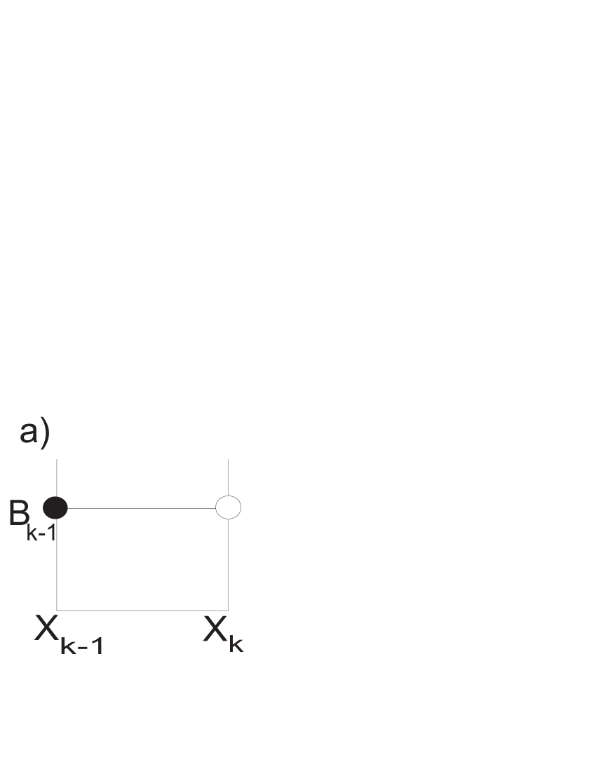
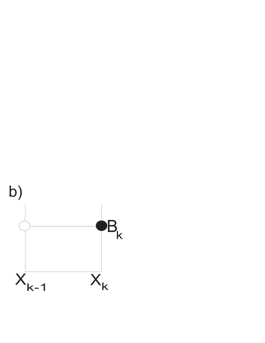
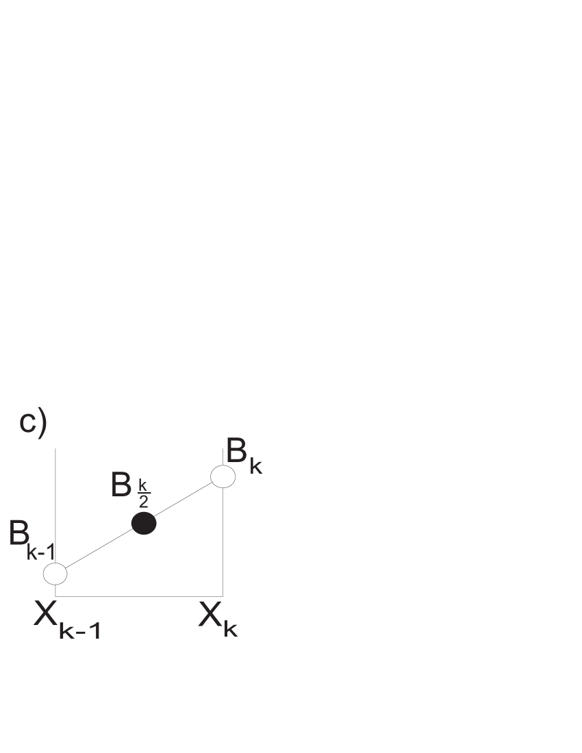
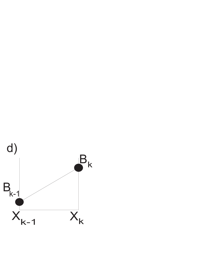
Figure 1:

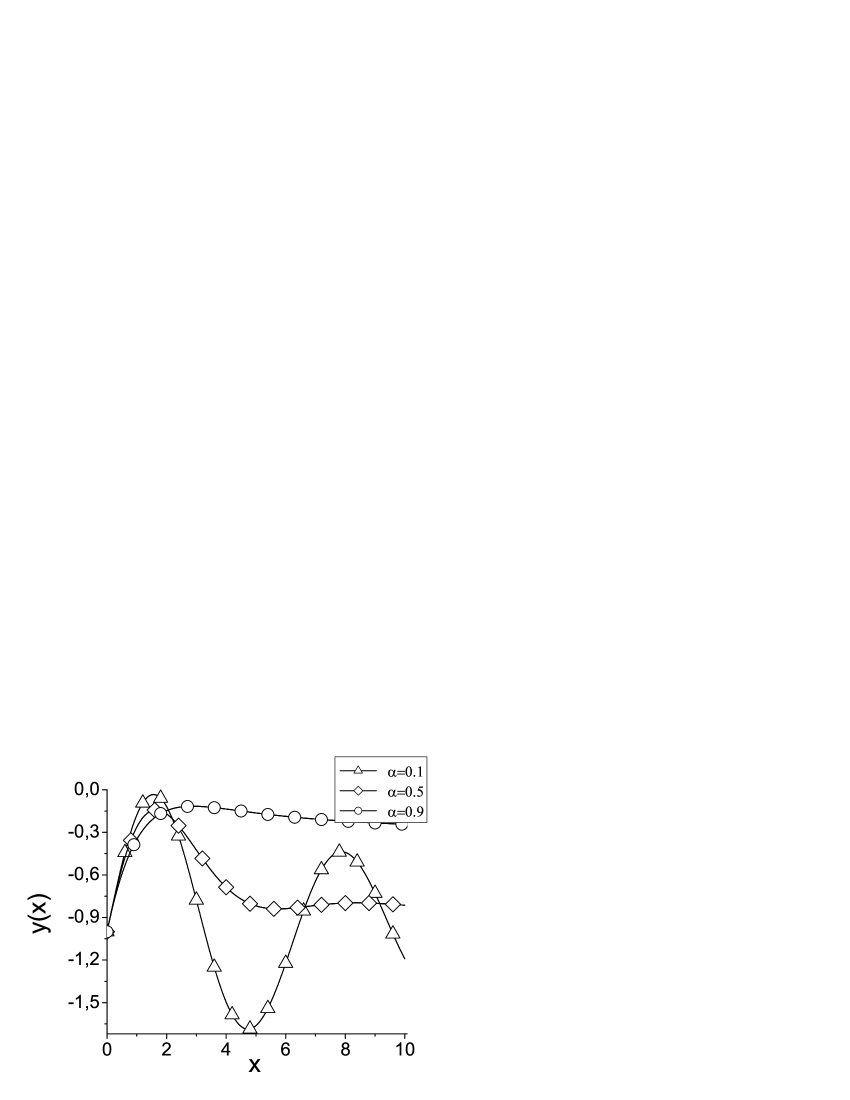
Figure 2:

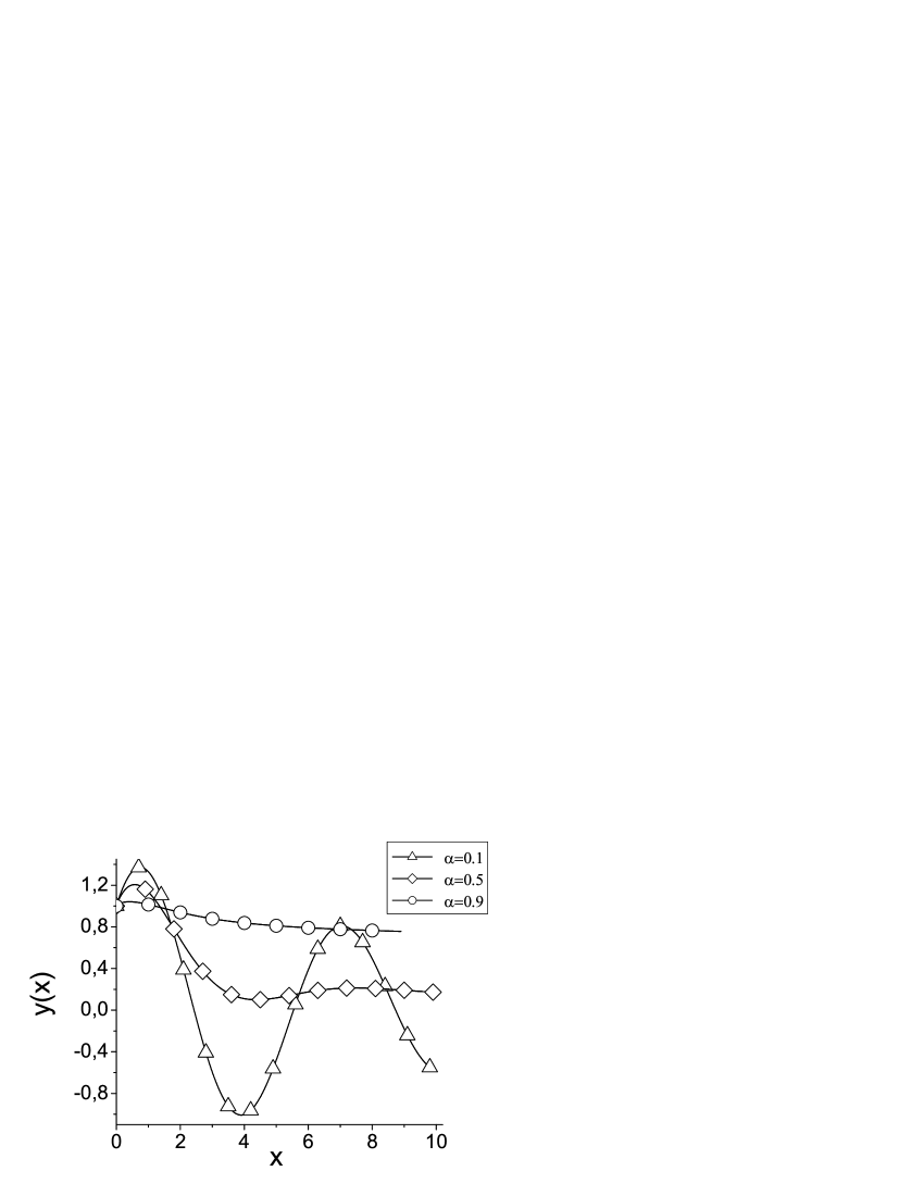
Figure 3:

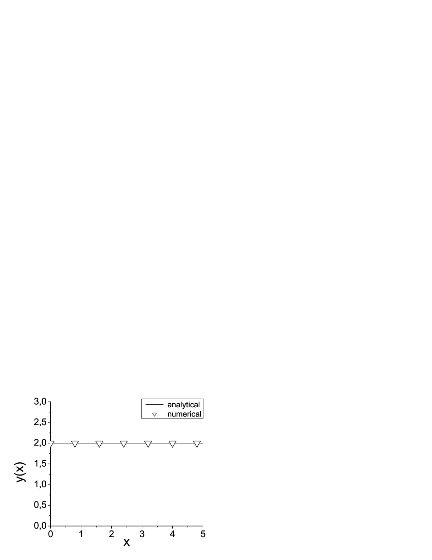
Figure 4:

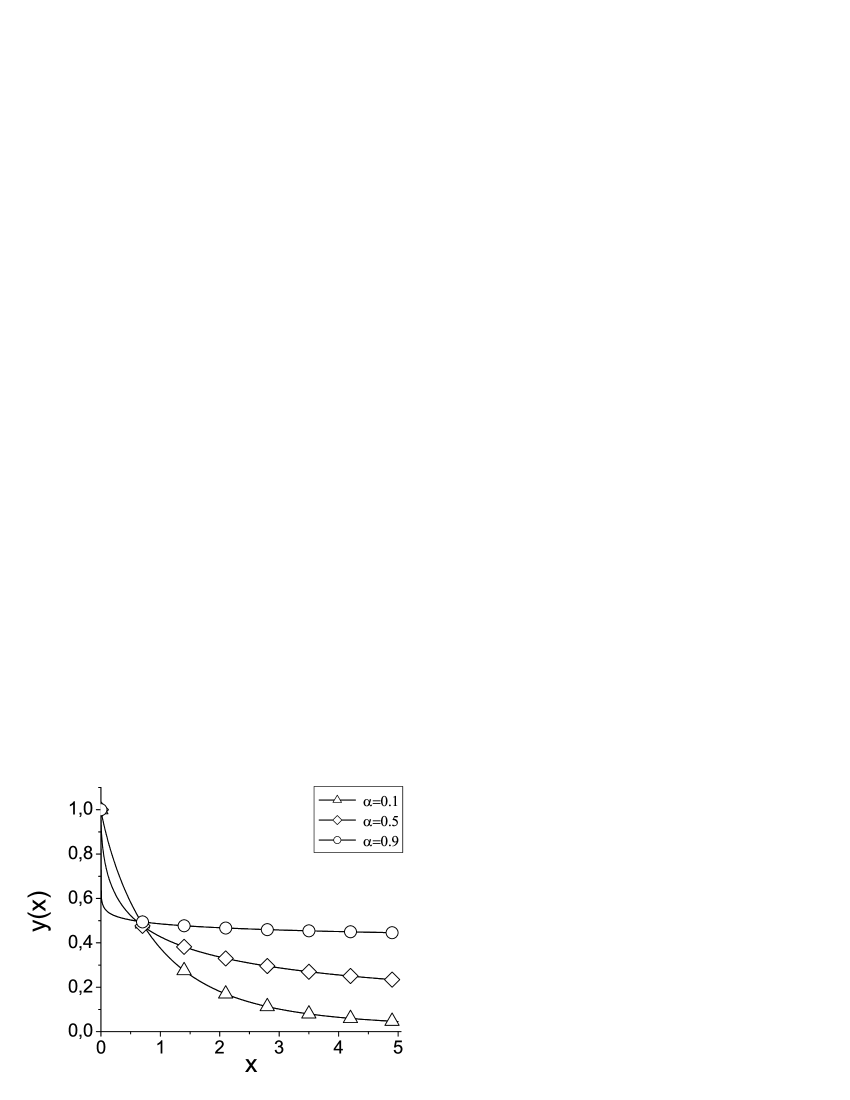
Figure 5:

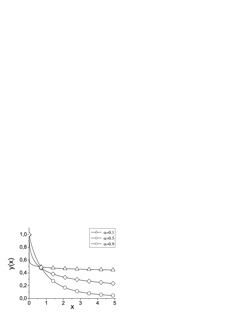
Figure 6:

List of captions for tables

• Analytical values of the Caputo derivative (52) and errors generated by discrete forms of the Caputo derivative (28) (29) (30) (31) for $h=0.01$.

• Analytical solution of Eqn. (7) with initial conditions (53) and errors generated by the Gear’s and Adams methods for $h=0.01$.

• Analytical results of Eqn. (7) with initial conditions (54) and errors generated by the Euler’s (algorithm 1.1), Adams (algorithm 1.2) and Gear’s (algorithm 1.3) methods for $h=0.01$.

• Analytical results of Eqn. (8) with initial conditions (55) and errors generated by the Euler’s (algorithm 2.1), Adams (algorithm 2.2) and Gear’s (algorithm 2.3) methods for $h=0.01$.

• Analytical results of Eqn. (10) with the initial condition $y(0)=1$ and errors generated by the Euler’s method (algorithm 4.1) for $h=0.01$.

• Analytical results of Eqn. (11) with the initial condition $y(0)=1$ and errors generated by the Euler’s method (algorithm 5.1) for $h=0.01$.

Table 1:

	$y\left(1\right)$	$y\left(4\right)$	$y\left(6\right)$	$y\left(8\right)$	$y\left(10\right)$
$\alpha=0.1$
analytical	1.0944780	15.2447755	32.9377877	56.8955141	86.9374806
errors generated by discrete forms of the Caputo derivative
case-I	1.04e-2	3.62e-2	5.22e-2	6.76e-2	8.26e-2
case-II	1.04e-2	3.62e-2	5.21e-2	6.75e-2	8.26e-2
case-III	1.77e-5	1.98e-5	2.02e-5	2.07e-5	2.10e-5
case-IV	0	0	2.00e-8	0	4.00e-8
$\alpha=0.5$
analytical	1.5045056	12.0360444	22.1116256	34.0430746	47.5766431
errors generated by discrete forms of the Caputo derivative
case-I	1.17e-2	2.30e-2	2.81e-2	3.24e-2	3.61e-2
case-II	1.08e-2	2.21e-2	2.72e-2	3.14e-2	3.52e-2
case-III	4.60e-4	4.64e-4	4.65e-4	4.66e-4	4.66e-4
case-IV	0	0	0	2.00e-8	1.00e-8
$\alpha=0.9$
analytical	1.9111582	8.7813771	13.7171223	18.8232939	24.0600562
errors generated by discrete forms of the Caputo derivative
case-I	1.60e-2	1.76e-2	1.81e-2	1.85e-2	1.88e-2
case-II	4.98e-3	6.54e-3	7.04e-3	7.41e-3	7.70e-3
case-III	5.53e-3	5.53e-3	5.53e-3	5.53e-3	5.53e-3
case-IV	0	0	0	1.00e-8	1.00e-8

Table 2:

	$y\left(1\right)$	$y\left(4\right)$	$y\left(6\right)$	$y\left(8\right)$	$y\left(10\right)$
$\alpha=0.1$
analytical	0.8226218	-0.4960927	-0.2222706	0.5587627	-0.1911696
errors generated by the Gear’s method
case-II	2.71e-4	1.39e-2	4.21e-3	5.77e-3	1.39e-2
case-III	1.40e-5	1.24e-5	4.23e-6	1.47e-5	7.66e-6
case-IV	1.06e-5	1.75e-5	3.08e-5	5.57e-6	3.18e-5
errors generated by the Adams method
case-II	8.55e-5	1.40e-2	4.27e-3	5.89e-3	1.40e-2
case-III	1.71e-4	1.05e-4	5.35e-5	1.11e-4	3.97e-5
case-IV	1.70e-4	1.14e-4	3.67e-5	1.09e-4	5.85e-5
$\alpha=0.5$
analytical	0.7374822	0.3129516	0.1623955	0.2017797	0.1867275
errors generated by the Gear’s method
case-II	7.85e-4	7.84e-3	5.76e-3	4.45e-3	5.04e-3
case-III	1.26e-4	1.02e-4	1.96e-5	2.53e-5	8.40e-6
case-IV	1.67e-4	7.25e-5	4.27e-5	4.71e-5	4.29e-5
error generated by the Adams method
case-II	6.92e-5	7.54e-3	5.62e-3	4.27e-3	4.87e-3
case-III	5.90e-4	3.97e-4	1.22e-4	1.56e-4	1.75e-4
case-IV	5.40e-4	2.22e-4	1.06e-4	1.34e-4	1.23e-4
$\alpha=0.9$
analytical	0.6512921	0.8643086	0.8128471	0.7787088	0.7563200
errors generated by the Gear’s method
case-II	2.29e-3	4.97e-3	5.13e-3	5.09e-3	5.06e-3
case-III	1.09e-3	5.18e-5	1.20e-4	7.50e-5	4.63e-5
case-IV	1.80e-3	2.39e-3	2.25e-3	2.15e-3	2.09e-3
errors generated by the Adams method
case-II	8.76e-5	1.78e-3	2.13e-3	2.23e-3	2.28e-3
case-III	1.25e-3	3.19e-3	3.06e-3	2.89e-3	2.78e-3
case-IV	5.65e-4	7.89e-4	7.37e-4	7.02e-4	6.79e-4

Table 3:

	$y\left(1\right)$	$y\left(4\right)$	$y\left(6\right)$	$y\left(8\right)$	$y\left(10\right)$
$\alpha=0.1$
analytical	-0.1773782	-1.4960927	-1.2222706	-0.4412373	-1.1911696
Euler	1.79e-5	2.68e-5	2.92e-5	4.23e-6	3.85e-5
Gear	1.40e-5	1.24e-5	4.18e-6	1.47e-5	7.60e-6
Adams	1.70e-4	1.14e-4	3.67e-5	1.09e-4	5.85e-5
$\alpha=0.5$
analytical	-0.2625177	-0.6870484	-0.8376044	-0.7982203	-0.8132725
Euler	1.26e-4	1.04e-4	2.41e-5	2.51e-5	9.32e-6
Gear	1.26e-4	1.02e-4	1.96e-5	2.53e-5	8.40e-6
Adams	5.40e-4	2.22e-4	1.06e-4	1.34e-4	1.23e-4
$\alpha=0.9$
analytical	-0.3487079	-0.1356914	-0.1871529	-0.2212912	-0.2436800
Euler	1.08e-3	5.29e-5	1.20e-4	7.49e-5	4.62e-5
Gear	1.06e-3	5.18e-5	1.20e-4	7.50e-5	4.63e-5
Adams	5.65e-4	7.89e-4	7.37e-4	7.02e-4	6.79e-4

Table 4:

	$y\left(1\right)$	$y\left(4\right)$	$y\left(6\right)$	$y\left(8\right)$	$y\left(10\right)$
$\alpha=0.1$
analytical	1.3290813	-1.0029826	0.3872104	0.4928008	-0.5873420
Euler	4.83e-3	3.40e-3	8.51e-4	3.06e-3	1.49e-3
Gear	4.83e-3	3.41e-3	8.92e-4	3.10e-3	1.49e-3
Adams	1.06e-2	6.39e-3	2.50e-3	7.28e-3	2.39e-3
$\alpha=0.5$
analytical	1.1341116	0.1100800	0.1748923	0.2090891	0.1714270
Euler	7.42e-3	8.06e-5	3.56e-4	8.41e-4	6.45e-4
Gear	7.42e-3	7.54e-5	3.53e-4	8.43e-4	6.45e-4
Adams	2.27e-2	7.88e-3	4.71e-3	6.06e-3	5.61e-3
$\alpha=0.9$
analytical	1.0146791	0.8374876	0.7913672	0.7652525	-
Euler	5.73e-3	2.17e-3	2.01e-3	1.96e-3	-
Gear	5.74e-3	2.17e-3	2.01e-3	1.96e-3	-
Adams	3.15e-2	3.69e-2	3.50e-2	3.37e-2	-

Table 5:

	$y\left(1\right)$	$y\left(2\right)$	$y\left(3\right)$	$y\left(4\right)$	$y\left(5\right)$
$\alpha=0.1$
analytical	0.3760660	0.1811155	0.1014866	0.0644356	0.0452231
Euler	1.36e-3	9.40e-4	5.42e-4	3.03e-4	1.70e-4
$\alpha=0.5$
analytical	0.4275836	0.3362040	0.2873412	0.2553957	0.2323262
Euler	9.61e-4	8.60e-4	7.88e-4	7.31e-4	6.85e-4
$\alpha=0.9$
analytical	0.4855645	0.4682030	0.4580801	0.4509182	0.4453768
Euler	1.23e-3	1.19e-3	1.17e-3	1.16e-3	1.14e-3

Table 6:

	$y\left(1\right)$	$y\left(2\right)$	$y\left(3\right)$	$y\left(4\right)$	$y\left(5\right)$
$\alpha=0.1$
analytical	0.4855645	0.4682030	0.4580801	0.4509182	0.4453768
Euler	1.33e-4	7.06e-5	4.85e-5	3.69e-5	3.07e-5
$\alpha=0.5$
analytical	0.4275836	0.3362040	0.2873412	0.2553957	0.2323262
Euler	8.39e-4	5.30e-4	3.73e-4	2.82e-4	2.23e-4
$\alpha=0.9$
analytical	0.3760660	0.1811155	0.1014866	0.0644356	0.0452231
Euler	1.55e-3	1.27e-3	7.99e-4	4.77e-4	2.88e-4

References

- [1] Blank, L.: Numerical treatment of differential equations of fractional order. Manchester Centre for Numerical Computational Mathematics, Numerical Analysis Report 287 (1996)
- [2] Caputo, M.: Linear models of dissipation whose Q is almost frequency independent, Part II. Geophys. J. R. Astr. Soc. 13, 529–539 (1967)
- [3] Caputo, M.: Models of flux in porous media with memory. Water Resource Res. 36, 693–705 (2000)
- [4] Diethelm, K.: An algorithm for the numerical solution of differential equations of fractional order. Elec. Transact. Numer. Anal. 5, 1–6 (1997)
- [5] Diethelm, K., Ford, N.J., Freed, A.D.: A predictor-corrector approach for the numerical solution of fractional differential equations. Nonlinear Dynamics 29, 3–22 (2002)
- [6] Diethelm, K., Ford, N.J., Freed, A.D: Detailed error analysis for a fractional Adams method. Numerical Algorithms 36, 31–52 2004
- [7] Diethelm, K., Ford, N.J., Freed, A.D, Luchko, Y.: Algorithms for the fractional calculus: A selection of numerical methods. Computer Methods in Applied Mechanics and Engineering 194, 743–773 (2005)
- [8] Diethelm, K., Luchko, Y.: Numerical solution of linear multi-term differential equations of fractional order. TU Braunschweig, Technical report (2001)
- [9] Ford, N.J., Connolly, J.A.: Comparison of numerical methods for fractional differential equations. CPAA 5, 289–307 (2006)
- [10] Galucio, A.C., Deü, J.-F., Mengué, S., Dubois, F.: An adaptation of the Gear scheme for fractional derivatives. Computer Methods in Applied Mechanics and Engineering 195, 6073–6085 (2006)
- [11] Gear, C.W.: Numerical initial value problems in ordinary differential equation. Prentice-Hall, Englewood Cliffs (1971)
- [12] Gorenflo, R., Luchko, Y., Mainardi, F.: Analytical properties and applications of the Wright function. Fractional Calculus and Applied Analysis 2, 383–414 (1999)
- [13] Gorenflo, R., Mainardi, F., Moretti, D., Pagnini, G., Paradisi P.: Discrete random walk models for space time fractional diffusion. Chemical Physics 284, 521–541 (2002)
- [14] Heymans N., Podlubny, I.: Physical interpretation of initial conditions for fractional differential equations with Riemann-Liouville fractional derivatives. Rheologica Acta 45, 765–771(7) (2006)
- [15] Hilfer, R.: Applications of Fractional Calculus in Physics. World Scientific, Singapore (2000)
- [16] Kilbas, A.A., Srivastava, H.M., Trujillo, J.J.: Theory and Applications of Fractional Differential Equations. Elsevier, Amsterdam (2006)
- [17] Leszczynski, J.S., Ciesielski, M.: A numerical method for solution of ordinary differential equations of fractional order. Lect. Notes in Comp. Sci. 2328, 695–702 (2002)
- [18] Leszczynski, J.S.: Using the fractional interaction law to model the impact dynamics of multiparticle collisions in arbitrary form. Phys. Rev. E 70, 51315-1–051315-15 (2004)
- [19] Mainardi, F., Raberto, M., Gorenflo, R., Scalas, E.: Fractional calculus and continuous-time finance II: the waiting-time distribution. Physica A 287, 468–481 (2000)
- [20] Miller, K.S., Ross, B.: An introduction to the fractional differential equations. Wiley and Sons, New York (1993)
- [21] Oldham, K.B., Spanier, J.: The fractional calculus. Theory and applications of differentiation and integration to arbitrary order. Academic Press, New York (1974)
- [22] Palczewski, A.: Ordinary differential equations: theory and numerical methods (in Polish). WNT, Warsaw (1999)
- [23] Podlubny, I.: Fractional Differential Equations. Academic Press, San Diego (1999)
- [24] El-Sayed, A.M.A., El-Mesiry, A.E.M., El-Saka, H.A.A.:Numerical solution for multi-term fractional (arbitrary) orders differential equations. Computational and Applied Mathematics 23, 33–54 (2004)
- [25] Samko, S.G., Kilbas, A.A., Marichev, O.I.: Fractional Integrals and Derivatives. Theory and Applications. Gordon and Breach, Amsterdam (1993)
- [26] Scalas, E., Gorenflo, R., Mainardi, F.: Fractional calculus and continuous time finance. Physica A 284, 376–384 (2000)
- [27] Schumer, R., Benson, D.A., Meerschaert, M.M., Wheatcraft, S.W.: Eulerian derivation of the fractional advection dispersion equation. J. Contaminant Hydrol. 48, 69–88 (2001)
- [28] Zaslavsky, G.: Hamiltonian Chaos and Fractional Dynamics. Oxford University Press, Oxford (2005)