A Non-linear Generalization of Singular Value Decomposition
and its Application to Cryptanalysis

Abstract

Singular Value Decomposition (SVD) is a powerful tool in linear algebra and has been extensively applied to Signal Processing, Statistical Analysis and Mathematical Modeling. We propose an extension of SVD for both the qualitative detection and quantitative determination of nonlinearity in a time series. The paper illustrates nonlinear SVD with the help of data generated from nonlinear maps and flows (differential equations). The method is to augment the embedding matrix with additional nonlinear columns derived from the initial embedding vectors and extract the nonlinear relationship using SVD. The paper also demonstrates an application of nonlinear SVD to cryptanalysis where the encrypted signal is generated by a nonlinear transformation. A comparison of the method for both noise-free and noisy data along with their surrogate counterparts is included.

Singular Value Decomposition (SVD) along with its related variation known as Principal Component Analysis is a powerful technique for data analysis in linear algebra which has found lot of applications in various fields such as Signal Processing, Statistical Analysis, Biomedical Engineering , Genetics Analysis, Mathematical and Statistical Models, Graph Theory, Psychology etc Intro . In this paper, we discuss an extension of SVD for both the qualitative detection and quantitative determination of nonlinearity in a time series. SVD is performed on the embedding matrix created from data series. The conventional SVD can determine the form of linear relationships among data vectors. For the proposed method, the embedding matrix is augmented by nonlinear columns derived from the usual ones. Now if the SVD gives zero singular values there is a linear relationship present among the columns. In that case, we could exactly determine the nonlinearity present in the data. The paper also demonstrates an application of nonlinear SVD to cryptanalysis where the encrypted signal is generated by a nonlinear transformation. Nonlinear methods are useful in cryptography as the signals to be decrypted are often generated by non-linear transformations. We have included examples of maps (Logistic map and Henon map) and flows (Van der Pol oscillator and Duffing oscillator) to illustrate the method of nonlinear SVD to identify parameters. The paper presents the recovery of parameters in the following scenarios: (i) data generated by maps and flows (ii) Comparison of the method for both noisy and noise-free data (iii) Surrogate data Analysis for both the noisy and noise-free cases

I Introduction

Historically SVD has been used for finding the dimension of a linear system as it gives statistically independent set of variables which could span the state space. Standard SVD based methods known as Singular Spectrum Analysis were used for detecting nonlinearity in a qualitative manner  broomhead . An abrupt decrease in the profile of the singular spectrum is an indication of lower dimensional determinism. But this method fails to distinguish between a chaotic data and its surrogates  Sahay ; Abarbanel . The failure of this method for some well known chaotic processes, and when the data is corrupted with noise are also reported  Kugiumtzis ; Buzug . Bhattacharya and kanjilal proposed a method of quadratic scaling of singular values in order to detect the determinism in time series Bhattacharya . The decreasing singular values were weighted more to highlight the deterministic and stochastic features. This method could qualitatively distinguish between the data series and its surrogates.

The Grassberger- Procaccia (G - P) algorithm was used to show that a finite correlation dimension of an irregular time series is an indication of underlying deterministic nonlinearity Grassberger . G - P algorithm has a few drawbacks as it fails when the data is noisy and is unable to distinguish stochastic processes with power-law power-spectra from chaos Osborne ; Ruelle . There are various methods to detect the underlying determinism in a time series. One uses the distribution of correlation coefficients as a qualitative method to distinguish chaos from noise because the spectrum is flat for noise but gradually decays for chaos Sugihara . But this method fails to distinguish between correlated noise and chaos Cazellus ; Ensminger . Similarly in Statistics, the distribution of sample autocorrelation function (ACF) is used as an important tool to assess the degree of dependance in data in order to select a model  statistics text book . A constant sample ACF, which takes zero values for all the lags (delays) is an indication of data being independent and identically distributed (iid) noise. If the sample ACF spectrum shows decay or oscillations appropriate statistical parametric models could be used to model the data. There are developments in the field of both linear and nonlinear versions of Autoregressive(AR) and Autoregressive Moving Average(ARMA) models along with many robust algorithms; e. g. the Fast Orthogonal Search method which can obtain correct model parameters irrespective of the model selection  Korenberg .

If one is interested in a detection of the existence of nonlinearity but not the determination of the underlying model A. Porta et. al. suggest an alternate method  porta1 ; porta2 . Their method consists of using Takens embedding of data in a higher dimensional phase space and then subdividing the phase space into non-overlapping hypercubes. Prediction is based on the behavior of the median member of each hypercube. They find that an error function dips much further with actual data than with its surrogates.

Linear and nonlinear AR and ARMA models are efficiently used for determining the nonlinearity; i.e. to find the parameters of the appropriate models using optimal parameter search (OPS) algorithms  Sheng Lu and through various least square techniques: Least Square strang , Total Least Square TLS and Minimizing the Hypersurface Distance Sheng Lu2 . In this paper, we discuss a nonlinear extension of SVD to detect and exactly determine the nonlinearity with an application to cryptography. The proposed method of nonlinear SVD for maps is similar to the nonlinear AR and ARMA regression proposed by Lu. S et al Sheng Lu and Marmarelis  Marmarelis . But the method is not limited to polynomial regression. Any deterministic nonlinearity present in the data could possibly be recovered. Nonlinear SVD method could be considered as functional regression in an extended phase space.

Chaotic cryptanalysis is an emerging field of chaotic cryptography which deals with the breaking of secret codes without any access to the super keys or parameters of the system  PGV ; PGV-a ; PGV-b . It often deals with the problem of system identification from the encrypted data which could be noisy and incomplete. Consider two parties communicating across a private channel. The aim of cryptanalysis is to decrypt the message. The signal sent across the channel looks random but it is generated by a deterministic dynamical system. Since the intended recipient has some information about the system parameters (a key) she can retrieve the information from the encrypted signal. All that the cryptanalyst knows about the signal is that it must have been generated by a deterministic dynamical system. He has no clue about the parameters or the dimension of the system. Here we are proposing a new cryptanalysis tool based on SVD to find the information about a system from the encrypted signal. Nonlinear SVD and time delayed embedding together with the method of finding derivatives from data  PGV1 can be used to identify the nonlinearity of the system from the time series.

The paper is organized as follows. Section I is introduction. Section II briefly reviews the conventional SVD technique. Section III describes the method of nonlinear SVD and Section IV discuss the applicability of the method to data series. A numerical example of retrieval of Logistic map parameter from data is discussed in Section V. Section VI gives the comparison of nonlinear SVD and conventional SVD analysis of the data and its surrogates. Section VII discusses the extension of the method for higher order maps. Section VIII shows the numerical results in the presence of two types of noises: Uniform noise and Gaussian noise. Section IX is the extension of the method to flows and recovery of the nonlinearity from chaotic data is explained in Section X. Section XI is a discussion on linear and nonlinear models. Section XII is discussion on cryptanalysis and the conclusions is Section XIII.

II Singular Value Decomposition

Singular Value Decomposition can be considered as a generalization of the spectral-decomposition of square matrices, to analyze rectangular matrices. SVD decomposes a rectangular matrix into three simple matrices: two orthogonal matrices and one diagonal matrix  strang . In general, SVD theorem can be stated as follows: any $m\times n$ matrix $A$, with $m\geq n$ can be factored into three matrices: $U$ (column orthogonal, $m\times n$ matrix), $W$ (diagonal,$n\times n$ matrix) and $V$ (orthogonal $n\times n$ matrix). When $A$ is real, $A=U.W.V^{T}$ (where $V^{T}$ is the transpose of $V$). For complex matrices, $W$ remains real but $U$ and $V$ become unitary. The diagonal elements of $W$ matrix are known as the singular values of $A$.

This decomposition is a technique that works well with matrices that are either singular or else numerically very close to singular. SVD is also used to calculate pseudo-inverses when the natural inverse of the matrix does not exist  N.Recipe . SVD and pseudo-inverses are generally used in statistics for solving least square problems. Data compression using SVD is one of the standard applications in image processing  strang ; kalman .

III Method of Nonlinear Singular Value Decomposition

Given a time series generated by any system $\{X\}=\{X_{1},X_{2},X_{3},\ldots,X_{N}\}$ the aim of nonlinear system identification is (i) to detect if there is nonlinearity and (ii) to exactly determine the equation which generated the data. The current study is based on the data generated by nonlinear maps and flows. We will begin by using the standard Takens embedding: a method of reconstruction of the state space with time delayed data segments known as embedding vectors  Takens . The embedding matrix $E$ is created from the time delayed vectors as follows. A typical embedding vector $Y^{i}$ is the $m$ dimensional embedding vector generated from the given time series.

$$Y^{1} = (X_{1}\ X_{2}\ldots X_{m}\ )^{T}.$$

$$Y^{2} = (X_{2}\ X_{3}\ldots X_{m+1}\ )^{T}.$$

$$\ldots$$

$$Y^{i} = (X_{i}\ X_{i+1}\ldots X_{m+i}\ )^{T}.$$

Note that $(X_{1}\ X_{2}\ldots X_{m}\ )^{T}$ is a column vector and denotes the transpose of $(X_{1}\ X_{2}\ldots X_{m}\ )$. The collection $\{Y^{i}\}$ is the time delay embedding of the given data. Let the embedding matrix $E$ be created from $k$ embedding vectors as follows.

$$E=\left[\small\begin{array}[]{cccccc}&(Y^{1})^{T}\\ &(Y^{2})^{T}\\ &\ldots\\ &\ldots\\ &\\ &(Y^{k})^{T}\\ \end{array}\right]=\left[\small\begin{array}[]{cccccc}X_{1}&X_{2}&&\ldots&&X_{m}\\ X_{2}&X_{3}&&\ldots&&X_{m+1}\\ &&&\ldots&&\\ X_{k}&X_{k+1}&&\ldots&&X_{m+k}\\ \end{array}\right].$$ (1)

For nonlinear SVD, we extend the embedding matrix $E$ by adding nonlinear columns. Let F be the extended embedding matrix.

$$F=[E\ :\ f_{1}\ f_{2}\ \ldots f_{i}\ ]$$ (2)

The last $i$ columns of $F$ matrix, $f_{1},f_{2}\ldots f_{i}$ are functions of the columns of $E$ matrix, $\{E^{<1>},E^{<2>}\ldots E^{<m>}\}$ where $E^{<i>}$ denotes the $i^{th}$ column of $E$. In general, a non-linear column refers to the square, cube, any other higher powers of a column, the product of two or more columns or any other kind of non-linearity such as exponentiation and trigonometric functions of the column. If there is a non-linear relationship between the time delayed vectors, it could be interpreted as a linear relationship between the time-delayed vectors and corresponding nonlinear columns. The dimension of $F$ matrix is $k\times p$ where $p=(m+i)$. This extended embedding matrix can be considered as a higher dimensional linear system. The singular value decomposition can find the linear relation between the embedding vectors and corresponding nonlinear columns, thus recovering the nonlinear relationship inherent in the data. SVD is performed on F to get,

$$\ \ F=UWV^{T}.$$ (3)

Therefore,

$$FV=UW.$$ (4)

Expanding Eq. 4

$$F.\left[\small\begin{array}[]{cccccc}V^{<1>}&V^{<2>}&\ldots&V^{<p>}\\ \end{array}\right]=\left[\small\begin{array}[]{cccccc}U^{<1>}&U^{<2>}&\ldots&U^{<p>}\\ \end{array}\right].\left[\small\begin{array}[]{cccccc}W_{1,1}&0&0&\ldots&0\\ 0&W_{2,2}&0&\ldots&0\\ 0&0&&\ldots&\ldots\\ 0&\ldots&&\ldots&W_{p,p}\\ \end{array}\right]$$ (5)

Using partitions of $V$ and $W$ and expanding along the last column of $V$ and $W$ we get,

$$\left[\small\begin{array}[]{cccccc}F^{<1>}&F^{<2>}&\ldots&F^{<p>}\\ \end{array}\right].\left[\small\begin{array}[]{cccccc}&V_{1,p}\\ &V_{2,p}\\ &\ldots\\ &V_{p,p}\\ \end{array}\right]=\left[\small\begin{array}[]{cccccc}U^{<1>}&U^{<2>}&\ldots&U^{<p>}\\ \end{array}\right].\left[\small\begin{array}[]{cccccc}&0\\ &0\\ &\ldots\\ &W_{p,p}\\ \end{array}\right].$$ (6)

$$V_{1,p}(F^{<1>})+V_{2,p}(F^{<2>})+\ldots+V_{p,p}(F^{<p>})=0(U^{<1>})+0(U^{<2>})+\ldots+W_{p,p}(U^{<p>})$$ (7)

(Note that $U^{<i>}$ stands for the $i^{th}$ column of $U$ matrix. $W_{i,j}$ is the element on $i^{th}$ row and $j^{th}$ column of $W$ matrix). If the $p^{th}$ singular value of W is zero,

$$W_{p,p}=0.$$

then

$$V_{1,p}(F^{<1>})+V_{2,p}(F^{<2>})+\ldots+V_{p,p}(F^{<p>})=0.$$ (8)

Or, in another notation,

$$\sum_{p}{F_{j,p}.V_{p,n}}=0\ \ \ \forall\ j$$ (9)

Eq. 8 and 9 can be seen as a statement that the columns of $F$ including those formed by the nonlinear functions $\{f_{1},f_{2}\ldots f_{i}\}$ now span a linear vector space. This equation is true for all rows of $F$ and hence by exploiting this relation, the dependance between the linear and nonlinear columns of the $F$ matrix can be recovered.

IV Nonlinear SVD of data

We begin with our assumption that the underlying equation is a function of the delay vectors. In case the data is noise free and the conventional SVD of data does not result in a small enough singular value then we try different $F$’s of the form $F=[E\ :\ f_{1}\ f_{2}\ \ldots f_{i}\ ]$ as shown in Section III. We keep trying different $f_{i}$’s till the nonlinear SVD gives at least one nearly zero singular value. Next section shows a numerical example of data generated by Logistic map. We made a simple guess for the nonlinear function and it worked for that case. If it did not,we would have tried other functions.

But when the data is noisy, the singular value $W_{p,p}\neq 0$ even if we get the right $F$ matrix of nonlinear functions. Hence we try different nonlinear functions and choose the $F$ that gives the lowest value of $W_{p,p}$. Ideally we want $\frac{W_{p,p}}{W_{1,1}}$ (the ratio of $p^{th}$ singular value to the $1^{st}$ singular value) to be below some preset criterion. As the noise level in the data increases chances are higher that the method of nonlinear SVD fails. Therefore our confidence in the estimated model equation goes down with the increase in noise.

V Numerical Example

Consider the data generated by a Logistic map $X_{n+1}=\lambda.X_{n}.(1-X_{n})$ where $0\leq X<1$ and $\lambda$ is an unknown parameter. We show in this section how $\lambda$ could be retrieved from the data. Let the data series sampled at a chosen time delay $\tau$ be $\{X_{n}\}={\{X_{1},X_{2},\ldots,X_{N}}\}$. The data can be embedded in three dimensions using embedding vectors as shown in the following matrix :

$$E=\left[\small\begin{array}[]{cccccc}X_{1}&X_{2}&X_{3}\\ X_{2}&X_{3}&X_{4}\\ &\ldots&\\ X_{5}&X_{6}&X_{7}.\end{array}\right].$$

The dimension of $E$ matrix is $5\times 3$. After SVD operation on the embedding matrix $E$, we observed that none of the singular values of $E$ go to zero indicating no linear dependance present in the data. Now $E$ matrix is extended to $F$ matrix as follows,

$$F = [E\ :\ f_{1}\ ]$$

$$= [E^{<1>}\ E^{<2>}\ E^{<3>}\ f_{1}\ ]$$

$$= [E^{<1>}\ E^{<2>}\ E^{<3>}\ {E^{<1>}}^{2}\ ]$$

So that a typical row of $F$ is seen as $[\ X_{p}\ X_{p+1}\ X_{p+2}\ {X_{p}}^{2}\ ]$ where $p$ goes from $1$ to $4$. SVD of $F$ gives a zero singular value $W_{4,4}=0$ indicating a linear dependence between the first column $X_{n}$ and the added nonlinear column ${X_{n}}^{2}$. Eq. 8 for this particular numerical example is,

$$V_{1,4}(X_{n})+V_{2,4}(X_{n+1})+V_{3,4}(X_{n+2})+V_{4,4}(X_{n}^{2})=0.$$ (10)

Substituting the numerical values, the exact equation can be recovered from Eq. 9 as follows.

$$-0.696311X_{n}+0.174078X_{n+1}+0X_{n+2}+0.696311X_{n}^{2} = 0.$$

$$4X_{n}-X_{n+1}-4{X_{n}}^{2} = 0.$$

$$4{X_{n}}(1-{X_{n}}) = X_{n+1}.$$

For the numerical example, the initial condition that generated the trajectory was $0.02$ and the selected parameter value $\lambda$ of the logistic map was $4$. We have observed that the method of nonlinear SVD works reasonably well even in the presence of noise, provided the noise is below some threshold value. Let the data $\{X_{n}\}$ be contaminated by additive noise $\{P_{n}\}$ which is either gaussian or uniform, $\{\widehat{X}_{n}\}=\{X_{n}\}+\{P_{n}\}.$ The same procedure can be done on the embedding matrix $F$ created from the noisy data $\{{\widehat{X}_{n}}\}$ to extract the nonlinearity. TABLE. 1 shows the estimated values of parameter $\lambda$ for the data generated by Logistic family of maps under the presence of different types of noises. The preset criterion for the noisy case was $10^{-6}$. For recovering the parameters, we made an assumption that the singular values smaller than this can be considered zero and the underlying equation is extracted as explained in the noise-free case.

VI Comparison of Non-linear SVD with standard SVD and Surrogates

Fig. 1 shows the quadratically scaled singular value spectrum: $n^{2}.\sigma_{n}$ versus $n$; where $\sigma_{n}$ is the $n^{th}$ singular value generated by the standard SVD on the embedding matrix $E$. The time series $\{X\}$ generated from the Logistic map: $X_{n+1}=\lambda X_{n}(1-X_{n})$ where $0\leq X_{n}\leq 1$ and $\lambda=4$ is used to create an embedding matrix $E$ with unity delay as explained in section III. The dimension of the embedding matrix is selected as $21\times 21$ for this particular example. Standard SVD operation gives 21 non-zero singular values: Note that the profile gradually increases and slowly comes down. Similarly for the nonlinear SVD operation, the embedding matrix $F$ is generated as explained in section IV. The dimension of the embedding matrix is kept same as that of $E$ i.e. $21\times 21$ of which the last 10 columns are squares of the first 10 columns. Now SVD operation gives 21 singular values, out of which the last 10 are zero. Observe that the nonlinear SVD profile is significantly different from that of conventional SVD case as the former is ‘flat’ towards the end. Fig. 1, the spectrum for nonlinear SVD shows zero singular values compared to the standard SVD. There is a significant qualitative change in the spectrum. The profile of nonlinear SVD case drops to zero rapidly compared to the standard SVD case.

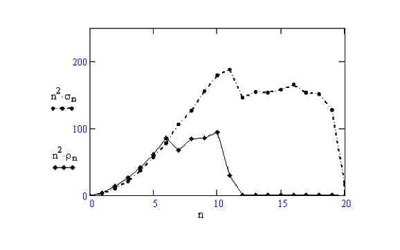
Figure 1: quadratically scaled spectrum of singular values for the case of standard SVD $(n^{2}.\sigma_{n})$ and non-linear SVD $(n^{2}.\rho_{n})$.

Similar analysis is done for the surrogates. Surrogates are generated from the Fourier Transform of the data by randomizing the phases. K surrogate data series $\{Xsurr(k)\}$ are generated from $\{X\}$ such that $\{Xsurr(k)\}$ and $\{X\}$ have the same power spectrum  Theiler Kennel . Hence $\{Xsurr(k)\}$ is considered as the nondeterministic counterpart of $\{X\}$ . Fig. 2 (i) and (ii) show the quadratically scaled spectra of singular values of the data and its surrogates for the standard SVD and nonlinear SVD respectively under noise free conditions. We observe that the selection of nonlinear columns has worked since the nonlinear SVD has given identically zero singular values as shown (ii) of Fig. 2. Moreover the method is able to clearly distinguish between the data and the surrogates. The figures also contain the spectrum for the original data $\{X\}$ for a comparison with its surrogates. Similar analysis for noisy data is included in section VIII.

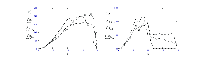
Figure 2: (i) Quadratically scaled spectrum of singular values by standard SVD on the data $(n^{2}.\sigma_{n})$ and its surrogates $(n^{2}.\sigma_{S1_{n}})$ and $(n^{2}.\sigma_{S2_{n}})$. (ii) Similar spectrum by nonlinear SVD for the data $(n^{2}.\rho_{n})$ and its surrogates $(n^{2}.\rho_{S1_{n}})$ and $(n^{2}.\rho_{S2_{n}})$.

Assume that we have varied the number and types of the nonlinear terms present in the embedding matrix $F$. For the case of data from quadratic map, we have added cubic columns in the F matrix instead of quadratic columns. The singular value spectrum looks qualitatively the similar to the quadratic case as shown in Fig. 3. But the exact relationship cannot be retrieved quantitatively, as none of the singular values go to zero. We need to try different embedding matrices and select the one which gives at least one nearly zero singular value.

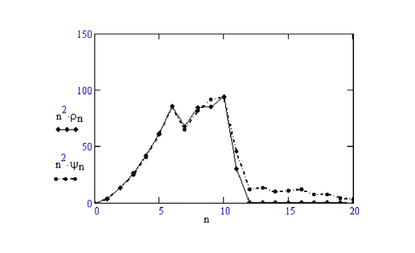
Figure 3: quadratically scaled singular value spectra by nonlinear SVD for different choices of $F$ matrices on data generated by Logistic map(i) $n^{2}.\rho_{n}$ versus $n$ ; where $\rho_{n}$ is the $n^{th}$ singular value of $F$ with quadratic columns, and (ii) $n^{2}.\phi_{n}$ versus $n$ ; where $\phi_{n}$ is the $n^{th}$ singular value of $F$ with cubic columns

VII Recovering non-linearity: Higher order maps

Let us now discuss the problem of recovering the non-linear equation when the data is generated from a higher order map of the following form,

$$X_{n+2}=f(X_{n},X_{n+1}).$$ (11)

The well known Henon map, falls in this category.

$$X_{n+1} = c-aX_{n}^{2}+Y_{n}.$$ (12)

$$Y_{n+1} = bX_{n}.$$ (13)

We generated some data using this map and later assumed that only the $X$ data is available. In that case it is more convenient to list this in the form of Eq. 11. With that form in mind we set up F to be ${[\ 1\ X_{n+2}\ X_{n+1}\ X_{n}\ {X_{n}}^{2}\ X_{n+1}^{2}\ (X_{n+1}X_{n})\ ]}$. Performing SVD on the embedding matrix $F$ we get the following relationship between the iterates.

$$0 = 0.496904-0.6956656X_{n+1}^{2}+0.1490712X_{n}-0.496904{X_{n+2}}.$$

$$0 = 1-1.4X_{n+1}^{2}+0.3X_{n}-{X_{n+2}}.$$

Therefore,

$${X_{n+2}}=1-1.4X_{n+1}^{2}+0.3X_{n}.$$ (14)

This can be seen as equivalent to Eq. 12 and 13 with parameter values $a=1.4\ b=0.3$ and $c=1$. Thus using the proposed method the parameters are retrieved from the X data.

Similarly Consider the case of the Logistic map again. We are once again required to find the parameters $\lambda$, but all the od iterates of the time series are suppressed. In this case we could consider the map of the form,

$$X_{n+2}=g(X_{n}).$$ (15)

The non-linear SVD on the modified data can retrieve a quartic nonlinearity. The predicted equation, for this particular example is of the form $g(x)=Bx+Cx^{2}+Dx^{3}+Ex^{4}$ where $B,C,D,E$ are functions of the parameter $\lambda$. SVD on $F=[\ X_{n}\ X_{n+2}\ {X_{n}}^{2}\ {X_{n}}^{3}\ {X_{n}}^{4}]$ gives a zero singular value corresponding to the following relationship between the columns.

$$0=14.7609X_{n}-X_{n+2}-71.4725{X_{n}}^{2}+113.4232{X_{n}}^{3}-56.7116{X_{n}}^{4}.$$

Therefore,

$$X_{n+2}=14.7609X_{n}-71.4725{X_{n}}^{2}+113.4232{X_{n}}^{3}-56.7116{X_{n}}^{4}.$$ (16)

But for the Logistic map $X_{n+1}=\lambda X_{n}(1-X_{n})$. Hence the second iterate can be written as a function of its first iterate as follows,

$$X_{n+2}=(\lambda^{2})X_{n}-(\lambda^{2}+\lambda^{3}){X_{n}}^{2}+(2\lambda^{3}){X_{n}}^{3}-(\lambda^{3}){X_{n}}^{4}.$$ (17)

Comparing Eq. $16$ and $17$ we recover the value of the parameter $\lambda=3.842$.

VIII Numerical results for noisy data

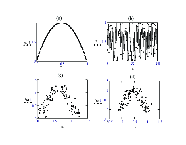
Figure 4: Time series (a) the chaotic data generated from the Logistic map: $X\mapsto 4X(1-X)$ where $0\leq X\leq 1$ (b) The phase space. (c) Phase space for noisy data (added uniform noise N(0,1)with noise level 28.089 %) (d) Phase space for noisy data (added gaussian noise N(0,1)with noise level 28.123 %). Noise level is defined as the ratio of the maximum noise value to the maximum signal value.

Fig. 3 (c) and (d) show the state space created from the noisy data for both the uniform and gaussian noises. Conventional SVD on the noisy data gives the value of $W_{p,p}/W_{1,1}$ somewhere in the range $(10^{-1},10^{-3})$ for different noise levels of the data from Logistic and Henon Maps shown in TABLE I and II. For nonlinear SVD, we have set value of the criterion $\frac{W_{p,p}}{W_{1,1}}$ as $10^{-6}$. If the ratio $\frac{W_{p,p}}{W_{1,1}}$ is below the preset value $10^{-6}$ the parameters are retrieved from the data. As the noise increases the method almost breaks down and even fails to distinguish between the data and its surrogates.

We found that when the noise level was low, the non-linear SVD was able to recover the non-linearity. TABLE. 1 shows the estimated values of parameter $\hat{a},\hat{b}$ for the data generated by Logistic family of maps: $X_{n+1}=a_{1}X_{n}-a_{2}{X_{n}}^{2}$ where $0\leq X_{n}\leq 1$ for the values of $a=4$ and $b=4$ for different Peak Signal to Noise Ratio (PSNR) using the nonlinear SVD algorithm. PSNR is defined as $20.\log\{\max(\textrm{Signal})/\sqrt{MSE}\}$ where MSE is the Mean Squared Error, the average of the square of the noise added to the signal. The proposed method works well when the PSNR is above $28$ for Gaussian noise and $33$ for Uniform noise. It seems that the method breaks down as the noise content in the signal increases (i.e. for lower PSNR values). Similarly Table. II shows the estimated values for parameter $\hat{a},\hat{b},\hat{c}$ for the Henon map ${X_{n+1}=c-aX_{n}^{2}+Y_{n};\ Y_{n+1}=bX_{n}}$ in the presence of noise using nonlinear SVD. Again the method breaks down for higher noise contents (PSNR $<30$) as we saw in the Logistic case.

Table 1: Estimated values of estimates $\hat{a_{1}},\hat{a_{2}}$ for the Logistic map: $X_{n+1}=a_{1}X_{n}-a_{2}{X_{n}}^{2}$ where $0\leq X_{n}\leq 1$ for the parameter values $a_{1}=4$ and $a_{2}=4$ in the presence of noise using nonlinear SVD. Peak Signal to Noise Ratio (PSNR) defined as $20.\log\{\max(\textrm{Signal})/\sqrt{MSE}\}$.

Parameters	Noise (Uniform Distribution)			Noise (Gaussian Distribution)
	$\hat{a_{1}}$	$\hat{a_{2}}$	PSNR	$\hat{a_{1}}$	$\hat{a_{2}}$	PSNR
	4.0367	3.9941	44.2314	4.099	4.0879	43.4502
$a_{1}$ = 4	4.1427	4.0206	38.7308	4.106	4.0919	41.8398
$a_{2}$ = 4	3.8757	3.8473	37.7963	4.247	4.1568	37.095
	4.2358	4.1516	36.4626	4.299	4.1484	34.5231
	4.3895	4.2506	33.6095	4.1563	3.9952	32.8561
	4.4809	4.2783	30.7117	4.0301	3.824	28.8170
	4.429	3.8507	24.6316	3.8041	2.5627	24.151

Table 2: Estimated values of parameters $\hat{a},\hat{b},\hat{c}$ for the Henon map ${X_{n+1}=c-aX_{n}^{2}+Y_{n};\ Y_{n+1}=bX_{n}}$ in the presence of noise using nonlinear SVD.

Parameters	Noise (Uniform Distribution)				Noise (Gaussian Distribution)
	$\hat{a}$	$\hat{b}$	$\hat{c}$	PSNR	$\hat{a}$	$\hat{b}$	$\hat{c}$	PSNR
	1.389	0.2896	1.003	46.863	1.4001	0.2998	1.003	44.5158
a = 1.4	1.3812	0.2923	1.010	40.764	1.3983	0.2964	1.005	40.93
b = 0.3	1.357	0.2769	1.009	36.178	1.4	0.3167	0.9881	35.93
c = 1.0	1.3717	0.262	1.0204	32.975	1.4376	0.3258	1.008	34.113
	1.3665	0.2758	1.067	30.4932	1.396	0.3279	1.04	31.336
	1.2969	0.2680	1.0349	26.549	1.5206	0.3401	1.08	28.3245
	1.3268	0.1566	1.1489	20.8353	1.2512	0.2917	0.9547	22.714

Fig. 4 shows the quadratically scaled singular spectra by standard SVD on the logistic data $(n^{2}.\sigma_{n})$ and its surrogates $(n^{2}.\sigma_{S1_{n}})$ and $(n^{2}.\sigma_{S2_{n}})$ along with similar spectrum by nonlinear SVD for the data $(n^{2}.\rho_{n})$ and its surrogates $(n^{2}.\rho_{S1_{n}})$ and $(n^{2}.\rho_{S2_{n}})$. Fig. 4 (i) and (ii) show the case of gaussian noise N(0,1) with noise level $28.123\%$ in the data. Fig. 4 (iii) and (iv) show noise added from uniform distribution $(0,1)$ with noise level $28.089\%$ . Noise level is defined as the ratio of the maximum noise value to the maximum signal value. The size of the embedding matrix is kept constant for all the data and surrogate matrices for both the standard and nonlinear SVD operation. The surrogate data spectrum is added for the comparative analysis. It is clear that nonlinear SVD distinguishes the original data from its surrogates even under the presence of noise, provided the noise level is low.

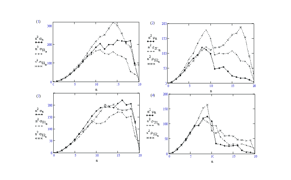
Figure 5: Quadratically scaled spectrum of singular values by standard SVD on the Logistic data $(n^{2}.\sigma_{n})$ and its surrogates $(n^{2}.\sigma_{S1_{n}})$ and $(n^{2}.\sigma_{S2_{n}})$ along with similar spectrum by nonlinear SVD for the data $(n^{2}.\rho_{n})$ and its surrogates $(n^{2}.\rho_{S1_{n}})$ and $(n^{2}.\rho_{S2_{n}})$ (i) and (ii) for the case of gaussian noise N(0,1) added noise level $27.484\%$ (iii) and (iv) and for the case of uniform noise [0,1) added noise level $28.182\%$.

As we discussed in section I, if the goal is to detect the nonlinearity but not to determine the underlying model, one could use the method suggested by A. Porta et. al. In ref porta1 the case of the logistic model itself is discussed with parameter value $\lambda=3.7$ under various noise levels. They have shown that an error function dips much further with actual data than with its surrogates. A comparison of this method and various other methods are discussed in ref  porta2 .

IX Generalization to Differential Equations

The same technique can be applied if the data is generated by a set of nonlinear differential equations. Here the goal is to identify a specific differential equation from the time series based on two assumptions (i) the sampling is frequent (ii) noise level is very low. We demonstrate here how this could be done by a combination of nonlinear SVD and the method of finding accurate derivative from data  PGV1 . Consider the following narrative. Two teams A and B are using a communication channel for sending information across each other. The sender, A is generating data from a differential equation of the form

$$\frac{d}{dt}X_{1} = X_{2}.$$ (18)

$$\frac{d}{dt}X_{2} = G(X_{1},X_{2}).$$ (19)

A time series of length 50,000 was generated using Runge - Kutta method from an initial condition $(1,-0.5)$ with sampling step size 0.001; from which a portion of $X_{1}$ of length 1000 was taken and send to team B. A hint has been given that $G$ is a relatively simple multinomial function.

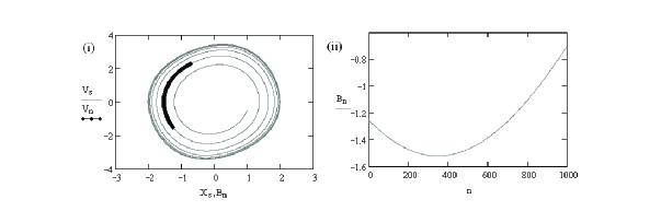
Figure 6: (i) Phase space of the original data (${X,V}$) generated by Team A ; the highlighted portion shows the section of a short data segment of length 1000; B which was sent to team B. (ii) The temporal signal B.

We illustrate the method and the issues involved by showing how team B works for the unknown differential equation with a short time series and the sampling interval. Team B is left with a small time series $Y(t)=X_{1}$ (accurate up to $10^{-16}$) shown in Fig. 5 (b) along with an information that the step size was 0.001. B calculates n derivatives of $Y(t)$ (${Y_{2},Y_{3},\ldots Y_{n+1}}$) from $Y(t)$ as mentioned in  PGV1 . $Y_{n}$ is the ${n-1}^{th}$ derivative of $Y(t)$. $Y(t)$ is denoted as ${Y_{1}}$ {the ‘$0^{th}$’ derivative of $Y(t)$} for the rest of the section. As the first step B assumes that $G$ is a nonlinear function consisting of linear and quadratic terms of $Y_{1}$ and $Y_{2}$ as shown below.

$$G=c_{1}Y_{1}+c_{2}Y_{2}+c_{3}Y_{1}^{2}+c_{4}Y_{1}.Y_{2}+c_{5}Y_{2}^{2}.$$

Hence the columns of the embedding matrix were chosen as $[{Y_{3}\ Y_{1}\ Y_{2}\ {Y_{1}}^{2}\ {Y_{2}}^{2}\ (Y_{1}Y_{2})]}$ and SVD is performed to get the singular values $(201.33,\ 162.24,\ 83.95,\ 3.95,\ 0.44,\ 0.03)$. Since the noise level is quite low, B decides to go to the next step of adding cubic terms to the embedding matrix. Now the assumed nonlinear function is,

$$G=c_{1}Y_{1}+c_{2}Y_{2}+c_{3}Y_{1}^{2}+c_{4}Y_{2}^{2}+c_{5}Y_{1}.Y_{2}+c_{6}{Y_{1}}^{3}+c_{7}{Y_{2}}^{3}+c_{8}({Y_{1}}^{2}.Y_{2})+c_{9}({Y_{2}}^{2}.Y_{1})]$$

and the corresponding embedding matrix is

$${F=[{Y_{3}\ Y_{1}\ Y_{2}\ {Y_{1}}^{2}\ {Y_{2}}^{2}\ (Y_{1}Y_{2})\ {Y_{1}}^{3}\ {Y_{2}}^{3}\ ({Y_{1}}^{2}.Y_{2})\ ({Y_{2}}^{2}.Y_{1})]}}.$$

Singular values of $F$ are (181.0635,  115.3297,  44.2941,  2.1510,  22.1215,  0.1768,  0.0247,  0.0044,  0.0003,  (2.995 $\cdot 10^{-11})$ ). Since the last singular value is very small (in the order of $10^{-11}$ ) B assumes it to be zero and tries to recover the linear relationship corresponding to that singular value. Hence the retrieved coefficient array is,

$$\hat{C}=[\ 1,\ 2.895,\ -0.237,\ 0,\ 0,\ 0,\ 0,\ 0,\ 0.237,\ 0\ ]^{T}.$$

Now team B has recovered the following equation,

$$0 = Y_{3}-0.237Y_{2}+0.237Y_{2}Y_{1}^{2}+2.895Y_{1}.$$

$$Y_{3} = 0.237Y_{2}-0.237Y_{2}Y_{1}^{2}-2.895Y_{1}.$$

$$Y_{3} = 0.237Y_{2}(1-Y_{1}^{2})-2.895Y_{1}.$$

$Y_{2}$ and $Y_{3}$ are the $1^{st}$ and $2^{nd}$ derivatives of $Y_{1}$. B has calculated 10 derivatives for this particular numerical example. When Teams A and B get together B finds that A has used Van der Pol equation of the following form with parameter values $k=2.895$ and $c=0.237$.

$$\frac{d}{dt}X_{1} = X_{2}.$$

$$\frac{d}{dt}X_{2} = cX_{2}(1-X_{1}^{2})-kX_{1}.$$

Team B’ s estimated values are $k=2.895$ and $c=0.237$ which are in agreement with the values used by A. The form of the equation and the parameter values are exactly predicted by B using the proposed method. Fig. 5 shows the phase space of Van der Pol oscillator and the temporal signal which was sent to Team B.

X Chaotic data generated by a Differential Equations

The same technique works for the chaotic data generated by a set of nonlinear differential equations. Here we explain how to identify the specific differential equation along with the parameters with the help of nonlinear SVD and the method of finding accurate derivative from data  PGV1 as explained in previous section. Consider the data generated by from the duffing equation of the form.

$$\frac{d}{dt}X_{1} = X_{2}.$$ (20)

$$\frac{d}{dt}X_{2} = -kX_{1}-cX_{2}-\delta{X_{1}}^{2}+A.cos(\omega t).$$ (21)

Let the parameter values be: $k=0.01$, $c=0.04496$, $\delta=1$, $A=1.02$ and $\omega=0.44964$. Parameters are selected such that the system exhibit chaos. We ensured adherence to the conditions (i) the sampling was frequent and (ii) noise level was very low. The time series of short length $Y(t)=X_{1}$ was sent to the receiver. The temporal signal $Y(t)$ and phase space of the duffing oscillator is displayed in Fig. 6. The receiver is informed that the data is generated using an equation of the form,

$$\frac{d}{dt}X_{1} = X_{2}.$$ (22)

$$\frac{d}{dt}X_{2} = G(X_{1},X_{2})+A.cos(\omega t).$$ (23)

Where $G$ is a low order polynomial function. Two additional information (i) sampling step size $h=0.01$ and (ii) forcing frequency $\omega=0.44964$ were given to the receiver. The parameters and the exact form of the equation can be retrieved from the data as shown below.

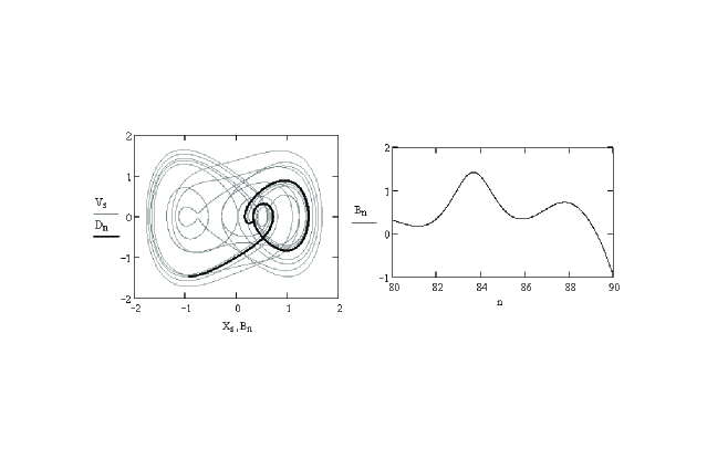
Figure 7: Phase space of the original data (${X,V}$) generated the duffing oscillator under chaos ; the highlighted portion shows the section of a short data segment of length 1000 which was used to identify the system.The temporal signal B is shown on the right side.

Once again n derivatives (${Y_{2},Y_{3},\ldots Y_{n+1}}$) are calculated. Now we assume that $G$ is a nonlinear function consisting of linear, quadratic and cubic terms of $Y_{1}$ and $Y_{2}$ along with the sinusoidal functions. $G=c_{10}Y_{1}+c_{01}Y_{2}+c_{20}Y_{1}^{2}+c_{11}Y_{1}.Y_{2}+c_{02}Y_{2}^{2}+c_{30}{Y_{1}}^{3}+c_{03}{Y_{2}}^{3}+c_{21}({Y_{1}}^{2}.Y_{2})+c_{12}({Y_{2}}^{2}.Y_{1})]+P.sin(\omega t)+Q.cos(\omega t)$. The corresponding embedding matrix is $F=[{Y_{3}\ Y_{1}\ Y_{2}\ {Y_{1}}^{2}\ {Y_{2}}^{2}\ (Y_{1}Y_{2})\ {Y_{1}}^{3}\ {Y_{2}}^{3}\ ({Y_{1}}^{2}.Y_{2})\ ({Y_{2}}^{2}.Y_{1})\sin(\omega t)\ cos(\omega t)]}$. SVD operation on $F$ gives the set of singular values (46.1294,  28.0900,  20.9784,  18.8628,  12.5940, 6.8899,  4.8714,  4.2835,  2.0742,  0.8881,  0.5682,  0). Since the last singular value is zero we can recover the linear relationship corresponding to that singular value. The coefficient array $\hat{C}$ is,

$$\hat{C}=[\ 1,\ 0.01,\ 0.04496,\ 0,\ 0,\ 0,\ 1,\ 0,\ 0,\ 0,\ -0.98958,\ 0.24723]^{T}.$$

The following equation is retrieved from $\hat{C}$.

$$Y_{3}+0.01Y_{1}+0.04496Y_{2}+1.Y_{1}^{3}-\sqrt{0.98958^{2}+0.24723}.cos(\omega t) = 0.$$

$$Y_{3}+0.01Y_{1}+0.04496Y_{2}+1.Y_{1}^{3}-1.02cos(\omega t) = 0.$$

The estimated parameter values and the form of the equation are in exact agreement with the Duffing equation from which the data was generated.

XI Linear versus nonlinear models

A second order linear system $X_{n}=a.X_{n-1}+b.X_{n-2}$ was simulated with parameter values $a=-1.5$ and $b=-1$. In the absence of noise the linear SVD had a sharper fall off than the nonlinear SVD. In the case of surrogate data neither linear SVD nor nonlinear SVD had a sharp fall off. In such cases on the grounds of parsimony alone the linear model would be chosen. In the presence of small amount of noise the same situation continues. However when the noise is beyond a certain value neither linear nor nonlinear SVD will show a substantial qualitative difference with the surrogate data to have any degree of confidence in either of the models

XII Application to Cryptanalysis

We could be interested in cryptanalysis  crptography , the study of code breaking, which involves decrypting the encrypted data, without an access to the secret key. Suppose Alice and Bob are communicating a secret across a private channel. The assumption is that the data can be read only by Bob, the intended recipient, and he has the key to decrypt the message. The aim of cryptanalysis is to decrypt the message without the key. The signal sent across the channel looks random but it is generated by a deterministic dynamical system. Since Bob has some information about the system parameters (secret key) he can retrieve the information from the encrypted signal. But the cryptanalyst, Eve is left with a random signal which is to be decrypted. All she knows about the signal is that it must have been generated by a deterministic dynamical system, preferably a non-linear one. She has no clue about the parameters or the dimension of the system. The possibility of trial and error is extremely tedious and time-consuming, and has a low probability of being successful. As compared to code-making, relatively little work has been done in cryptanalysis (hardly 1 in 100 papers propose a new method of cryptanalysis). Here we are proposing a new method based on SVD to find the information about the non-linear system from the encrypted signal. Nonlinear Singular Value Decomposition and time delayed embedding can be used to identify the nonlinearity of the system from the data. As we have discussed before, in cryptography the signals to be decoded are mostly generated by non-linear systems and complete data is not always available. A method which can extract the nonlinearity from the encrypted signal could be useful for applications in cryptanalysis. This method is potentially useful for chaotic cryptography  lakshmanan .

XIII Conclusion

We have proposed a non-linear extension of the singular value decomposition (SVD) technique by means of appending additional columns to the trajectory matrix which are non-linearly derived from the existing columns. We propose nonlinear SVD as a method which is useful for the qualitative detection and quantitative determination of nonlinearity from a short time series. We have demonstrated the utility of non-linear SVD for recovering the non-linear relationship from time series generated by discrete and continuous dynamical systems. As an example, we have demonstrated the results for the data from Logistic map, Henon Map, Van der Pol Oscillator and Duffing oscillator. The proposed method works quiet well in the presence of noise, for both Gaussian and Uniform noise (provided the noise level is not high). In principle, the method can work with any type of non-linearity. The paper contains a comparative analysis of the results for the data and its surrogates.

- (1) N. Le Bihan and J. mars, ELSEVIER Signal processing, 84, 1177 (2004); M. K. Stephen Yeung, J. Tegner, and J. J. Collins, PNAS, 99, 9, 6163 (2002); L. De Lathauwer, B. De Moor, and Joos Vandewalle, IEEE Transactions on biomedical engineering, 47, 5 (2000); O. Alter, P. O. Brown, and D. Botstein, PNAS, 18, 100, 6 (2003); Jianhua hu, F.A.Wright, and Fei Zou, Journal of the americal Statistical association, 101, 473 (2006); O. Alter, P. O. Brown, and D. Botstein, PNAS, 97, 18, 10101 (2000); B. Luo, E. R. Hancock, IEEE Transactions on Pattern Analysis and Machine Intelligence, 23, 10, 1120 (2001); Y. Takane New developments in psychometrics Yanai, H., Okada, A., Shigemasu, K., Kano, Y., and Meulman, J. (Eds.) (Springer Verlag, Tokyo, 2002).
- (2) D. S. Broomhead, G. P. King, Physica D, 217, (1986).
- (3) A. Sahay, K. R. Sreenivasan, Phil. Trans. R. Soc. Lond. A, 354, 1715 (1996).
- (4) H. D. I. Abarbanel, R. Brown, J.J. Sidorowitch, L.S. Tsimring, Rev. Mod. Phys. 65, 1331 (1993).
- (5) D. kugiumtzis, Physica D. 95, 13 (1996).
- (6) T. Buzug, G. Pfister, Physica D, 58, 127 (1992).
- (7) J. Bhattacharya, P.P. Kanjilal, Physica D 132, 100 (1999).
- (8) P. Grassberger, I. Procaccia, Physica D,9, 189 (1983).
- (9) A. R. Osborne, A. Provenzale, Physica D, 35 357 (1989).
- (10) D. Ruelle, Proc. R. Soc. Lond., 427,241 (1989).
- (11) G. Sugihara, R. May, Nature 344, 734,(1990).
- (12) B. Cazellus, B. Ferrare, Nature 25, 355 (1992) .
- (13) P. A. Ensminger, M. Vinson, J. Theor. Biol. 170, 259 (1994).
- (14) P. J. Brockwell, R. A. Davis, Introduction to time seris and forcasting, Springer-Verlag (2002).
- (15) M. J. Korenberg, Biol. Cybern., 60, 267 276, 1989.
- (16) A. Porta, G. Baselli, S. Guzzetti, M. Pagani, A. Malliani, S. Cerutti, IEEE Transactions on Biomed. Engg. 47, 12, 2000.
- (17) A. Porta, S. Guzzetti, R. Furlan, T. Gnecchi-Ruscone, N. Montano, A. Malliani, IEEE Transactions on Biomed. Engg. 54, 1, 2007.
- (18) S. Lu, K. H. Ju, Ki. H. Chon, IEEE Transactions on Biomed. Engg., 48, 10 (2001).
- (19) G. Strang, Linear Algebra and its applications (Brooks Cole, 2003).
- (20) Y. Nievergelt, SIAM Review, 36, 2, 258-264 (1994).
- (21) S. Lu, Ki H. Ju, Ki H. Chon IEEE Transactions on Signal Processing, 51, 12 (2003).
- (22) V. Z. Marmarelis, Annals of Biomed. Engg, 21, 573 (1993).
- (23) P. G. Vaidya, S. Angadi. Chaos, Solitons and Fractals, 17 ,379-386 (2003).
- (24) S. Lia, G. lvarezb, G. Chena, Chaos, Solitons and Fractals, 25, 1, 109-120 (2005) .
- (25) X. Wu , H. Hu, B. Zhang, Chaos, Solitons and Fractals Volume, 22, 2, 367-373 (2004).
- (26) P. G. Vaidya, Chaos, Solitons and Fractals 17,433 439 (2003).
- (27) W. H. Press, B. P. Flannery, S. A. Teukolsky, and W. T. Vetterling, Numerical Recipes in C: The Art of Scientific Computing (Cambridge university press, 2004).
- (28) R. C. Gonzales and R. E. Woods, Digital Image Processing (Addison-Wesley Publishing Company, 1992).
- (29) Takens, Lecture Notes in Mathematics, 898 (1981).
- (30) J. Theiler, S. Eubank, A. Longtin, B. Galdrikian, J.D. Farmer, Physica D 58 (1992) 77; M.B. Kennel, S. Isabelle, Phys. Rev. A 46 (1992) 3111.
- (31) A. Menezes, P. C. Van Oorschot, and S. Vanstone , Handbook of Applied Cryptography (CRC Press Florida, 1996).
- (32) M. Lakshmanan and S. Rajaseekar, Nonlinear Dynamics: Integrability Chaos and Patterns (Springer, 2002).