Detecting very-high-frequency relic gravitational waves by electromagnetic wave polarizations in a waveguide

Abstract

The polarization vector (PV) of an electromagnetic wave (EW) will experience a rotation in a region of spacetime perturbed by gravitational waves (GWs). Based on this idea, Cruise’s group has built an annular waveguide to detect GWs. We give detailed calculations of the rotations of the polarization vector of an EW caused by incident GWs from various directions and in various polarization states, and then analyze the accumulative effects on the polarization vector when the EW passes $n$ cycles along the annular waveguide. We reexamine the feasibility and limitation of this method to detect GWs of high frequency around $100$ MHz, in particular, the relic gravitational waves (RGWs). By comparing the spectrum of RGWs in the accelerating universe with the detector sensitivity of the current waveguide, it is found that the amplitude of the RGWs is too low to be detected by the waveguide detectors currently running. Possible ways of improvements on detection are discussed also.

1 Introduction

GW is one of important predictions of general relativity. Although there has been an indirect evidence of GW radiation from the binary pulsar B1913+16 [1], so far direct detection of GWs have not been accomplished yet. GWs can have different frequencies generated by various kinds of sources. Currently, besides the conventional method of cryogenic resonant bar [2], a number of detectors using new techniques have been running or under construction aiming at direct signals of GWs. For a frequency range $1\sim 10^{4}$ Hz, the method of ground-based laser interferometers applies, such as LIGO [3], Virgo [4], and TAMA [5], . For a lower frequency range $10^{-4}\sim 1$ Hz, the space-based laser interferometers can be used, such as LISA [6] under planning. For much lower frequencies $\sim 10^{-18}$ Hz, detections of CMB polarization of “magnetic” type would also give direct evidence of GWs [7]. There have also been attempts to detect GWs of very high frequencies from MHz to GHz, employing various techniques, such as laser beam [8]. One interesting method proposed by Cruise uses linearly polarized EWs [9, 10]. When GWs pass through the region of waveguide, the direction of PV of EWs will generally experience a rotation [9]. A prototype gravitational waves detector has been built by Cruise’s group [10], which consists mainly of one, or several, annular waveguide of a shape of torus. As a merit of this method, depending upon the size of the waveguide, GWs in a very high frequency range $10^{6}\sim 10^{9}$ Hz can be detected, which is not covered by the laser interferometer method. Note that the GWs in the frequency range $10^{6}\sim 10^{9}$ Hz are generally not generated by usual astrophysical processes, such as binary neutron stars, binary black holes, merging of neutron stars or black holes, and collapse of stars [11] [12]. However, the background of RGWs has a spectrum stretching over a whole range of $10^{-18}\sim 10^{11}$ Hz [13, 14]. Depending on the frequency ranges, its different portions can be detected by different method. For instance, the very low frequency range $10^{-18}\sim 10^{-16}$ Hz can be detected by the curl type of polarization in CMB [7], the low frequency range $10^{-3}\sim 10^{-2}$ Hz can be detected by LISA, the mediate frequency range $10^{2}\sim 10^{3}$ Hz is covered by LIGO, and the very high frequency range $10^{6}\sim 10^{9}$ Hz can be the detection object of Cruise’s EWs polarization method. Therefore, one of the main object of detection by the annular waveguide is the very high frequency RGWs. The detection of high frequency RGWs from MHz to GHz is in complimentary to the usual detectors working in the range of $10^{-4}\sim 10^{4}$ Hz. RGWs is a stochastic background that are generated by the inflationary expansion of the early Universe [13, 14, 15, 16, 17], and its spectrum depends sensitively on the inflationary and the subsequent reheating stages. Besides, the currently accelerating expansion also affects both the shape and the amplitude of the RGW spectrum [13, 14, 17]. RGWs carry take a valuable information about the Universe, therefore, their detection is much desired and will provide a new window of astronomy.

In this paper we give a comprehensive study of the rotations of PV of EWs in a conducting torus caused by incident GWs, and explore the feasibility and limitation of Cruise’s method of detecting GWs by polarized EWs in the annular waveguide. Firstly, we briefly review the RGWs in the currently accelerating universe. Secondly, we shall present detailed calculations of rotations of the PV of EWs in the waveguide caused by the incoming GWs from from various directions and in various polarization states, thereby we analyze the multiple-cycling accumulating effect and the resonance when the circling frequency of EWs is nearly equal to that of GWs. Thirdly, we shall examine the possible detection of the RGWs by the annular waveguide system around 100 MHz, comparing the predicted spectrum of RGWs in the accelerating Universe with the sensitivity of the detector [10]. Finally, we give the conclusions and possible ways of improvements for detection.

2 Relic gravitational waves

In an expanding universe RGWs can be regarded as small perturbations to the Robertson-Walker metric,

$${\mathrm{d}}s^{2}=a^{2}(\tau)[\,-{\mathrm{d}}\tau^{2}+(\delta_{ij}+h_{ij})\,{\mathrm{d}}x^{i}{\mathrm{d}}x^{j}],$$ (1)

where $a(\tau)$ is the scale factor, $\tau$ is the conformal time, and $h_{ij}$ is transverse-traceless

$$\partial_{i}\,h^{ij}=0,\qquad\ \delta^{ij}\,h_{ij}=0,$$ (2)

representing RGWs. Among six components $h_{ij}$ there are only two independent (two polarization states). Generally, $|h_{ij}|\ll 1$. The wave equation for RGWs is

$$\partial_{\mu}\,(\sqrt{-g}\,\partial^{\mu}\,h_{ij}({\mathbf{x}},\tau))=0.$$ (3)

The solution $h_{ij}$ of Eq.(3) and the spectrum $h(\nu,\tau_{H})$ defined via

$$<h^{ij}h_{ij}>=\int_{0}^{\infty}h^{2}(k,\tau_{H})\frac{{\mathrm{d}}k}{k}$$ (4)

have been given for an accelerating universe [14, 17, 18]. Fig.1 plots $h(\nu,\tau_{H})$, which depends on the accelerating parameter $\gamma$, the inflation parameter $\beta$, the reheating parameter $\beta_{s}$, the tensor/scalar ratio $r$, and the redshift $z_{E}$ at the time $\tau_{E}$ of equality of dark energy and matter is given by

$$1+z_{E}=\frac{a(\tau_{H})}{a(\tau_{E})}\simeq(\frac{\Omega_{\Lambda}}{\Omega_{m}})^{\frac{1}{3}}.$$ (5)

Since the annular waveguide is to detect RGWs of frequencies $\sim 10^{8}$ Hz, we quote the analytic approximate spectrum in this range [14]:

$$h(k,\tau_{H})\approx A_{0}(\frac{k_{s}}{k_{H}})^{\beta_{s}}\frac{k_{H}}{k_{2}}(\frac{k}{k_{H}})^{\beta-\beta_{s}+1}\frac{1}{(1+z_{E})^{3+\epsilon}},$$ (6)

where $k$ is the comoving wavenumber related to the physical frequency by $\nu=\frac{k}{2\pi a(\tau_{H})}$, $A_{0}$ is a constant determined by the CMB anisotropies [7, 14, 18, 19], $\epsilon\equiv(1+\beta)(1-\gamma)/\gamma$ is a small parameter, and $k_{H}=2\pi\gamma$ and $k_{s}\simeq 10^{26}k_{H}$. Note that the RGWs $h_{ij}$ described above exist everywhere and all the time in the Universe. We may simply say that the Universe is filled with a stochastic background, consisting of all the modes of different wave-vector $k^{\mu}$=$(k^{0},k^{1},k^{2},k^{3})$. So the RGWs serve as an object for GWs detections.

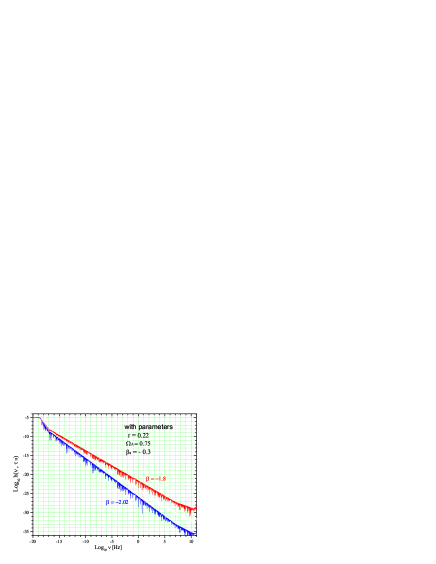
Figure 1: The spectrum $h(\nu,\eta_{H})$ of RGW in the accelerating universe.

In the frequency range $\sim 100$ MHz for the waveguide detector, RGWs can be approximated as plane waves. A beam of monochromatic plane GWs with a wave-vector can be generally written as the following form [20]

$$h_{ij}=Re\{A_{ij}e^{i\phi}\},$$ (7)

where $A_{ij}$ represents the amplitude and $\phi$ is the phase of GWs,

$$\phi=k_{\mu}x^{\mu}=g_{\mu\nu}k^{\mu}x^{\nu},$$ (8)

with $x^{\mu}$ being the point of spacetime that the waves pass.

3 The Annular Waveguide

Consider an annular waveguide of shape of a torus, as shown Fig.2. Its radius is $R$, and the cross section is a rectangle with sides $a>b$, both being much less than $R$, say, $a,b\sim 1$ cm, and $R\sim 1$ m. (Note that the waveguide actually employed by Cruise’s group [10] actually has a shape of rectangle, instead of a torus. For simplicity of analysis, here we consider a torus since the working mechanism is the same.) Inside the torus, one can input a beam of linearly polarized EW propagating around the toroidal loop, and the beam consists of a ${\mathrm{TE}_{10}}$ mode (transverse electric field) with the electric field $\bf E$ pointing along the $x^{3}-$axis. The EWs are a microwave, say, with a wavelength $\lambda_{e}\sim 1$ mm and a frequency $\nu_{e}=c/\lambda_{e}\sim 10^{11}$ Hz. The guided EWs of ${\mathrm{TE}_{10}}$ mode in the torus travel around the loop at a group speed [21],

$$v=c\sqrt{1-(\frac{\lambda_{e}}{2a})^{2}},$$ (9)

where $c$ is the speed of light, and $v$ is very close to $c$. For instance, for $\lambda_{e}\sim 1$mm and $a=1$cm, the difference between the two velocities is $\sim(\lambda_{e}/2a)^{2}/2\sim 10^{-3}$. As is well-known, for a TE₁₀ mode to exist in the waveguide, one has to $\lambda_{e}\leq 2a$. The angular velocity of EWs cycling around the loop is then

$$\omega_{0}=\frac{v}{R}\simeq\frac{c}{R}.$$ (10)

As will be seen later, when the angular frequency $\omega$ of the incident GWs is very close to the $\omega_{0}$, i.e., at the resonant condition, the detector responds most sensitively to the GWs. Therefore, such a device of given radius $R$ will primarily detect GWs of a resonant frequency around

$$\nu_{g}\simeq\frac{c}{2\pi R}.$$ (11)

For example, if the radius is $R=1$ m, then the frequency of GWs to be detected is $\nu_{g}\simeq 5\times 10^{7}$ Hz, some two orders smaller than $\nu_{e}$. As a merit, by adjusting the size $R$, the frequency of GWs to be detected can vary accordingly. For the 4-dim spacetime, one can choose a coordinate system $\{x^{\mu}\}$ with $\mu=0,1,2,3$ and $x^{0}\equiv ct$, such that the waveguide lies on the $(x^{1},x^{2})$ plane as shown in Fig.2. Note that the geometric size $R$ of waveguide is negligibly small in comparison with the Hubble’s radius $\sim c/H$, so that the effect of cosmic expansion on the torus can be totally neglected.

Let us consider a beam of GWs passing through the detector. Assume that the wavelength $\lambda_{g}$ of the GWs is much longer than the wavelength $\lambda_{e}$ of the EWs in the waveguide, i.e., $\lambda_{g}\gg\lambda_{e}$, so that the geometric optics approximation applies in describing the EWs [9, 20]. In fact, this assumption on the incident GWs is automatically satisfied if the GWs satisfy the resonant condition. The PV of the linearly polarized EWs can be described by a 4-vector, $\Pi^{\mu}=(\Pi^{0},\Pi^{1},\Pi^{2},\Pi^{3})$, which is real and normal to the wave vector $P^{\mu}$ of the EWs

$$\Pi_{\mu}P^{\mu}=0,$$ (12)

and satisfies the normalized condition [20, 9]

$$\Pi_{\mu}\Pi^{\mu}=1.$$ (13)

Eq.(12) tells that one can add a multiple of $P^{\mu}$ to $\Pi^{\mu}$ without affecting any physical measurements [20], since $P^{\mu}$ is a null vector with $P_{\mu}P^{\mu}=0$. Suppose that the EWs are propagating along the $x^{1}-$axis with the wave vector $P^{\mu}=(P^{0},P^{1},0,0)$, which satisfies $P_{\mu}P^{\mu}=0$. Then, by Eq.(12), the PV of EWs can be generally written as $\Pi^{\mu}=(\kappa P^{0},\kappa P^{1},\Pi^{2},\Pi^{3})$, where $\kappa$ is an arbitrary constant. Then, Eq.(13) leads to

$$|\Pi^{2}|^{2}+|\Pi^{3}|^{2}=1.$$ (14)

Since initially the electric field $\mathbf{E}$ of the EWs inside the torus is set to be along the $x^{3}-$ axis and $\Pi^{i}$ is, by definition, in the direction of $\mathbf{E}$, so the initial PV is

$$\Pi^{\mu}=(\,0,0,0,1),$$ (15)

i.e., initially the PV has a vanishing $\Pi^{2}=0$ component.

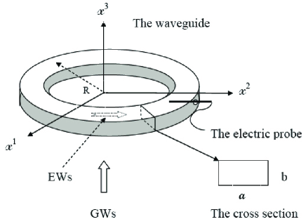
Figure 2: A sketch map of the annular waveguide. The cross section of the waveguide is rectangle with $a$ and $b$ being much less than the radius $R$. EWs travel inside the waveguide and GWs propagate along the $x^{3}$-axis.

However, the presence of GWs will cause a rotation of the $\Pi^{\mu}$ about the direction of propagation, generating a non-vanishing $\Pi^{2}\neq 0$ i.e., a component $E^{2}\neq 0$ of the electric field $\mathbf{E}$ of the EWs in the waveguide. One puts an electric field probe inside the waveguide at the intersection of the $x^{2}-$ axis and the torus. The probe is on the line of $x^{2}$ axis, so that it can probe the non-vanishing electric field $E^{2}$ due to the rotation of $\bf E$ caused by the GWs [10]. The GWs induce an electric voltage on the electric probe $V=E_{0}\alpha\,l\,\sin{(2\pi\nu_{e}t)}$, where $E_{0}$ is the ${\mathrm{TE}}_{10}$ mode electric field in the waveguide, $l$ is the length of the conducting probe.

In the geometric optics approximation, the motion of $\Pi^{\mu}$ is described as being parallel-propagating along the rays of Ews with the equation

$$\frac{d\Pi^{\mu}}{ds}+\Gamma_{\nu\sigma}^{\mu}\Pi^{\nu}\frac{dx^{\sigma}}{ds}=0,$$ (16)

where $s$ is an affine parameter, which can be chosen to be $s=t/T_{0}$ with $T_{0}=2\pi/\omega_{0}$ being the period of the EWs travelling around the torus. Note that when $s$ goes from $0$ to $1$, the EWs go one cycle around the torus. Since $a,b\ll R$, one can view the EWs in the waveguide as travelling along the $1-$dimensional loop path

$$x^{\mu}=R\left(\frac{2\pi cs}{v},-\sin{2\pi s},\cos{2\pi s},0\right),$$ (17)

where $v$ is the group speed of the EWs.

With the initial setup of the polarization of EWs in the torus, we only need to consider the component $\Pi^{2}$ of the polarization in the following.

4 Change of $\Pi^{2}$

Even the setup of the waveguide detector is fixed in laboratory, GWs propagating in space may come in any direction randomly. Therefore, we need to determine the rotation of polarization of EWs caused by GWs travelling along the directions $x^{i}$, $i=1,2,3$, respectively.

A. GWs travelling along the positive $x^{3}$-axis

Consider a beam of monochromatic plane GWs travelling along the positive $x^{3}$-axis with a wave vector $k^{\mu}=(2\pi/\lambda_{g},0,0,2\pi/\lambda_{g})$. As the GWs just pass the annular waveguide whose position is given by Eq.(17), then substituting it into Eq.(8) yields the phase of the GWs at the point inside the annular waveguide

$$\phi=-2\pi s\,\omega/\omega_{0}.$$ (18)

Here $\omega=2\pi c/\lambda_{g}$ represents the angular frequency of GWs, and $\omega_{0}=(2\pi/T_{0})$ is the cycling angular frequency of EWs around the torus. As mentioned before, one can take the flat spacetime slightly perturbed by GWs to represent the local region of the waveguide. In the transverse traceless (TT) gauge, the metric tensor can be written as

$$g_{\mu\nu}=\eta_{\mu\nu}+h_{\mu\nu}=\left(\begin{array}[]{cccc}-1&0&0&0\\ 0&1+h_{\oplus}&h_{\otimes}&0\\ 0&h_{\otimes}&1-h_{\oplus}&0\\ 0&0&0&1\end{array}\right),$$

and

$$g^{\mu\nu}=\eta^{\mu\nu}-h^{\mu\nu}=\left(\begin{array}[]{cccc}-1&0&0&0\\ 0&1-h_{\oplus}&-h_{\otimes}&0\\ 0&-h_{\otimes}&1+h_{\oplus}&0\\ 0&0&0&1\end{array}\right),$$

where $h_{\oplus}$ and $h_{\otimes}$ denote the $+$ and $\times$ modes of polarization of GWs, respectively. In general, these two modes of GWs may be not coherent, i.e. their phases are random and independent, a situation similar to the natural light of EWs. If the $+$ and $\times$ modes have the same phase $\phi$, which is called as the linearly polarized GWs [20], then by Eq.(7) one has

$$h_{\oplus}=A_{\oplus}\cos{\phi},\,\,\,\,h_{\otimes}=A_{\otimes}\cos{\phi},$$ (19)

where $A_{\oplus}$ and $A_{\otimes}$ are real numbers. This case of a linearly polarized GWs will be discussed in the following, otherwise we give a clear indication.

As can be checked, the change in $\Pi^{3}$ due to GWs is of order of $|h_{ij}|^{2}$, so in the subsequent calculation, $\Pi^{3}=1$ is assumed. To calculate the change of $\Pi^{2}$ up to the linear order of $h_{ij}$, one needs the following Christoffel components

$$\Gamma_{31}^{2}=-\pi A_{\otimes}\sin{\phi}/\lambda_{g},$$

$$\Gamma_{32}^{2}=\pi A_{\oplus}\sin{\phi}/\lambda_{g},$$ (20)

other components are either zero or of order $|h_{ij}|^{2}$, having no contributions. Integrating Eq.(16) gives the expression of the change in $\Pi^{2}$ around one circle of the torus

$$\Delta\Pi^{2}=\int_{0}^{1}\frac{d\Pi^{2}}{ds}ds=-\int_{0}^{1}\left(\Gamma_{31}^{2}\Pi^{3}\frac{dx^{1}}{ds}+\Gamma_{32}^{2}\Pi^{3}\frac{dx^{2}}{ds}\right)ds.$$ (21)

Substituting Eqs.(17) and (4) into the integration, one has

$$\Delta\Pi^{2}=\frac{2\pi^{2}R}{\lambda_{g}}\int_{0}^{1}\left(A_{\otimes}\sin{\bigg{(}2\pi s\frac{\omega}{\omega_{0}}\bigg{)}}\cos{2\pi s}-A_{\oplus}\sin{\bigg{(}2\pi s\frac{\omega}{\omega_{0}}\bigg{)}}\sin{2\pi s}\right)ds.$$ (22)

Carrying out integration yields the result

$$\Delta\Pi^{2}=\frac{A_{\otimes}}{2}\left(1-\cos{(2\pi\varpi)}\right)\frac{\varpi^{2}}{\varpi^{2}-1}-\frac{A_{\oplus}}{2}\sin{(2\pi\varpi)}\frac{\varpi}{\varpi^{2}-1},$$ (23)

where $\varpi\equiv\omega/\omega_{0}$. So the change of $\Pi^{2}$ depends on $\omega$.

Let us see what a value $\Delta\Pi^{2}$ will take when the cycling angular frequency of EWs is equal to the angular frequency of GWs,

$$\omega_{0}=\omega,$$ (24)

called the resonant condition. Taking the limit $\varpi\rightarrow 1$ in Eq.(23) yields a constant value

$$\Delta\Pi^{2}=-\frac{\pi A_{\oplus}}{2},$$ (25)

which has only contribution from the $+$ mode. This is the known result by Cruise [9].

Let us discuss other special cases of Eq.(23).

(1) If the GWs are given such that $A_{\oplus}=0$, i.e., there is only the $\times$ mode,

$$\Delta\Pi^{2}=\frac{A_{\otimes}}{2}\left(1-\cos{(2\pi\varpi)}\right)\frac{\varpi^{2}}{\varpi^{2}-1},$$ (26)

which is plotted in Fig. 3 as a function of $\varpi$. It shows that $\Delta\Pi^{2}$ can be both positive and negative, depending on $\varpi$. A maximum value of $\Delta\Pi^{2}$ is achieved at $\varpi\simeq 1.434$.

Figure 3: The $\Delta\Pi^{2}$ as an oscillating function of $\varpi$ when $A_{\oplus}=0$. $\Delta\Pi^{2}$ has a maximal value of $1.864A_{\otimes}$ at $\varpi=1.434$ and a minimal value of $-0.643A_{\otimes}$ at $\varpi=0.743$. Also notice that: (1) $\Delta\Pi^{2}=A_{\otimes}$, for $\varpi\gg 1$ and $\varpi$ equals half integer; (2) $\Delta\Pi^{2}=0$, for $\varpi$ equals integer; (3) $\Delta\Pi^{2}=0$, for $\varpi\rightarrow 0$.

(2) If the GWs are given such that $A_{\otimes}=0$, i.e., there is only the $+$ mode,

$$\Delta\Pi^{2}=-\frac{A_{\oplus}}{2}\sin{(2\pi\varpi)}\frac{\varpi}{\varpi^{2}-1},$$ (27)

which is shown in Fig. 4. A minimum value of $\Delta\Pi^{2}$ is achieved at $\varpi\simeq 1.036$.

Figure 4: The $\Delta\Pi^{2}$ as a function of $\varpi$ when $A_{\otimes}=0$. $\Delta\Pi^{2}$ has a minimum $-1.585A_{\oplus}$ at $\varpi=1.036$.

Figure 5: The $\Delta\Pi^{2}$ as a function of $\varpi$ when $A_{\otimes}=A_{\oplus}=A$. $\Delta\Pi^{2}$ has a maximum $1.842$ at $\varpi=1.546$ and a minimum $-1.802$ at $\varpi=0.889$.

(3) If $A_{\otimes}=A_{\oplus}=A$, where $A$ is real, as is likely the case for relic gravitational waves, then one gets

$$\Delta\Pi^{2}=\frac{A}{2}(\varpi-\varpi\cos(2\pi\varpi)-\sin(2\pi\varpi))\frac{\varpi}{\varpi^{2}-1},$$ (28)

which is shown in Fig.5 that is the compound of Fig. 3 and Fig. 4.

Instead of a linearly polarized GWs in Eq.(19), consider the case of circularly polarized GWs with $A_{\oplus}=iA_{\otimes}=A$,

$$h_{\oplus}=A\cos{\phi},\,\,\,\,\,h_{\otimes}=A\sin{\phi}.$$ (29)

By similar calculations, one has the relevant Christoffel components

$$\Gamma_{31}^{2}=\pi A\cos{\phi}/\lambda_{g},$$

$$\Gamma_{32}^{2}=\pi A\sin{\phi}/\lambda_{g},$$ (30)

Integrating Eq.(21) yields

$$\Delta\Pi^{2}=\frac{A\varpi\sin{(2\pi\varpi)}}{2(1+\varpi)},$$ (31)

which is shown in Fig.6.

Figure 6: The relation between $\Delta\Pi^{2}$ and $\varpi$ for circularly polarized GWs. The value of $\Delta\Pi^{2}$ will always less than $A/2$.

B. GWs travelling along the positive $x^{1}$-axis

Different from the above, consider a plane GWs travelling along the positive $x^{1}$-axis. The wave vector is $k^{\mu}=2\pi/\lambda_{g}(1,1,0,0)$. Then, by Eqs.(8) and (17), the phase of GW in the torus is

$$\phi=-2\pi x^{0}/\lambda_{g}+2\pi x^{1}/\lambda_{g}=-(2\pi s+\sin{(2\pi s)})\omega/\omega_{0}.$$ (32)

The metric is now

$$g_{\mu\nu}=\eta_{\mu\nu}+h_{\mu\nu}=\left(\begin{array}[]{cccc}-1&0&0&0\\ 0&1&0&0\\ 0&0&1+h_{\oplus}&h_{\otimes}\\ 0&0&h_{\otimes}&1-h_{\oplus}\end{array}\right).$$

Similar calculations give the relevant Christoffel components

$$\Gamma_{30}^{2}=\pi A_{\otimes}\sin{\phi}/\lambda_{g},$$

$$\Gamma_{31}^{2}=-\pi A_{\otimes}\sin{\phi}/\lambda_{g},$$ (33)

and the change in $\Pi^{2}$ around one circuit of the path

$$\Delta\Pi^{2}=\frac{2\pi^{2}rA_{\otimes}}{\lambda_{g}}\int_{0}^{1}(1+\cos{(2\pi s)})\sin{\bigg{(}\frac{\omega}{\omega_{0}}(2\pi s+\sin{(2\pi s)})\bigg{)}}ds.$$ (34)

Integrating Eq.(34) gives rise to

$$\Delta\Pi^{2}=A_{\otimes}\sin^{2}{(\pi\varpi)}$$ (35)

which is oscillates between $A_{\otimes}$ and $0$. Note that the $A_{\oplus}$ has no contribution.

In the case of circularly polarized GWs, Eqs.(4) and (34) should be replaced by

$$\Gamma_{30}^{2}=-\pi A\cos{\phi}/\lambda_{g},$$

$$\Gamma_{31}^{2}=\pi A\cos{\phi}/\lambda_{g},$$ (36)

and

$$\Delta\Pi^{2}=\frac{2\pi^{2}rA}{\lambda_{g}}\int_{0}^{1}(1+\cos{(2\pi s)})\cos{\bigg{(}\frac{\omega}{\omega_{0}}(2\pi s+\sin{(2\pi s)})\bigg{)}}ds,$$ (37)

and one has

$$\Delta\Pi^{2}=\frac{A}{2}\sin{(2\pi\varpi)},$$ (38)

oscillating between $A/2$ and $-A/2$.

c. GWs travelling along the positive $x^{2}$-axis

When the plan GWs travel along the positive $x^{2}$-axis, the metric tensor of spacetime is

$$g_{\mu\nu}=\eta_{\mu\nu}+h_{\mu\nu}=\left(\begin{array}[]{cccc}-1&0&0&0\\ 0&1+h_{\oplus}&0&h_{\otimes}\\ 0&0&1&0\\ 0&h_{\otimes}&0&1-h_{\oplus}\end{array}\right).$$

Similar calculations show that the relevant Christoffel components are $0$, and thus

$$\Delta\Pi^{2}=0.$$ (39)

Thus, the GWs travelling along $x^{2}$-axis will not change $\Pi^{2}$. Therefore, to avoid a null result of detection in case of an incident GWs in the $x^{2}$ direction, one may put two probes with $90^{0}$ separation along the annular waveguide.

5 Accumulative effect

When the EWs pass $n$ cycles along the annular waveguide, the change of $\Pi^{2}$ may be accumulative. This is of practical significance in actual detections. We need only consider GWs along the $x^{3}-$ and the $x^{1}-$ directions.

Firstly, for the linearly polarized incident GWs in the $x^{3}-$ direction, integrating Eq.(22) form $0$ to $n$ gives the change of $\Pi^{2}$ for $n$ cycles

$$(\Delta\Pi^{2})_{n}=\frac{A_{\otimes}}{2}\left(1-\cos{(2\pi n\varpi)}\right)\frac{\varpi^{2}}{\varpi^{2}-1}-\frac{A_{\oplus}}{2}\sin{(2\pi n\varpi)}\frac{\varpi}{\varpi^{2}-1}.$$ (40)

In the special case $A_{\otimes}=0$, Fig.7 gives a plot of $(\Delta\Pi^{2})_{n}$ for $n=10$. In contrast with Fig.6 for $n=1$, $(\Delta\Pi^{2})_{n}$ is now sharply peaked at $\varpi\simeq 1$ with a much larger amplitude, as a prominent feature. As given in Table 1, under the resonance condition $\varpi\rightarrow 1$, the amplitude of $(\Delta\Pi^{2})_{n}$ increases linearly with $n$. In fact, this linearly-increasing amplitude $\Delta\Pi^{2}_{\mathrm{min}}$ at very large $n$ is also obtained by taking the resonance limit $\varpi\rightarrow 1$ of Eq.(40), yielding

$$(\Delta\Pi^{2})_{n}=-\frac{n\pi A_{\oplus}}{2},$$ (41)

which is in accord with the result obtained by Cruise [9].

Table 1: The case $A_{\otimes}=0$. The amplitude of $(\Delta\Pi^{2})_{n}$ increases linearly with $n$, as $\varpi\rightarrow 1$.

n	$\varpi_{\rm{min}}$	$\Delta\Pi^{2}_{\rm{min}}/A_{\oplus}$
$1$	$1.036$	$-1.585$
$10$	$1.00038$	$-15.71$
$100$	$\sim 1$	$-157.08$
$1000$	$\sim 1$	$-1570.8$
$2000$	$\sim 1$	$-3141.6$
$10000$	$\sim 1$	$-15708$

Figure 7: The case of $A_{\otimes}=0$ and $n=10$. $(\Delta\Pi^{2})_{n}$ has a minimal $-15.071A_{\oplus}$ at $\varpi=1.00038$.

The special cases of $A_{\oplus}=0$ and of $A_{\oplus}=A_{\otimes}$ are quite similar to each other. $(\Delta\Pi^{2})_{n}$ has, for each given $n$, both a sharp maximum $\Delta\Pi^{2}_{max}$ at $\varpi_{max}>1$ and a sharp minimum $\Delta\Pi^{2}_{min}$ at $\varpi_{min}<1$. As $n\rightarrow\infty$, the amplitudes $\Delta\Pi^{2}_{max}$ and $\Delta\Pi^{2}_{min}$ increase with $n$ approximately linearly, and their locations $\varpi_{max}$ and $\varpi_{min}$ approach to $1$ from either side, respectively. Fig.8 and Fig.9 give the plots of $(\Delta\Pi^{2})_{n}$ with $n=10$ for $A_{\oplus}=0$ and for $A_{\oplus}=A_{\otimes}$, respectively. Table 2 and Table 3 list the increase with $n$ of the amplitudes of extrema $\Delta\Pi^{2}_{max}$ and $\Delta\Pi^{2}_{min}$ for $A_{\oplus}=0$ and for $A_{\oplus}=A_{\otimes}$, respectively.

Table 2: The case $A_{\oplus}=0$. The amplitudes of extrema of $(\Delta\Pi^{2})_{n}$ increase with $n$.

n	$\varpi_{\rm{max}}$	$\Delta\Pi^{2}_{\rm{max}}/A_{\otimes}$	$\varpi_{\rm{min}}$	$\Delta\Pi^{2}_{\rm{min}}/A_{\otimes}$
1	1.434	1.864	0.743	-0.643
10	1.038	12.027	0.964	-10.761
100	1.0037	114.456	0.9963	-113.189
1000	1.00037	1138.85	0.99963	-1137.58
2000	1.00019	2277.07	0.99982	-2275.8
10000	1.00004	11382.8	0.999963	-11381.5

Table 3: The case $A_{\oplus}=A_{\otimes}$. The amplitudes of extrema of $(\Delta\Pi^{2})_{n}$ increase with $n$.

n	$\varpi_{\rm{max}}$	$\Delta\Pi^{2}_{\rm{max}}/A_{\otimes}$	$\varpi_{\rm{min}}$	$\Delta\Pi^{2}_{\rm{min}}/A_{\otimes}$
1	1.546	1.842	0.889	-1.802
10	1.055	11.05	0.982	-20.214
100	1.0055	103.504	0.9981	-205.148
1000	1.00055	1028.1	0.99981	-2054.59
2000	1.00027	2055.43	0.999907	-4109.52
10000	1.00005	10274.1	0.999981	-20549

Figure 8: The case of $A_{\oplus}=0$ and $n=10$. $(\Delta\Pi^{2})_{n}$ has a maximum $\Delta\Pi^{2}_{max}=12.027A_{\otimes}$ at $\varpi=1.038$, and a minimal $\Delta\Pi^{2}_{min}=-10.761A_{\otimes}$ at $\varpi=0.964$.

Figure 9: The case of $A_{\otimes}=A_{\oplus}=A$ and $n=10$. $(\Delta\Pi^{2})_{n}$ has a maximum $\Delta\Pi^{2}_{max}=11.05A$ at $\varpi=1.055$, and a minimal $\Delta\Pi^{2}_{min}=-20.214A$ at $\varpi=0.982$.

For circularly polarized GWs in the $x^{3}-$ direction, the $n-$ cycle result is

$$(\Delta\Pi^{2})_{n}=\frac{A\varpi\sin(2\pi n\varpi)}{2(1+\varpi)},$$ (42)

which does not accumulate with $n$, but vibrates more rapidly than Eq.(31).

Secondly, for the lineal polarized incident GWs in the $x^{1}-$ direction, the $n-$ cycle result is

$$(\Delta\Pi^{2})_{n}=A_{\otimes}\sin^{2}{(n\pi\varpi)},$$ (43)

which has no accumulating effect. For the circularly polarized GWs in the $x^{1}-$ direction

$$(\Delta\Pi^{2})_{n}=\frac{A\sin(2n\pi\varpi)}{2},$$ (44)

having no accumulating effect, either.

So the above detailed analysis on the $n$-cycle accumulating effects yields the simple conclusion: Only linearly polarized incident GWs in the $x^{3}$-axis has a linearly accumulating effect of rotation of PV of EWs in the limit $\varpi\rightarrow 1$. Theoretically, in order to experimentally obtain a maximum effect of $n$-cycle accumulation, the circling EWs in the waveguide should be running so that $n$ is as large as possible. Of course, due to attenuation of EWs in the actual waveguide, for a given waveguide made of conducting metal, such as copper, an input beam of EWs in the waveguide can run only a finite number of turns around the torus. The maximum value of $n$ is approximately equal to the quality factor $Q$, mainly determined by the conducting metal employed and the pump resonances. For instance, Cruise’s group [10] has used copper for the waveguide, and the measured value of the quality factor $Q\simeq 2000$. As for the selective response of the detector to the particular $x^{3}-$ direction of the incident GWs under the resonant condition $\omega\simeq\omega_{0}$, it is a problem for gravitational radiations from certain sources, since they generally exist for a finite short period of time (from minutes to hours) and have some fixed direction of propagation. But for the RGWs as the detection object, it is not a problem at all, as they consist of various modes in all directions and of all frequencies, moreover, they are a stochastic background existing everywhere and all the time. Therefore, the RGWs serve as a natural object of detection. What one needs to do is to set up a convenient position of the torus and to fix the the cycling angular frequency $\omega_{0}=v/R$ of EWs around the waveguide. There are always modes of the RGWs with the $x^{3}$ direction and the angular frequency $\omega\simeq\omega_{0}$.

6 Detecting capability for very high frequency RGW

Let us examine the capability of the waveguide detector built up by Cruise’s group [10], particularly in regards to the RGWs. Consider the favorable case of GWs travelling along the $x^{3}-$direction. Since the rotation $\Delta\Pi^{2}$ is small, it is equal to the angle $\alpha$ rotated, $\alpha\simeq\Delta\Pi^{2}$. This angle can be measured by the electric probe. In general, the detector sensitivity will be limited by the thermal noise in the electronic amplifiers. It has been found that [10] the minimum detectable angle of rotation

$$\alpha_{\rm{min}}=\sqrt{\frac{ab\,kTB}{fPl^{2}}},$$ (45)

where $f$ is an efficiency factor of the probe, which transfers electric signals to the following electronic amplifiers, $k$ is the Boltzmann’s constant, $T$ is the amplifier noise temperature, and $B$ is the detector bandwidth in hertz. Thus, for a constant amplitude on the time scale $\sim Q/\nu_{0}$, during which the EWs travel $Q$ turns around the loop, by Eq.(41), the minimum detectable amplitude $h_{min}$ of the GWs is

$$h_{min}=\frac{2}{\pi}\frac{\alpha_{min}}{Q}=\frac{2}{\pi}\sqrt{\frac{abkTB}{fP_{\rm{in}}Q^{3}l^{2}}},$$ (46)

where the input power $P_{in}$ is related to the circulating power $P$ by $P_{in}=P/Q$. Here $Q$ is the quality factor of the waveguide. For a random signals of GWs with amplitude varying considerably over the time scale $\sim Q/\nu_{0}$, the minimum detectable amplitude is

$$h_{\rm{min}}=\frac{2}{\pi}\sqrt{\frac{abkTB}{fP_{\rm{in}}Q^{2}l^{2}}},$$ (47)

since the angle $\alpha$ of rotation accumulatively increases as $\alpha\propto\sqrt{Q}$ as for a random walk.

The waveguide detector is used to monitor the GWs of frequency $\sim 10^{8}$ Hz, which primarily come from the stochastic background of RGWs with a very broad frequency range ($10^{-18}\sim 10^{10}$) Hz [14, 17, 18]. The RGW spectrum $h(\nu,\eta_{H})$ as given by Eq.(6) in a frequency range $>10^{7}Hz$ depends sensitively on the reheating parameter $\beta_{s}$. The spectra for three different values of $\beta_{s}=0.5,\,0,\,-0.3$, respectively, are given in Fig.10 for a model with $\beta=-1.8$, $r=0.22$, and $\Omega_{A}=0.75$. A larger $\beta_{s}$ has a lower amplitude in the range $(10^{7}\sim 10^{9})$ Hz, however, around $\nu\geq 10^{9}$ Hz the spectrum begins to increase considerably. Therefore, if the detector is capable of accurately detecting the RGWs signals, it will, in principle, be able to constrain the model parameters $\beta$ and $\beta_{s}$, and distinguish different models of reheating during the early universe.

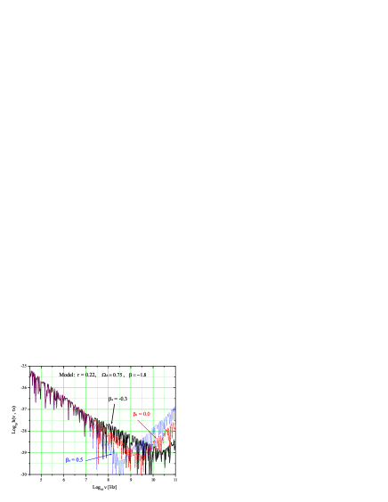
Figure 10: The spectrum $h(\nu,\eta_{H})$ with different parameter $\beta_{s}$ for $\beta=-1.8$.

Other sources of GWs, such as binary neutron stars or black holes, merging of neutron stars or black holes can produce GWs, but the frequency is much lower than $10^{8}$ Hz [12]. Thus they are not to be detected by the waveguide detector discussed here. There might be other astrophysical processes, which can give rise to high frequency GWs [22]. Thermal gravitational radiation of stars can generate GWs at most probable frequencies $\sim 10^{15}$ Hz. But this frequency is too high for the waveguide detector [22] [23]. The predicted graser beams in interstellar plasma can generate GWs with “optical” frequencies $>10^{12}$ Hz, still too high for the waveguide detector [24]. The GW radiation from primordial black holes of small mass $M\leq 10^{-5}M_{\odot}$ can generate GWs with frequencies $\geq 10^{10}$ Hz, which is too high for the waveguide detector. Besides the rate of event is very low $\sim 5\times 10^{-2}$events/year/galaxy [25]. Therefore, our primary object of detection is RGWs, whose spectrum in the current accelerating universe is derived in Refs.[14, 17].

What the waveguide detector actually detects is the root-mean-square (r.m.s.) amplitude of RGWs per Hz^1/2 at a given $\nu$, which can be written simply as [18]

$$\frac{h(\nu)}{\sqrt{\nu}},$$ (48)

where $h(\nu)$ denotes the value of the spectrum $h(\nu,\eta_{H})$ given in Eq.(6). Since the waveguide detector works around the frequency $10^{8}$ Hz, so we need to examine the value of $h(\nu,\eta_{H})$ around this frequency predicted by our calculation [14, 17]. For a cosmological model with the tensor/scalar ratio $r=0.22$, the dark energy $\Omega_{\Lambda}=0.75$, and the reheating $\beta_{s}=0.3$, one directly reads from Fig.1 the values $h(\nu)\simeq 10^{-28},10^{-34}$ for the values of the inflationary parameter $\beta=-1.8$, $-2.02$, respectively. So the corresponding r.m.s amplitude per $Hz^{1/2}$ at $\nu=10^{8}Hz$ is then

$$\frac{h(\nu)}{\sqrt{\nu}}\simeq(10^{-32},\,\,\,\,10^{-37})\,\,Hz^{-1/2},$$ (49)

for the two values of $\beta$, respectively. On the other hand, the detector sensitivity can be improved by using the cross correlation of two or multiple detectors. From a short run of some $4$ seconds of the two detectors, Ref.[10] gives the cross correlation sensitivity,

$$5\times 10^{-15}Hz^{-1/2},$$ (50)

which is within a factor $4$ of the predicted sensitivity given that parameters $P_{in}=69mW$, $T=300$K, $Q=2000$, $(ad)/l^{2}=0.5$, and $f>0.9$. By comparing the preliminary experimental result in Eq.(50) with the predicted values in Eq.(49), it is clear that the predicted value of RGWs in the model $\beta=-1.8$ is lower than the prototype detector sensitivity by $17$ orders. As has been analyzed in Ref.[10], the detector sensitivity of the current detector could be improved by a factor of $10^{4}\sim 10^{5}$, through optimization of the transducers, use of cryogenic amplifiers and multiple detector correlation. But even with these possible improvements, still that will be some $12$ orders short to able to measure the predicted amplitude of RGWs in Eq.(49).

An interesting feature of the spectrum of RGWs is that it has a higher amplitude in lower frequencies. This may be suggestive for new ways of enhancing the chance of detections. As is seen from Eq.(11), if one increases the radius $R$ of the annular waveguide, say to from $1$ meter to $100$ meters, the frequency of GWs to be detected will subsequently be reduced to a low value $\nu_{g}\simeq 5\times 10^{5}$ Hz, at which the spectral amplitude $h(\nu,\eta_{H})$ increases by a factor $\sim 10^{3}$, as is seen from Fig.1. The r.m.s amplitude per Hz^1/2 will be $h(\nu)/\sqrt{\nu}\sim 10^{-28}$ Hz^-1/2. Now, this is only some $8$ orders lower than the detector sensitivity of the improved device. Therefore, according to our calculation of RGWs, it is unlikely to detect signals of RGWs, using the annular waveguide detectors as it stands today. But enlarging the radius $R$ will enhance the detection probability considerably, of course, at the price of a larger sum of cost and a more complex construction. By the way, note that LIGO is still unable to detect the RGWs by 2 orders of magnitude even it has achieved its design sensitivity [17]. Moreover, theoretically, there are possibilities that the waveguide detector can detect signals from other kinds of sources of GWS with a much improved sensitivity.

7 Conclusions

From the calculations of the rotation of PV of EWs, it is found that the detector only essentially responds to the linearly polarized RGWs travelling in the $x^{3}$-axis under the resonant condition. Both the circularly polarized RGWs travelling along any direction and the linearly polarized RGWs travelling in the $x^{1}$- or $x^{2}$-axis have not observable effect. But these propose no problem for the RGWs as the object of detection.

From our analysis comparing the spectrum of GRWs with the detector sensitivity, the RGWs in the accelerating universe have a very low amplitude and are not possible to detect using this current detector. The gap between them is some 17 orders of magnitude under the current experiment conditions. Even with the improvements on the current detector system as planned in [10], there will still be a gap of $12$ orders of magnitude. Examining the detector itself, Eq.(46) and Eq.(47) tell that the sensitivity of the detector can be directly improved by several means as follows: (1) The use of cryogenic devices at lower temperature $T$ of the environment, i.e., to reduce thermal noise of the amplifiers; (2) Increasing the quality factor $Q$ of the waveguide, so that the EWs can travel more number of turns around the loop path; (3) Enhancing the input power $P_{in}$ of the EWs into the waveguide; (4) Using multiple detectors, whose correlation can improve the sensitivity of the detector. On the other hand, the shape of the RGWs spectrum $h(\nu)$ is such that its amplitude is higher in lower frequencies. Therefore, it may be more promising to detect the RGWs in the relative lower frequency range. For instance, if the radius of torus is increased to $R=100$ meter, the detecting frequency $\nu_{g}\sim 5\times 10^{5}$ Hz, and the gap will reduced down to $8$ orders of magnitude. An overall estimate is that significant improvements of the current prototype detector are needed for a possible detection of RGWs by the waveguide.

ACKNOLEDGMENT: We thank Dr. A.M. Cruise for helpful suggestions. Y.Zhang’s work was supported by the CNSF No.10173008, SRFDP, and CAS.

References

- [1] Hulse R. A., Taylor J. H., 1975, ApJ, 195, L51; Weisberg J. M., Taylor J. H., 2004, in Binary Radio Pulsars, ASP Conference Series, Vol. TBD.
- [2] Allen Z. et al, 2000 Phys. Rev. Lett, 85, 5046; Aston P. et al, 2001 Class. Quant. Grav, 18, 243
- [3] Abramovici A. et al, 1992, Science 256, 325
- [4] Bradaschia C. et al, 1990, Nucl.Instrum.Methods Phys.Res.A, 289, 518
- [5] Takahashi H., Tagoshi H., the TAMA Collaboration, 2004 Class. Quant. Grav, 21, S697-S702
- [6] Jafry Y., Corneliss J., Reinhard R., 1994, ESA Bull, 18, 219
- [7] Seljak U., Zaldarriaga M., 1997, Phys. Rev. Lett, 78, 2054; Kaminkowski M., Kosowski A,, Stebbins A., 1997, Phys. Rev. D, 55, 7368; Pritchard L. P., Kaminkowski M., 2005 Ann. Phys.(N.Y.), 318, 2; Zhao W., Zhang Y., 2006, Phys. Rev.D, 74, 083006; Baskaran D., Grishchuk L. P., Polnarev A. G., 2006, Phys. Rev. D74 () 083008
- [8] Li F.-Y. et al, 2003, Phys. Rev. D 67, 104008 Li F.-Y. et al, 2006, Int. J. Mod. Phys, gr-gc/0604109 Li F.-Y., Tang M.-X., Luo J., Li C.-Y., 2000, Phys. Rev. D, 62, 044018
- [9] Cruise A. M., 1983, MNRAS, 204, 485; Cruise A. M., 2000, Class. Quantum. Grav, 17, 2525
- [10] Cruise A. M., Ingley R. M. J., 2005, Class. Quantum. Grav, 22, s479 Cruise A. M., Ingley R. M. J., 2006, Class. Quantum. Grav, 23, 6185
- [11] Grishchuk L. P., et al, 2001, Phys. Usp., 44, 1
- [12] Zhang Y., Zhao W., Yuan Y. F., 2004, Publications of Purple Moutain Observary, 23, 53
- [13] Grishchuk L. P., 1975, Sov.Phys. JETP, 40, 409 Grishchuk L. P., 1997, Class. Quant. Grav., 14, 1445
- [14] Zhang Y. et al, 2005, Class. Quant. Grav., 22, 1383 Zhang Y. et al, 2005, Chin. Phys. Lett., 22, 1817 Zhang Y. et al, 2006, Class. Quant. Grav., 23, 3783
- [15] Giovamini M, 1999 Class.Quant.Grav. 16 2905; 1999 Phys.Rev.D60 123511
- [16] Zhao W., Zhang Y., 2006, Phys. Rev. D, 74, 043503
- [17] Miao H. X., Zhang Y., 2007, Phys. Rev. D, 75, 104009
- [18] Grishchuk L. P. 2001 in Lecture Notes in Physics, 562, 167 (Preprint gr-qc/0002035)
- [19] Spergel D. N. et al, 2003, ApJ Suppl., 148, 175
- [20] Misner C. W., Thorne K. S., Wheeler J. A., 1973, Gravitiation (San Francisco, Freeman) pp570-580, pp952-954
- [21] Li C.-Z., Zhao F.-Z., 1997, Electrodynamics Tutorial (Publishing Company of National University of Defense Technology)
- [22] Bisnovatyi-Kogan G. S., Rudenko V. N., 2004, Class. Quantum. Grav., 21, 3347
- [23] Weinberg S., 1972, Gravitation and Cosmology; Galtsov D. V., Gratz Yu., 1974, Sov. Phys.–JETP, 17, 94
- [24] Servin M., Brodin G, 2003, Phys. Rev. D, 68, 044017
- [25] Nakamura T. et al, 1997, ApJ, 487, L139