Habitable Climates

Abstract

According to the standard liquid-water definition, the Earth is only partially habitable. We reconsider planetary habitability in the framework of energy-balance models, the simplest seasonal models in physical climatology, to assess the spatial and temporal habitability of Earth-like planets. We quantify the degree of climatic habitability of our models with several metrics of fractional habitability. Previous evaluations of habitable zones may have omitted important climatic conditions by focusing on close Solar System analogies. For example, we find that model pseudo–Earths with different rotation rates or different land–ocean fractions have fractional habitabilities that differ significantly from that of the Earth itself. Furthermore, the stability of a planet’s climate against albedo-feedback snowball events strongly impacts its habitability. Therefore, issues of climate dynamics may be central in assessing the habitability of discovered terrestrial exoplanets, especially if astronomical forcing conditions are different from the moderate Solar System cases.

1 Introduction

Planetary science is being challenged by extrasolar planetary system discoveries (Mayor & Queloz, 1995; Marcy & Butler, 1996). The orbital architectures of many of these systems, with massive planets located either very near to their parent stars or on highly eccentric orbits, are strikingly unusual. These discoveries have been surprising, however, mostly as a consequence of our own Solar-System centric point of view. In fact, planet searches at multi-AU orbital distances are now providing tentative evidence that Solar System giant planets, with their nearly circular orbits, are more the exception than the norm, by simple comparison with the ensemble properties of known extrasolar planetary systems (Marcy et al., 2005). If these preliminary trends hold, they may have a profound impact on our perception of our place in the Universe.

The pace of exoplanet discoveries has accelerated sharply in the last few years and the future looks bright. Two significant developments in exoplanet research have occurred within the last year or so. A micro-lensing discovery of a likely terrestrial planet, with a mass $5.5$ times that of Earth, was reported by Beaulieu et al. (2006), making it the first discovery of a planet that is thought to be terrestrial (i.e. rocky). Several months ago, Udry et al. (2007) announced the Doppler-velocimetry discovery of a potentially habitable terrestrial planet around a low-mass M-dwarf. In considering future discoveries, of specific interest to this study are two dedicated space missions: Corot and Kepler (Baglin, 2003; Borucki et al., 2003, 2007). A key objective of both missions is to monitor a large number of stars to detect the (repeatable) micro-eclipses generated when terrestrial planets transit in front of their host star. It is expected that a few Earth analogues (i.e. with Earth-like masses and comparable distances to their host stars), and possibly hundreds to thousands of additional terrestrial planets unlike Earth, will be identified by Corot and Kepler after a few years of operation (Borucki et al., 2007, 2003; Basri et al., 2005). The discovery of an Earth-like exoplanet, potentially hosting life as we know it, is therefore within the 5-year astronomical horizon. Ambitious missions are also being prepared to map in detail the orbits of exoplanets around nearby stars (with SIM PlanetQuest (Unwin et al., 2007)) and later to obtain spectra of nearby Earth-like planets in the hope that they would reveal the first unambiguous signatures of life on a remote world (with the Terrestrial Planet Finder and Darwin (Leger & Herbst, 2007)).

The idea that liquid surface water is a prerequisite for a terrestrial planet to have the ability to host life is widely used as the key concept behind searches for habitable planets around other stars. This is because of the central and critical role that water plays in the biochemistry on Earth. As the current exoplanet census indicates, notions based on an old Solar System centric view may only be relevant to a minority of planets (or planetary systems). What if most terrestrial planets discovered in the future have, like the vast majority of exoplanets currently known, highly eccentric orbits generating large seasonal variations? What if the atmospheric mass and composition, planetary spin rate, or land-sea coverage of these exo-Earths are generally different from what they are on Earth? If the last ten years of extrasolar planet discoveries offer any guidance, our Solar System appears to show but little of the general planetary diversity found around other stars.

The classical calculations of habitability on Earth-like planets by, e.g., Dole (1964) and Hart (1979) predated extrasolar discoveries. Apart from a few exceptions (Franck et al. 2000; Gaidos et al. 2005; see also von Bloh et al. 2007; Selsis et al. 2007 in the specific context of the Gleise 581 system) the subject of planetary atmospheric habitability has been revisited little since the seminal work of Kasting et al. (1993). Given the major developments expected in the next five years and beyond, it is important that the climate regimes expected on exotic versions of the Earth, and their consequences for habitability, be studied and better understood. This will help interpret upcoming planet detections and will inform future long-term efforts on the best strategies to find robust signatures of life on exo-Earths.

The central role of astronomical forcings in determining the seasons and the climatology of the Earth is well known (e.g., the long-term Milankovitch cycles). Clearly, obliquity, precession, and eccentricity can all strongly affect global and regional habitability conditions on the Earth and, by extension, on any other potentially habitable terrestrial exoplanet. Previously, only preliminary investigations of the role of obliquity (Williams & Kasting 1997, hereafter WK97; and Williams & Pollard 2003) and eccentricity (Williams & Pollard, 2002), for very specific Earth-like conditions, have been considered in some detail. The surface habitability of a terrestrial planet, however, must depend on the combination of obliquity and eccentricity with the planetary rotation rate, the continental coverage (from dry Earths to water worlds) and the overall mass and composition of the atmospheric layer (e.g., compare Mars vs. Venus), among other factors. A thorough exploration of how these various global planetary attributes combine to affect climatology and make a terrestrial planet seasonally or regionally habitable is therefore an important element in the search for signatures of life elsewhere. In the present study, we describe how energy balance climate models can contribute to this understanding.

In § 2, we introduce the concept of climate modeling hierarchy, describe our energy balance model and validate it on the Earth. In § 3, we reconsider various features of habitability for Earth–like planets with seasonally-forced climates. In § 4, we discuss several subtleties in the definition of habitability that emerge from our work on seasonal climates, and we finally conclude in § 5.

2 Climate Modeling Hierarchy

Current modeling tools to study the Earth’s climate are constructed to be specific to Earth. For example, their radiative transfer schemes are elaborate and specific to the conditions of Earth’s atmosphere and are valid only within fairly narrow ranges of atmospheric composition, temperature and pressure. Their surface boundary conditions are also specific to a given land-ocean-ice configuration. The same is essentially true of advanced climate tools used to model the atmospheres of Mars or Venus. This strongly limits the region of planetary parameter space that can be explored with these computationally intensive tools. Such models are bound to produce a somewhat limited view of what constitutes a habitable planet. They have been useful in providing some initial insights on astronomical factors affecting habitability (e.g., Williams & Pollard 2002, 2003), but given the likely detection of terrestrial exoplanets with various global attributes in the near future, it is important that tools addressing the specific needs of astronomers be developed now, to help assess the potential habitability of discovered exoplanets.

A difficult aspect of assessing the habitability of discovered terrestrial exoplanets will be that many of the key planetary attributes that determine the climate regime will remain entirely unknown to astronomers, at least in the foreseeable future. Consider, for instance, the terrestrial planets that will be discovered by Kepler. While their semimajor axes, their radii, and thus indirectly their masses and surface gravities (e.g., Valencia et al. 2006, 2007; Fortney et al. 2007; Adams et al. 2007) may be reasonably well constrained by the data – but see Seager et al. (2007) – very little additional information on the global planetary attributes will be available to help us evaluate their potential habitability. In some special cases, it may be possible to set constraints on orbital eccentricities (Barnes, 2007; Ford et al., 2008), but in general, except for tidally-locked planets, the eccentricity, obliquity and planetary rotation rate will all be essentially unknown. Perhaps even more important, the atmospheric mass and composition of detected planets will be unknown. Even though an incremental amount of information on rocky exoplanets will become gradually available with future generations of space missions (i.e., orbits with SIM-PlanetQuest and later spectra with TPF and Darwin), this bright future does not alleviate the need for an interpretation of Kepler, COROT, and radial velocity exoplanet discoveries in terms of habitability.

To address this interpretational challenge, one approach is to consider the climate problem at a fundamental level, using first principles to systematically classify planets whose climate regimes and associated surface physical conditions might permit habitability. As we shall see below, an approach based on 1-dimensional Energy Balance Models (EBMs) is particularly attractive because it is computationally efficient. This approach, therefore, permits a relatively thorough exploration of the multi–dimensional parameter space of planetary properties in order to identify the most promising regions of that space for habitability.

In physical climatology (e.g., Hartmann 1994; Ghil 2002), a hierarchical family of climate models has been built from tools of increasing complexity. At the lowest level of the hierarchy, quantitative descriptions of planetary climate start with simple, global radiative balance models. These models focus on a steady radiative equilibrium solution, associate a single surface temperature to an entire planet, and ignore important equator-to-pole dynamical atmospheric fluxes. They cannot account for the time–variable property, nor the regional property of climate and habitability. It is significant that, even though much of Earth itself is only transiently or regionally habitable by the standard liquid water criterion, calculations of habitability for astronomical applications have almost exclusively relied on global radiative balance models, of the type described in Kasting et al. (1993). As a result, existing work on habitability has largely emphasized radiative and chemical issues. Tackling the equally important dynamical ones requires regional and seasonal climate models.

At the next level of the hierarchy, 1-dimensional EBMs solve a 1D time-dependent diffusion equation to specify the evolution of the surface temperature as a function of planetary latitude, based on seasonal variations in incoming and outgoing radiative fluxes and the energetic redistribution due to atmospheric motions. In the presence of a thick enough atmosphere, dynamical transport is indeed an important contributor to the local thermal budget of a terrestrial planet and therefore affects its regional habitability properties. Ever since the seminal work of Budyko (1969) and Sellers (1969) on the Earth’s climate, 1D EBMs have been recognized as useful tools in physical climatology, especially for studies of variations in external (astronomical) forcing conditions and their effects on climate stability (Hartmann, 1994). Except for a few preliminary investigations (e.g., WK97; Franck et al. (2000); Gaidos & Williams (2004)), however, 1D EBMs have generally not been applied to the outstanding problem of habitability on terrestrial exoplanets.

In the present work, we describe EBMs for planets that are largely similar to Earth, partly because this permits us to validate our new modeling tool on this well known and understood case. In the course of presenting our models, we will use two terms, “Earth–like” and “pseudo–Earth”, to distinguish between model planets that are, within the context of our 1-dimensional energy balance framework, as similar to Earth as we can achieve with very simple heating and cooling functions (“Earth–like”) and model planets that are less specifically tuned to Earth by virtue of, e.g., having a different rotation rate (“pseudo–Earth”). We investigate how the habitability of our pseudo–Earths varies with their distance from a sun–like star, and with the efficiency of the latitudinal redistribution of heat. In this study, we consider only cases with 0 orbital eccentricity and an Earth-like 23.5-degree obliquity. As illustrated below, we already find that the issue of habitability for close Earth analogs becomes a rich one when addressed with a 1D time-dependent EBM.

2.1 Global Radiative Balance

It is instructive to start our investigation of habitable climates with a discussion of global radiative balance results. Assuming that the annual mean surface temperature, $T$, on an Earth–like planet is determined by radiative balance between energy sources and sinks, the following steady-state radiative equilibrium equation must be satisfied,

$$I[T]=S(1-A[T]),$$ (1)

where $I$ is the infrared cooling flux, $S$ is the annual mean stellar insolation flux and $A$ is the global planetary albedo.

In this work, we consider three different formulations for the cooling and albedo functions. Compared to previous work on global radiative balance (e.g. Kasting et al., 1993), our treatment is extremely simple. Nevertheless, it accounts for the key physical elements involved in the absorption and reemission of incident stellar flux and is sufficient for our EBM work, which is focused on dynamical climate issues rather than radiative transfer ones.

In a planetary atmosphere, the greenhouse effect acts to reduce the infrared cooling flux, $I[T]$, at a given value of the surface temperature, $T$. Kasting (1988) and Kasting et al. (1993), for instance, describe in detail how the Earth’s greenhouse effect scales with surface temperature. An important result is that higher temperatures cause greater humidity, which in turn leads to stronger atmospheric heat retention via the greenhouse effect from water vapor absorption (see also WK97). Our purpose here is not to accurately reproduce Earth’s climate but rather to investigate dynamic climate issues for Earth-like planets. We therefore consider three different models for the infrared cooling function, $I$, and the albedo function, $A$, as listed in Table 1. While each of these models reproduces reasonably well the current climate of the Earth, (see § 2.2.2), they could each respond differently once we start exploring physical conditions that are different from the current Earth. These three atmosphere models are therefore useful in evaluating the sensitivity of our main results on habitable climates to detailed model assumptions for the infrared cooling and albedo functions.

Models 1 and 2 have infrared cooling functions inspired from a one-zone radiative transfer formulation that assumes ground-level blackbody emission ($\sigma T^{4}$), effectively reduced at the atmospheric “photosphere” according to a near-Eddington approximation (inspired by Shu (1982)), for a given atmospheric optical thickness to infrared radiation, $\tau_{\rm IR}$ (as shown in Table 1). Model 3, on the other hand, adopts the standard linear cooling function of North & Coakley (1979), which can be interpreted as a linearization of IR–cooling around the globally-averaged conditions for the Earth. It is in close agreement with other T-linearized IR models used in the geophysical literature (e.g., Budyko, 1969; North et al., 1981). In our model 1, the IR optical thickness is fixed to unity, while in model 2, a cubic dependence on surface temperature, $T$, is adopted, to better match the linear model results (model 3) for Earth-equivalent conditions.

In each of our three atmospheric models, the albedo function, $A[T]$, is chosen to capture a rapid ice-water transition, with values of $A\sim$ 0.7–0.77 well below 263 K (ice–covered surface), and values $\sim$ 0.25–0.3 well above 273 K (ice–free surface). To avoid albedo discontinuities, which are known to result in spurious “small ice-cap” instabilities in EBMs (e.g., Held et al. (1981)), the albedo transition is performed smoothly over the range 263–273 K with a hyperbolic tangent formulation. This type of albedo prescription is standard in the context of EBMs (e.g. WK97). The slightly different asymptotic values adopted for the albedos in our three models (see Table 1) were adjusted to best reproduce the annual mean climate of the Earth. This is common practice with simplified EBMs which do not account for the detailed land-surface conditions that contribute to the global planetary albedo (see § 2.2.1 for a discussion of EBM limitations).

In what follows, we adopt model 2 as our fiducial model but we also show a few comparison results with models 1 and 3. Quite generally, we find that predictions from our three atmospheric models differ only modestly at a quantitative level. With a choice of IR-cooling and albedo functions, steady-state radiative equilibrium solutions for the annual mean climate are obtained by solving Eq. (1) for a specified value of the annual mean insolation flux, $S$, received by the planet. For a fast-spinning planet, such that a diurnal average is justified, on a circular orbit at a distance $a$ (in AU) from a Sun-like star, the annual mean insolation is simply $S=(1/4)\,S_{0}/a^{2}$ (e.g. Rubincam 2004), where the solar constant $S_{0}=1.36\times 10^{6}$ erg cm^-2 s^-1.

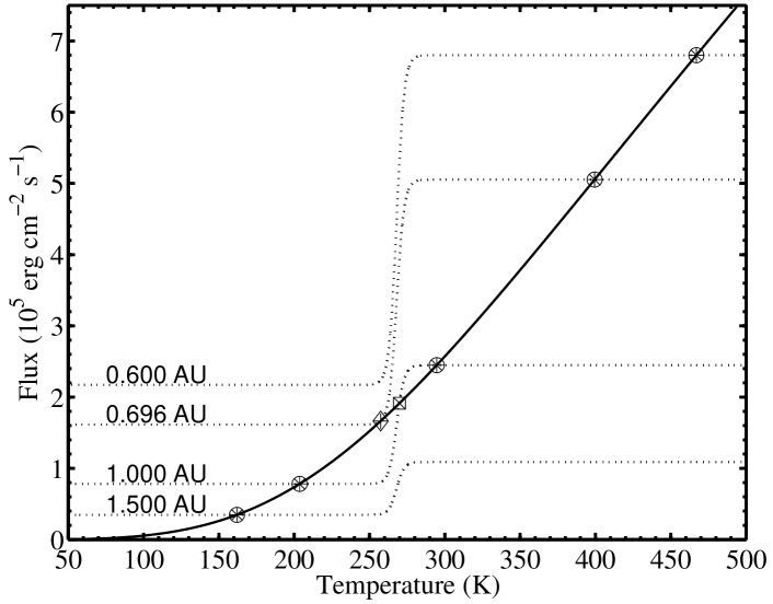
Figure 1: Heating and cooling fluxes, as a function of surface temperature, in a global radiative balance model using the IR-cooling and albedo functions listed as model 2 in Table 1. The solid line shows the IR-cooling flux while dotted lines show albedo-reduced, annual mean insolation fluxes at four different orbital distances from a Sun–like star (from 0.6 AU to 1.5 AU). Stable radiative equilibrium solutions are highlighted with circles. Other solutions are thermally unstable (see text for details). In the vicinity of $\sim 1$ AU, this class of global radiative balance models generally admits two stable solutions for the climate; one is ice-free and the other is ice-covered.

With these assumptions, Eq. (1) reduces to the thermal balance equation $Q^{-}=Q^{+}$, where the annual mean cooling rate, $Q^{-}=I[T]$, and heating rate, $Q^{+}=(1-A[T])S$, are expressed per unit surface area of the planet. Due to the steep albedo variation with surface temperature, relative to the smooth IR-cooling dependence, it is possible for multiple climate equilibrium solutions to satisfy Eq. (1). Figure 1 illustrates this possibility, using our model 2 for definiteness. The cooling and heating rates, $Q^{-}$ and $Q^{+}$, are shown as solid and dotted lines, respectively, for a wide range of surface temperatures. The heating rate is shown at four different orbital distances from the central Sun-like star, from $0.6$ to $1.5$ AU. The strong effect of the albedo transition on the heating rate is easily identified at $T\simeq 263$–$273$ K.

While unique climate equilibrium solutions satisfy Eq. (1) for $a=0.6$ and $1.5$ AU, two such solutions are found at $a=0.696$ AU and three solutions are found at $a=1$ AU, as shown by the intersections of dotted and solid lines in Fig. 1. Solutions to a thermal balance equation such as Eq. (1) are stable only if small increases in temperature cause cooling to exceed heating and small decreases cause heating to exceed cooling:

$$\frac{d\left(Q^{+}-Q^{-}\right)}{dT}<0,$$ (2)

If the above equation is satisfied, then any small surface temperature perturbation relaxes back to the starting equilibrium solution. Figure 1, then, shows that solutions found in the steep part of the albedo transition ($T\simeq 263$–$273$ K) are generally unstable, given the relatively slow increase of the IR-cooling flux with surface temperature. The intermediate temperature solution in the case $a=1$ AU is therefore unstable and the lower temperature solution in the marginal case $a=0.696$ AU is stable only on one side (stable against reductions in temperature but not against increases).

At small or large enough orbital distances, a unique stable solution exists, corresponding to either an ice-free or an ice-covered climate. At intermediate orbital distances ($\sim 1$ AU), however, both the ice-free and the ice-covered climate solutions are valid and stable. This bi-stable property of Earth’s climate in simple global radiative balance models is well-known and it may be related to the snowball (globally ice-covered) events for which there is some evidence in the past history of Earth’s climate (see the review by Hoffman & Schrag (2002) and references therein). We also note that these ice-covered equilibrium solutions correspond to the “cold-start” scenarios briefly mentioned by Kasting et al. (1993) in their detailed study of habitability with global radiative balance models.

Globally ice-covered climate solutions are often omitted from studies of planetary habitability because they violate the standard surface liquid water requirement for habitability. Yet, Earth’s climate itself may have experienced one or two such global glaciation events and recovered from them without catastrophic damage to life on the planet, or at least without eradicating life from the planet (Hoffman et al., 1998; Hoffman & Schrag, 2000; Baum & Crowley, 2003; Hoffman & Schrag, 2002). The fact that the current Earth is partially ice–covered, depending on the seasons, reveals another obvious shortcoming of global radiative balance calculations for habitability: an Earth-like planet can be habitable even if it is regionally and/or transiently ice-covered. This important class of climate regime is simply not addressed by global radiative balance models admitting only fully ice-covered or fully ice-free stable solutions, as illustrated in Fig. 1. The present work on seasonally habitable climates is motivated precisely by the possibility to explore these more complex climate regimes with a simple class of climate models.

2.2 1–D Energy Balance Model

Issues of seasonal climate dynamics and susceptibility to climate transitions are not addressed by steady–state radiative balance models that consider only annually averaged global mean conditions. In principle, one can solve for the instantaneous radiative equilibrium conditions either locally or globally on an Earth–like planet. A planet satisfying radiative equilibrium globally, however, does not necessarily satisfy it locally, for two main reasons: First, atmospheric motions tend to transport heat from the hotter regions to the colder regions, effectively coupling the thermal states of various locations on the planet beyond a simple state of radiative balance. Second, the atmosphere has thermal inertia and does not immediately adjust its temperature to the local forcing. As a result, local radiative equilibrium solutions will generally not be accurate representations of local surface temperature conditions. Furthermore, because of this thermal inertia, planets do not necessarily satisfy even global radiative equilibrium, especially when on eccentric orbits. These important physical processes can be incorporated in a time–dependent EBM that models the seasonal climate as a latitudinal diffusion of atmospheric heat under prescribed astronomical forcing.

A justification of the equivalent diffusion equation satisfied by an atmospheric layer, obtained by averaging the second law of thermodynamics and the continuity equation, can be found in Lorenz (1979). Lorenz (1979) also argues that the diffusion approximation is justified for the Earth, on large enough scales for the atmosphere to be considered a forced system. Following WK97 and previous work in the geophysical literature, we adopt the following prognostic diffusion equation for the planetary surface temperature,

$$C\frac{\partial T[x,t]}{\partial t}-\frac{\partial}{\partial x}\left(D(1-x^{2})\frac{\partial T[x,t]}{\partial x}\right)+I[T]=S(1-A[T]),$$ (3)

where all quantities are local functions, $x\equiv\sin\lambda$ is the sine of the latitude $\lambda$, $T$ is the surface temperature, $C$ is the effective heat capacity of the atmosphere (different over land, ocean, and ice), $D$ is the diffusion coefficient that determines the efficiency of latitudinal redistribution of heat, $I$ is the same IR-cooling flux as in §2.1, $S$ is the diurnally-averaged insolation flux and $A$ is the same albedo function as in §2.1. In the above equation, $C$, $D$, $I$, and $A$ are functions of $T$, $x$, $t$, and possibly other relevant planetary parameters. The $(1-x^{2})$ factor multiplying the diffusion coefficient in Eq. (3) is a standard prescription to capture the reduced efficiency of latitudinal heat transport in the polar regions of an Earth-like planet (see, e.g., North et al. (1983)).

Our prescriptions for $C$ and $D$ are borrowed from WK97 and the existing geophysical literature on 1D EBMs. For simplicity and flexibility, we use simple, physically motivated prescriptions. For the surface heat capacity $C$, we assume a uniform ocean fraction of $70\%$ at every latitude and use the same partial heat capacities over land, ocean, and ice as WK97: $C_{l}=5.25\times 10^{9}\,{\rm erg~{}cm^{-2}~{}K^{-1}}$ over land, $C_{o}=40\,C_{l}$ above the wind-mixed surface layer of the ocean, $C_{i}=9.2\,C_{l}$ over ice when $263<T<273{\rm~{}K}$, and $C_{i}=2.0\,C_{l}$ for $T\leq 263{\rm~{}K}$ (see WK97 for details). For the diffusion coefficient $D$, we adopt a fiducial value that is adjusted to reproduce the current climate of Earth and is $93\%$ of that used by WK97: $D_{\rm fid}=5.394\times 10^{2}{\rm~{}erg~{}cm^{-2}~{}s^{-1}~{}K^{-1}}$. For the diurnally-averaged insolation flux $S$, we use the same standard formalism as WK97 (see their Appendix). Throughout this work, we adopt an Earth-like planetary obliquity, $i=23.5$°, and assume zero eccentricity of the planetary orbit for simplicity.

Equation (3) is solved on a grid uniformly spaced in latitude with a highly efficient time-implicit numerical scheme and an adaptive time–step, as described in Hameury et al. (1998). We impose the boundary conditions $dT/d\lambda=0$ at $\lambda=\pm 90\arcdeg$ for symmetrical solutions. Resolution tests, which are further described in Appendix I, show excellent numerical convergence at our fiducial resolution corresponding to $1.25\arcdeg$ in latitude (145 grid points pole–to–pole). All models are initiated with a uniform temperature corresponding to an ice-free planet. To guarantee satisfactory relaxation to a periodically-forced, seasonal climate regime that is unaffected by details in initial conditions, all models are integrated for at least 130 years, well in excess of the thermal-inertial timescale of about a decade of the modeled atmospheric layer. As shown in Appendix II, specific choices of initial conditions can potentially influence long-term model outcomes by inducing a dynamical transition to a fully ice-covered (snowball) climate even when ice-free initial conditions are specified. We systematically initialize our models with temperatures well above freezing (e.g., $T\;\hbox to0.0pt{\lower 2.5pt\hbox{$\sim$}\hss}\raise 1.5pt\hbox{$>$}\;300$ K for Earth-like planets), which guarantees that partially ice-covered climates are favored over fully ice-covered snowball states. This is similar to excluding “cold start” scenarios in global radiative balance studies of habitability (e.g., Kasting et al. 1993).

To summarize, we make the following assumptions in the models presented here:

1. Heating/Cooling – The heating and cooling functions are given by the diurnally averaged insolation from a sun–like (1 $M_{\sun}$, 1 $L_{\sun}$) star, with albedo and insolation functions given in Table 1.

2. Latitudinal Heat Transport – We test the influence on climate of three different efficiencies of latitudinal heat transport, within the diffusion equation approximation: an Earth-like diffusion coefficient, and a diffusion coefficient scaled down and up by a factor of 9 (which correspond to 8-hour and 72-hour rotation according to the $D\propto{\Omega_{p}}^{-2}$ scaling described in § 3.1.1 below).

3. Ocean Coverage – Every model has the same land–fraction in every latitude band. For most of the models presented in this paper, each latitude band has an Earth–like 30%:70% land:ocean ratio. We also present a series of models that represent a desert-world, with a 90%:10% land:ocean ratio.

4. Initial Conditions – The models all have a hot-start initial condition, with the planet’s temperature uniform and at least 350 K, to minimize the chances of ending up in a global snowball state owing solely to the choice of initial conditions (see Appendix II for more details). Time begins at the northern winter solstice.

2.2.1 Model Limitations

Climate systems involve interactions over a wide range of time and length scales, so that any given model (even a modern General Circulation Model – GCM) only emphasizes a limited range of scales. This is particularly true of the simple 1D EBMs considered here. Before presenting results from EBM calculations, it is therefore important to clarify what the main limitations of these models are.

One type of limitation is related to the low spatial dimensionality of our 1D EBM. Our latitudinal EBM includes only a diurnally-averaged formulation of insolation. While this is acceptable for a planet like the Earth, with a relatively fast spin rate and significant overall thermal inertia from a large ocean fraction, this simplification will not be generally valid. In addition, since the models do not resolve planetary longitudes, the surface temperature at a given latitude must be interpreted as an average over the corresponding latitude circle. This can lead to some ambiguities, in the sense that a 2-dimensional model resolving the longitudes would generally find different physical conditions to be present over land vs. oceanic regions. This land/ocean distinction, which is generally a function of latitude, like on Earth, is not well addressed by our longitudinally-averaged 1D EBMs.

A second type of limitation is related to the restricted range of timescales captured by our models. Our work focuses on the atmospheric response to a seasonal forcing and therefore emphasizes climate features emerging typically on orbital timescales. As a result, it omits many of the slower processes involved in determining the long-term climate on a planet like the Earth. For example, oceans are only treated as partial heat reservoirs in our models, thereby neglecting their circulatory effects on longer timescales. Similarly, the role of the carbonate–silicate cycle in regulating the atmospheric CO₂ composition (e.g., Kasting et al. 1993; WK97) and the resulting effects of atmospheric CO₂ on both cloud–formation and the greenhouse effect are entirely neglected in our EBMs. In particular, on timescales longer than considered in our models, it is expected that the type of CO₂ warming discussed by Kasting et al. (1993), Forget & Pierrehumbert (1997), and Mischna et al. (2000) would extend the outer boundary of the habitable zone. A massive release of CO₂ in Earth’s atmosphere, via an asymmetric carbon-silicate cycle for millions of years, is also the leading candidate scenarios invoked to explain how the paleoclimate was ultimately able to escape a globally-frozen snowball state (Hoffman & Schrag, 2002). On the much shorter timescales described by our models, however, snowball events are simply semi-permanent states of the climate.

Finally, we note that there are numerous additional atmospheric processes that are ignored from our modeling strategy. They include, for instance, feedback effects from clouds on the albedo and IR-cooling functions or the possibility of transient oceanic evaporation and partial atmospheric escape in the regionally hottest models considered. Despite these important shortcomings, our EBMs are useful to explore many important dynamical climate features possibly relevant to planetary habitability.

2.2.2 Model Validation

In what follows, the model we refer to as the “fiducial” one is the Earth–like EBM built from the IR-cooling and albedo functions listed as model 2 in Table 1, using a uniform $70$% ocean fraction, a latitudial heat diffusion constant $D=D_{\rm fid}$ and “hot-start” (ice-free) initial conditions. We find very good agreement between the latitudinal surface temperature distribution predicted by this fiducial model and the one observed on Earth. The National Center for Environmental Prediction (NCEP), in conjunction with the National Center for Atmospheric Research (NCAR), has released 6–hourly global temperature maps for Earth that are the results of a detailed global climate model that is tightly constrained by observed temperatures (Kistler et al., 1999; Kalnay et al., 1996). For model validation, we use these data for model validation and the phenomenalogical fit to Earth’s annual mean latitudinal temperature profile proposed by North & Coakley (1979):

$$T[\lambda]=302.3\,{\rm K}-45.3\sin^{2}[\lambda].$$ (4)

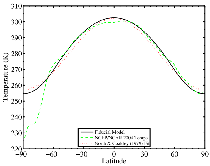
Figure 2: Model validation based on the mean latitudinal temperature profile of the Earth. The solid line shows the annual mean temperature profile in our fiducial Earth-like model. The dashed line shows the average taken from the NCEP/NCAR global temperature data in 2004. The dotted line shows the fit to Earth’s mean temperature profile proposed by North & Coakley (1979). The discrepancy at the South Pole is due to Antartica.

Figure 2 shows the annual mean temperature distribution in our fiducial model (solid line) after $130$ years of thermal relaxation. It is within 5 K of the phenomenalogical fit in Eq. (4), shown as a dotted line, at all latitudes. The model also reproduces quite well the zonally and temporally averaged surface temperatures from NCEP/NCAR for the year 2004 at all latitudes north of $60\arcdeg$ S. The North–South asymmetry of the land–distribution on Earth, due to the presence of a continental circumpolar region – Antarctica – in the south, breaks the symmetry of the temperature profile. It is therefore not surprising that our simple, symmetrical EBM fails to reproduce the sharply colder temperatures near the South Pole.

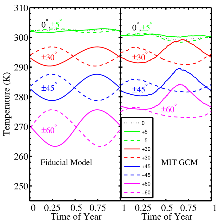
Figure 3: Model validation based on seasonality at different latitudes. The left panel shows temperatures as a function of time for several latitudes in our fiducial Earth-like model. The right panel shows the 2004 ocean–surface temperatures in the MIT Oceanic GCM (Wunsch & Hiembach, 2007) for the same latitudes. In both panels, solid lines correspond to temperatures in the North and dashed lines to temperatures in the South. Time of year is measured in fraction of a year from the northern winter solstice. Note that our model is North–South symmetrical while the MIT Oceanic GCM is not. Extrema of temperature occur approximately one quarter cycle after the extrema in forcing, as expected for a seasonally-forced planet in the limit of large thermal inertia (e.g., North & Coakley, 1979).

In addition to reproducing annual mean properties, the fiducial model also captures important seasonal variations seen in temperature data from the Earth or in advanced GCMs of the Earth. In particular, the temperature response is found to lag the solar forcing in our model by about a quarter annual cycle: the warmest temperatures happen at the local autumnal equinox and the coolest temperatuers at the local vernal equinox. This well known phase lag is the result of the high heat capacity of the wind-mixed ocean layer (e.g., North & Coakley (1979)), which covers 70% of our model Earth-like planet. For detailed comparison, we obtained surface layer outputs from the full three–dimensional MIT Oceanic GCM (Wunsch & Hiembach, 2007). Figure 3 shows the temperature as a function of time of year at latitudes from the equator to $\pm 60\arcdeg$, in our model and the uppermost ocean layer of the MIT GCM (5 m depth) for the year 2004. Time of year is measured in fraction of a year from the northern winter solstice. Our model is symmetrical with respect to the equator, so there is no real distinction between North and South, but the MIT GCM is not. Both models show the same response–lag of $\sim 90\arcdeg$. Towards the poles, our model gets significantly colder than the (ocean only) GCM, but at equatorial and mid–latitudes, remarkably, the deviations are in most places significantly less than 5 K.

Although our fiducial model is quite successful in reproducing various seasonal features of Earth’s temperature distribution, we caution that this alone does not guarantee that predictions will remain accurate for parameters other than the fiducial ones (e.g., for changes in orbital distance leading to systematically hotter or colder climates). To achieve a reasonably good fit to the Earth, various paramaters in the model were adjusted (e.g., constants in model 2 of Table 1 or value of $D_{\rm fid}$). Since the model is based on parameterizations, rather than fundamental laws, it is possible that its behavior will deviate quantitatively from what Earth’s response would be when new regimes of climate are explored. Nevertheless, the detailed model validation performed here with the Earth and the physics-based prescriptions adopted in our modeling strategy should guarantee that our EBM predictions are qualitatively robust. As we shall see below, this notion is supported by the generally good agreement of results obtained from the three different sets of atmospheric IR-cooling and albedo models listed in Table 1.

3 Study of Habitability

Equipped with a well-tested and validated EBM, we now reconsider several issues related to the habitability of Earth-like planets. In the present study, we emphasize differences between EBM and global radiative balance calculations, focusing on the concept of fractional habitability, and we highlight the potentially important role played by climate stability against snowball events in determining the habitability of an Earth-like planet.

3.1 Climate Dynamics and Seasonality

3.1.1 Climate Stability

Even a simple EBM such as ours can exhibit a surprisingly rich climate phenomenology, as compared to the outcomes of global radiative balance models. A particularly striking example of this phenomenology is the susceptibility of the climate system to albedo feedback effects that can induce transitions from partially ice–covered states to globally-frozen snowball states. In the context of habitability studies, these transitions are important because they could render a planet essentially “uninhabitable,” unless transitions back to partially ice–covered or ice–free states are possible. Since the seminal work of Budyko (1969) and Sellers (1969), it has been well known that Earth’s partially ice-covered climate allows for transitions to globally-frozen snowball states in response to relatively minor changes in forcings (e.g., Hartmann (1994); Ghil (2002); Hoffman & Schrag (2002)).

Climate stability is a subtle issue, even in the context of a 1D diffusion model. Held et al. (1981) describe how it is ultimately an interplay between latitudinal heat transport and albedo feedback effects that determines climate stability. Here, we will not attempt a thorough exploration of climate stability with our EBM but instead will illustrate how this issue could be critical in determining the habitability of a seasonally-forced Earth-like planet.

Latitudinal heat transport by atmospheric motions is inhibited by Coriolis effects on a rotating planet (e.g., Pedlosky (1982); Holton (1992)). As a result, latitudinal heat transport should be typically reduced on a pseudo-Earth rotating faster than the current Earth. There is currently no first principle theory allowing reliable estimates of how much transport would be reduced on a faster rotating Earth-like planet. There have been, however, simple scaling arguments proposed in the geophysical literature. Here, in the interest of simplicity, we will use the “thermal Rossby number” scaling advocated by Farrell (1990), which suggests that $D$ is $\propto{\Omega_{p}}^{-2}$, where $\Omega_{p}$ is the angular rotation rate of the planet (see also Stone 1973). We note that detailed GCM experiments for slow-rotating Earths do not necessarily support the extreme simplicity of the above scaling (del Genio et al., 1993; del Genio & Zhou, 1996).

Figure 4 shows space-time diagrams of temperature in two Earth-like models differing only in the magnitude of latitudinal heat transport. The top two panels show temperatures for the full 130 years (upper left) and for the last 5 years (upper right) of our fiducial Earth-like model. The bottom two panels show temperatures, over the same time spans, in a model of a pseudo-Earth that is in all respects identical to our fiducial model, except for a diffusion coefficient $D$ reduced by a factor of 9 (which, according to the above scaling, corresponds to a planet rotating three times as fast as Earth does). Both models start with a uniform $T=350$ K, but their evolutions follow strikingly different trajectories. The fiducial model settles to the standard, partially ice-covered solution. In contrast, the model with inefficient latitudinal heat transport undergoes rapid evolution through the first $\sim 50$ years, and then abruptly, over the course of a single year, transitions to a permanent snowball state with a mean temperature around 200 K.

Note that in the Earth–like fiducial model (upper right panel), the poles are, unsurprisingly, the coldest parts of the planet. By contrast, in the fast-Earth model (lower right panel), the poles become nearly as warm during local summer as the warmest parts of the planet. This is because, with our albedo function (model 2 in Table 1), the entire planet has identical albedo in the snowball state, and so the poles, which actually experience greater diurnally averaged insolation during local summer than any other part of the planet, can warm a great deal in response to the high solar irradiance. In the fiducial Earth-like model, on the other hand, parts of the planet that are above freezing absorb significantly more solar radiation, owing to their lesser albedo, than parts that are well below freezing; this is what keeps the poles relatively cold year–round in the fiducial model.

The main conclusion to be drawn from this comparison between our fiducial Earth-like model and a fast-rotating pseudo-Earth model is that issues of climate dynamics, especially climate stability with respect to snowball transitions, can critically influence the habitability of Pseudo–Earth planets. While the planetary rotation rate is simply inconsequential for global radiative balance models of habitability, it becomes a potentially important planetary attribute for habitability in more elaborate dynamical climate models, even for Earth-like planets at $1$ AU from a Sun-like star, as was assumed in both models shown in Figure 4.

3.1.2 Comparison to Global Radiative Balance Results

We now relax our $1$ AU assumption and calculate EBMs for Earth-like planets at a range of orbital distances from their Sun-like star. We place our model planets at $41$ distances from the star, in the range $0.3$ to $1.3$ AU, with $0.025$ AU steps. Each model is run for $130$ local years (orbits), which is sufficient for adequate model relaxation from the hot-start to the final periodic climate solution. At every distance, we also calculate the radiative equilibrium temperature that obtains from the global average insolation, so that we can directly compare our time-dependent EBM results to those of an equivalent global radiative balance model.

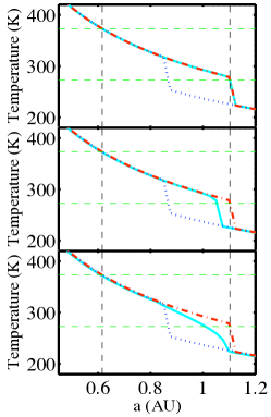
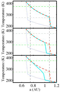
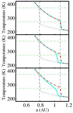
Figure 5: Comparison between global radiative equilibrium temperatures and averaged temperatures in our seasonal EBM, for nine different pseudo-Earth models. From left to right, the three columns show results obtained using models 1, 2 and 3 in Table 1 for the IR-cooling and albedo functions, respectively. In each column, from top to bottom, panels correspond to values $D=9\,D_{\rm fid}$, $D_{\rm fid}$, and $D_{\rm fid}/9$ for the latitudinal diffusion coefficient used in the EBM. In each panel, the solid curve shows the global and annual mean temperature in the EBM over a range of orbital distances. The dotted and dashed-dotted curves show the corresponding low- and high-temperature radiative equilibrium solutions, respectively. The mean temperature in the EBM deviates from the high-temperature radiative equilibrium solution for small and moderate values of the coefficient of latitudinal heat diffusion.

As discussed in § 2.1, there is in general a range of orbital distances around $\sim 1$ AU for which multiple radiative equilibrium solutions exist. We focus exclusively on the two stable, low and high temperature solutions here. Each panel in Figure 5 compares the radiative equilibrium solutions (dotted and dashed-dotted curves) to results for the annual mean temperature weighted by surface area in our EBM calculations (solid line), for a range of orbital distances. From left to right, the three columns show results using models 1, 2, and 3 in Table 1, respectively, for the IR-cooling and albedo functions. In each column, EBM results are shown for three efficiencies of latitudinal heat transport, corresponding to $D=9\,D_{\rm fid}$, $D_{\rm fid}$, and $D_{\rm fid}/9$, from top to bottom. Our fiducial Earth-like model corresponds to the central panel.

At small and large orbital separations, the EBM and radiative-balance curves nearly coincide with each other, indicating that the unique radiative equilibrium solution is very close to the averaged temperature in our seasonal EBM. At intermediate separations corresponding to partially ice-covered climates, however, the curves separate. The distinction among the three curves is particularly important for EBMs with weak latitudinal heat transport (bottom panels) because EBMs with efficient latitudinal heat transport (top panels) have generally more uniform temperature distributions, which is close to the implicit averaging assumption made in global radiative balance models.

Each panel in Figure 5 has horizontal dashed lines at 273 K (water freezing) and at 373 K (water boiling) and vertical dashed lines indicating where the high temperature radiative equilibrium solution crosses these 273 K and 373 K limits. In other words, the vertical dashed lines indicate the orbital extent of the radiative equilibrium habitable zone (hereafter, REHZ) for globally averaged conditions, analogous to the calculations in Kasting et al. (1993). The extent of the habitable zone defined on the basis of the globally and annually averaged temperature in our EBMs is the range of orbital radii, $a$, for which the solid curve remains between the two horizontal dashed lines (indicating surface liquid water conditions for an Earth-like planet). In all the models considered here, this EBM-average habitable zone tends to have nearly the same inner boundary as the REHZ, but its outer boundary can be significantly closer to the Sun-like star than that of the REHZ. Indeed, in EBMs with fiducial or reduced efficiencies of latitudinal heat transport, the climate typically makes dynamical transitions to a fully ice-covered snowball state at orbital distances well inside of what global radiative balance models might indicate. Although quantitative discrepancies exist, this qualitative behavior is common to all three models with different IR-cooling and albedo functions shown in Fig. 5. Note that the dynamical transition to a snowball state shown in Fig. 4 for a fast-rotating pseudo-Earth at $1$ AU is included in the lower middle panel of Fig. 5.

While useful for comparisons between EBM and global radiative balance results, the diagrams shown in Fig. 5 do not accurately capture the range of surface temperature conditions found in our seasonal EBMs. Indeed, for every globally averaged annual mean temperature from an EBM, there must exist a range of temperatures above and below this average, both in a regional and a temporal sense. In general, planets can therefore be habitable beyond what globally averaged studies might indicate. This leads us to give a formal definition of the notion of fractional habitability.

3.2 Fractional Habitability

For a fixed set of forcing and response parameters, a planet might be habitable (i.e., have a surface temperature between 273 K and 373 K) over only a portion of its total surface area or for only a fraction of its orbit. To quantify the various possible outcomes in our EBMs, we develop several metrics of fractional habitability.

Let $H[a,\lambda,t]$ be the “habitability function”, equal to 1 if latitude $\lambda$, on a model planet at a distance $a$ from its star, has a habitable temperature at time $t$, and 0 otherwise:

$$H[a,\lambda,t]=\left\{\begin{array}[]{ll}1&{\rm if}\,273\leq T[a,\lambda,t]\leq 373,\\ 0&{\rm otherwise.}\end{array}\right..$$ (5)

Using $H$, we define three habitability fractions.

At each latitude, we calculate the fraction of the year that that portion of the planet spends in the habitable temperature range,

$$f_{\rm time}[a,\lambda]=\frac{\int_{t=0}^{P}H[a,\lambda,t]dt}{P},$$ (6)

where $f_{\rm time}$ is the habitable fraction as a function of latitude, and $P$ is the length of the year at orbital separation $a$. At each time of year, we calculate the fraction of the planet’s surface area that is habitable:

$$f_{\rm area}[a,t]=\frac{\int_{\lambda=-\pi/2}^{\pi/2}H[a,\lambda,t]\cos[\lambda]d\lambda}{2}.$$ (7)

Finally, at each orbital separation, we calculate the net fractional habitability, which is the area–weighted fraction of the $\lambda-t$ plane over which the planet is habitable:

$$f_{\rm hab}[a]=\frac{\int_{\lambda=-\pi/2}^{\pi/2}\left\{\int_{t=0}^{P}H[a,\lambda,t]dt\right\}\cos[\lambda]d\lambda}{2P}.$$ (8)

3.2.1 The Case of Earth

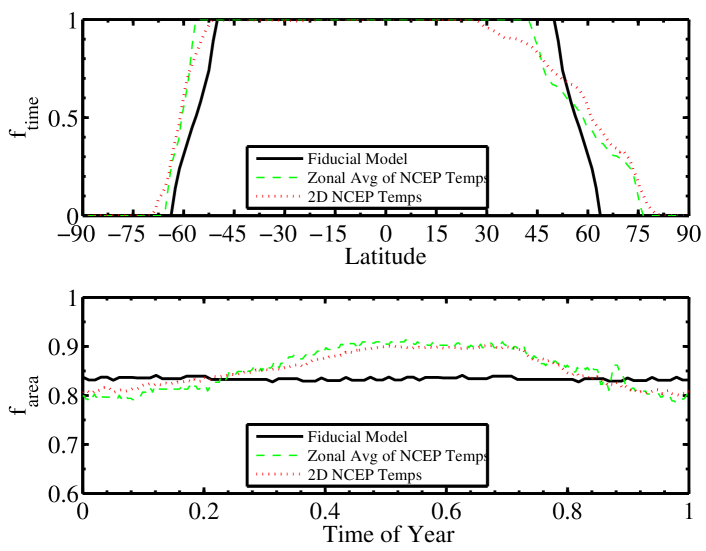
Figure 6: Temporal and regional habitability fractions of the Earth and in our fiducial Earth-like model. The top panel shows $f_{\rm time}$, the fraction of the time that each latitude band spends between 273 K and 373 K. The bottom panel shows $f_{\rm area}$, the fraction of the land area that is between 273 K and 373 K at different times of year, measured from the Northern winter solstice. In both panels, the solid line shows results for our fiducial model, the dashed line shows results for the Earth using the zonally-averaged NCEP/NCAR temperature data in 2004, and the dotted line shows results for the Earth using the full two–dimensional NCEP/NCAR 2004 temperature data.

Before analyzing the fractional habitability of model planets with different characteristics than Earth, it is instructive to consider the fractional habitability of Earth itself and of our fiducial Earth-like model. We return to the NCEP/NCAR temperature data in 2004 for this comparison. Figure 6 shows a remarkably good agreement between the temporal and regional habitability of our fiducial model (solid line) and that of Earth (dashed and dotted lines). We analyzed the 2004 Earth temperatures in two different ways. In order to create a variable that is directly comparable to our (one dimensional) model temperatures, we must perform zonal averages. In Figure 6, statistics derived from first zonally-averaged temperatures are represented by dashed lines. We also used the entire data set (latitude, longitude and time) to calculate habitability fractions before performing zonal averages. Statistics derived from this full set of temperature data are represented by dotted lines.

The top panel in Figure 6 shows the fraction of the time that each latitude strip spends at or above 273 K. There are some differences between the dashed and the dotted lines, most noticeably in the steepness of the descent from 100% habitable to 0% habitable moving from equator to North Pole. The crucial feature of this plot, from a model validation perspective, is that the $f_{\rm time}$ values derived from zonally averaged temperatures on Earth have a very steep descent in both hemispheres, similar to what is seen in our fiducial model.

The bottom panel in Figure 6 shows the fraction of the surface area that is habitable as a function of time of year (measured from the Northern winter solstice). The fiducial model maintains nearly constant regional habitability throughout the year. Earth’s regional habitability varies slightly over the year, increasing a bit in the Northern summer because the North Polar ice cap shrinks much more during its summer than the South Polar cap does during its.

Finally, the net fractional habitability ($f_{\rm hab}$) of Earth and of our fiducial model are just the average values of the curves shown in the bottom panel of Figure 6. Our fiducial model is 83% habitable. Earth was 85% habitable in 2004 when calculated from two–dimensional temperature data (this fraction varies by less than 0.5% from year to year). The net fractional habitability of Earth was 86% in 2004 when calculated from a temperature field that is first zonally averaged.

3.2.2 Temporal Habitability of Pseudo-Earths

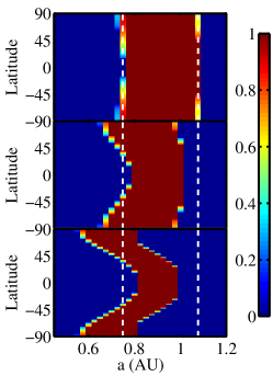
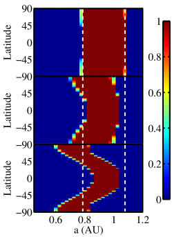
Figure 7: Temporal habitability fraction, $f_{\rm time}$, as a function of orbital distance and latitude. Results are shown for the same nine pseudo-Earth models as in Fig. 5, with the same panel structure. Vertical dashed lines indicate the orbital extent of the radiative equilibrium habitable zone. Fractional habitability increasingly depends on latitude, and deviates from radiative equilibrium results, when the efficiency of latitudinal heat transport ($D$) is reduced (from top to bottom).

Figure 7 presents a striking view of how regionality depends on the efficiency of latitudinal heat transport with the same nine pseudo-Earth EBMs as shown in Fig. 5. In this figure, contours indicate the value of the temporal habitability, $f_{\rm time}$, as a function of orbital separation ($a$) and latitude ($\lambda$). When latitudinal heat transport is efficient – in the top panels – temporal habitability depends little on latitude. When transport is inefficient – in the bottom panels – there is a great deal of latitudinal dependence. Since the poles tend to be colder at a given separation, they tend to be habitable when the planet is closer to the star. For the same reason, the equator tends to be habitable when the planet is further away from the star.

In each panel, the dashed vertical lines indicate the orbital extent of the radiative equilibrium habitable zone (REHZ), taken from Figure 5. In all models, allowing for regionality extends the inner boundary of the habitable zone, relative to the REHZ. Models with low efficiencies of latitudinal heat transport tend to have outer boundaries of the habitable zone that are closer to the star than models with high $D$ values. In essentially all cases, this outer boundary is determined by a dynamical climate transition to a globally-frozen snowball state. As a result, the relationship between the outer boundary of the regionally habitable zone and $D$ is not necessarily monotonic. In the left column of Figure 7, for example, the outer boundary of the regionally habitable zone is minimum for $D=D_{\rm fid}$. In all models, at a given latitude, planets tend to be habitable either 100% of the time or 0% of the time, with little space for intermediate cases. As we shall see below, this is a consequence of the assumed large ocean fraction (70%) on the model planets. The large resulting thermal inertia minimizes the ability of a latitude band to swing below and above the freezing point during an annual cycle.

One may ask what is the physical process that actually drives a model planet to freeze over into a snowball state at a given orbital separation. For instance, in the central panel of Figure 7, which shows results for our fiducial Earth-like model, the planet has an Earth–like climate at $a=1$ AU but is globally-frozen at $a=1.025$ AU. What is different at 1.025 AU than at 1.000 AU to induce such a dynamical transition? Two possibilities spring to mind: the reduced insolation or the longer winters. In order to distinguish between these two possibilities, we ran two additional models: one with Earth–like insolation and a year longer by a factor of $1.025^{3/2}$ (which did not freeze), and one with insolation reduced by a factor of $1.025^{2}$ and a year the length of Earth’s (which did freeze). This indicates that the reduced insolation is the dominant effect leading to snowball transitions in this model. As shown explicitly in Appendix II, however, longer winters can also contribute to dynamical snowball transitions.

3.2.3 Regional Habitability of Pseudo-Earths

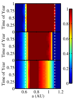
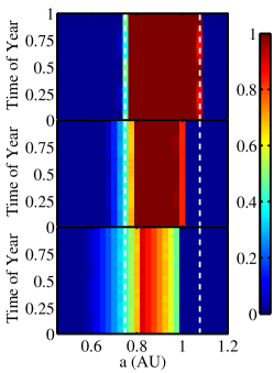
Figure 8: Regional habitability fraction, $f_{\rm area}$, as function of orbital distance and time of year. Results are shown for the same nine pseudo-Earth models as in Fig. 5, with the same panel structure. Vertical dashed lines indicate the orbital extent of the radiative equilibrium habitable zone. In models with efficient latitudinal heat transport (top row), the regional habitability fraction tends to be either 0 or 1. In low transport efficiency models (bottom row), the regional habitability fraction takes on more intermediate values.

Figure 8 shows temporal variation in fractional habitability for the same nine pseudo-Earth EBMs as before. In this figure, contours indicate the value of the regional habitability, $f_{\rm area}$, as a function of orbital separation and time of year. As before, time of year is measured in fraction of a year from the northern winter solstice. There is little temporal variability in the nine models shown. This is a consequence of the North–South symmetry and the large thermal inertia of these models, with $70$% ocean fraction. A model with North–South asymmetry in the distribution of land and sea, or even a symmetrical model with a much reduced ocean fraction, would show more significant variations in the value of $f_{\rm area}$ with time.

In models with efficient latitudinal heat transport (top panels), $f_{\rm area}$ tends to be either 0 or 1, taking on intermediate values only over a very small range of orbital separations. This is a consequence of the latitudinal isothermality of these models: essentiall the entire planetary surface is either above 273 K or below it. By contrast, models with inefficient latitudinal heat transport (bottom panels) are habitable over 100% of the planetary surface area only in a small portion of the regionally habitable zone. In fact, models shown in the lower middle and lower right panels are never habitable over the entire surface area of the planet.

3.2.4 Pseudo-Earth with a Small Ocean Fraction

The presence of abundant oceans on Earth plays a critical role in regulating its climate, but there is no fundamental reason why a terrestrial planet should have Earth–like ocean covering. The heat capacity $C$ in equation (3) has units of $\rm[time]\times[energy\,flux]/[temperature]$. Multiplying $C$ by a characteristic temperature and dividing by a characteristic flux, therefore, provides an estimate of the characteristic timescale for thermal relaxation:

$$t_{\rm relax}\sim\frac{C\times\bar{T}}{(S/4)\times(1-\bar{A})}.$$ (9)

For Earth–like conditions, using $T\sim 300$ K, $S\sim 1.4\times 10^{6}{\rm~{}erg~{}cm^{-2}~{}s^{-1}}$, and $\bar{A}\sim 0.5$, we find

$$t^{\rm E}_{\rm relax}\sim\frac{0.0017{\rm~{}K}}{1{\rm~{}erg~{}cm^{-2}}}C{\rm~{}s}.$$ (10)

In our EBM, we assign to the atmosphere a heat capacity that accounts for the type of (thermally coupled) surface that lies beneath it. Since the atmospheric heat capacity over land in our EBM is $C_{l}=5.25\times 10^{9}{\rm erg~{}cm^{-2}~{}K^{-1}}$, the corresponding relaxation timescale is roughly $t^{\rm E,l}_{\rm relax}\sim 9\times 10^{6}{\rm~{}s}$, or about 0.3 years – between 3 and 4 months. On the other hand, the atmospheric heat capacity over ocean is 40 times larger because the atmosphere is able to tap into the larger thermal inertia of a mixed–wind layer at the ocean’s surface. This results in a relaxation timescale $t^{\rm E,o}_{\rm relax}$ over ocean that is slightly longer than 10 years in our models. Consequently, in any EBM of a planet that is more than one part in 40 (2.5%) uniformly covered by ocean, the thermal relaxation timescale is approximately given by the ocean relaxation timescale times the ocean fraction.

The pseudo-Earth EBMs presented so far, all with a uniform 70% ocean fraction, have long thermal timescales of nearly a decade ($\sim 8$ years). By contrast, a model planet with only a 10% ocean fraction would have a thermal timescale that is closer to a year. In such a model, one would expect significantly larger seasonal variations in temperature over the course of a year.

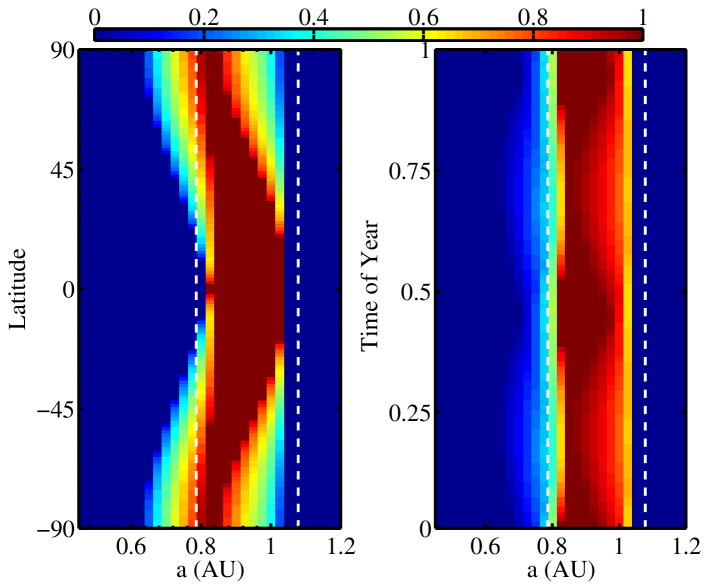
Figure 9: Temporal and regional habitability fractions in a pseudo-Earth model with a uniform 10% ocean fraction. The model is in every way similar to our fiducial Earth-like model, except for the reduced ocean fraction. The left panel shows the temporal habitability, $f_{\rm time}$, as a function of orbital distance and latitude. The right panel shows the regional habitability, $f_{\rm area}$, as a function of orbital distance and time of year. In each panel, vertical dashed lines indicate the orbital extent of the radiative equilibrium habitable zone. With this smaller ocean fraction, the temporal habitability (left panel) takes on more intermediate values (between 0 and 1) and the regional habitability (right panel) shows seasonal variations with time of year (two cycles per year because of the North–South model symmetry).

Figure 9 shows temporal and regional habitability diagrams for a pseudo-Earth EBM that is identical to our fiducial Earth-like model, except for a uniform ocean fraction reduced from 70% to 10%. The left panel shows the temporal habitability, $f_{\rm time}$, as a function of orbital distance and latitude, while the right panel shows the regional habitability, $f_{\rm area}$, as a function of orbital distance and time of year (measured in fraction of a year from the solstice). In contrast to the fiducial model with 70% ocean fraction shown in the central panels of Figures 7 and 8, there are now large swaths of parameter space, both in the left and right panels, that take on habitability fractions between 0 and 1. Seasonal variations of the regional habitability fraction are easily identified in the right panel, with two “seasonal cycles” per year from the North–South symmetry of the model. Note that the range of orbital distances with nonzero fractional habitability, for this drier pseudo-Earth, differs only slightly from the corresponding range in the fiducial Earth–like model with $70$% ocean fraction, with an outer edge somewhat extended.

Table 2 summarizes the different sizes of fractionally habitable zones for the various models considered in this study. Compared to global radiative balance calculations, fractionally habitable zones extend closer to the star, simply as a result of the range of regional conditions that obtain on the planet in our EBMs. On the other hand, the outer reach of fractionally habitable zones tends to be limited, before the outer radiative limit is reached, by dynamical climate transitions to globally-frozen snowball states. Planetary rotation rates and land-ocean fractions influence the orbital extent of fractionally habitable zones. Since these and other relevant planetary attributes will be unknown for terrestrial exoplanets, assessments of habitability for these newly discovered worlds will be complicated by these uncertainties.

4 On the Definition of Habitability

Determining the habitable zone of model or actual planets is an interdisciplinary endeavor that requires the contributions of biologists, climatologists, and astronomers. In light of our results on the rich phenomenology of habitable climates, we find it useful to mention here a few qualitative points that may prove to be important in refining the notion of habitability beyond the standard orbital radius requirement for surface liquid–water generally discussed in the astronomical literature (e.g., Kasting et al. 1993).

Habitability on Earth is not strictly tied to the freezing point of water. Carpenter et al. (2000) have discovered bacterial activity in South Pole snow, indicating that some organisms can reproduce at ambient temperatures below $-10\arcdeg$ C and can live at temperatures down to $-85\arcdeg$ C. Nor is habitability strictly tied to the sea–level boiling point of water on Earth. Kashefi & Lovley (2003) have cultured a strain of archaea that happily reproduces at $121\arcdeg$ C, and remains viable at temperatures up to at least $130\arcdeg$ C. The idea that life requires temperatures appropriate for liquid water at 1 Atm pressure is therefore at least partially flawed. These examples would indicate that the habitable temperature range ought to be extended to 263 K–394 K, or even possibly 188 K–403 K. Biologists will have the final say on three vital ranges of temperature, by determining when life can arise, survive and reproduce. The temperature regime in which organisms can reproduce may be the relevant one for the definition of habitability in the context of astronomical searches.

Even if life requires liquid water, one must still carefully consider the upper temperature limit to habitability. Water boils at 373 K only for a surface pressure of 1 Atm. There is so much water in the Earth’s oceans that the surface temperature could be well above 373 K and the atmospheric H₂O pressure change could allow liquid water to remain on the surface. On the other hand, since water is a greenhouse gas and humidity increases with temperature, a planet’s ability to cool is likely to become significantly reduced at some critical temperature. Unless additional feedbacks intervene at these high temperatures, such as higher albedo from increased cloud coverage, a regime of “runaway greenhouse effect” may be reached. Kasting (1988) and Sugiyama et al. (2005) have argued that this runaway regime would be reached for global surface temperatures between $\sim 350$ K and $\sim 400$ K on Earth. These important considerations, which have not been addressed in our modeling strategy, suggest that the high–temperature end of the habitable range may be the critical temperature for runaway greenhouse effect, at least for Earth-like planets.

We note, however, that all these notions should also be fully integrated with the regional and seasonal character of climate systems. Mean planetary conditions do not necessarily determine the ability of a planet to host life. Rather, the various conditions achieved on different parts of the planet, at different times of year, do. Knowning mean conditions is useful only insofar as they are a good proxy for actual local conditions, but in many cases they may not be. Allowing for seasonality renders concepts such as the runaway greenhouse effect significantly more complicated. For example, if parts of a planet (e.g., equatorial regions) are above the critical temperature for runaway greenhouse effect, while other parts (e.g., polar regions) are not, determining whether or not the planet’s temperature does run away becomes a non-trivially coupled problem.

Finally, we note that in order for a planet to be considered habitable, it may need attributes such as its net fractional habitability, $f_{\rm hab}$, to exceed some minimum threshold values. For one thing, this may be required for life to arise and survive on the planet. But such a requirement may also be important in terms of observational searches for biomarkers and other signatures of life. If only a small fraction of the planet’s surface area is habitable, or if it is habitable only for a small fraction of the year, the planet may host life but this life may be unable to generate large enough signatures – e.g., in spectral biomarkers (Kaltenegger & Selsis, 2007; Kiang et al., 2007; Grenfell et al., 2007; Seager et al., 2005) – to permit reliable detections with specific remote sensing instruments. Understanding the minimum fractional habitability necessary to produce sufficient atmospheric concentrations of biomarkers detectable by instruments such as TPF and Darwin will be an interesting challenge for the emerging field of astrobiology.

5 Conclusion

We have reconsidered the notion of habitability for Earth-like planets with seasonal energy-balance climate models. These models show that the concept of regional and seasonal habitability is generally important to assess the ability of terrestrial exoplanets to host life. We find that previous evaluations of habitable zones may have omitted important climatic conditions by focusing on close Earth analogies. We illustrate this with two specific examples: pseudo–Earths rotating at different rates or possessing a smaller ocean fraction than Earth itself. These pseudo-Earths have quantitatively different climatic habitability properties than the Earth itself.

Comparisons to global radiative balance calculations show that seasonal habitability generally extends the inner orbital range of Earth-like planet habitable zones. The outer orbital range is reduced relative to what global radiative balance calculations would indicate, however, because the climate generally makes a dynamical transition to a globally-frozen snowball state before the outer radiative limit is reached. The stability of a planet’s climate against snowball events therefore has a strong impact on its habitability. Since this stability is partly determined by external forcing factors such as the magnitude of insolation and the length of winters, we expect issues of climate dynamics to be central in determining the habitability of terrestrial exoplanets, particularly if their forcing conditions are generally different from the moderate cases encountered in the Solar System.

APPENDIX

In this appendix, we describe several numerical tests developed in the process of building our EBMs. We discuss the importance of sufficient spatial resolution for converged results and the effects that initial conditions have in determining the final periodic climate solutions obtained.

I Numerical Resolution

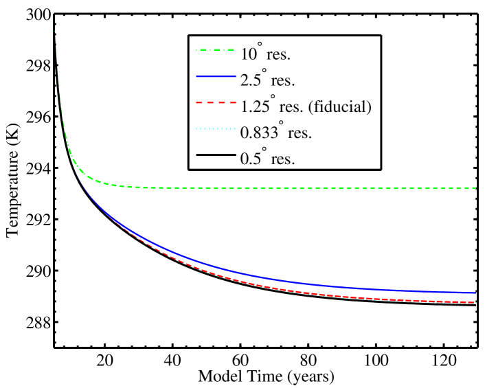
Figure 10: Numerical convergence tests. The global mean temperature in our fiducial Earth-like model is shown, convolved with a 1–year boxcar filter, for five different numerical resolutions. From top to bottom, the resolution is $10\arcdeg$ on the sphere (19 latitudinal grid points), $2.5\arcdeg$ (73 points), $1.25\arcdeg$ (145 points), $0.833\arcdeg$ (217 points), and $0.5\arcdeg$ (361 points). The default resolution adopted in our work is $1.25\arcdeg$.

We investigated numerical resolution issues with a hot–start version of our reference Earth-like model. It has uniform initial temperature $T=350{\rm~{}K}$, uses “model 2” formulations for the IR-cooling and albedo functions (see Table 1) and adopts the fiducial value $D=D_{\rm fid}$ for the magnitude of latitudinal heat transport. Here, we describe the results of a convergence test for five spatial resolutions: $10\arcdeg$ on the sphere (19 grid points equally spaced in latitude, including the poles); $2.5\arcdeg$ (73 points); $1.25\arcdeg$ (145 points); $0.833\arcdeg$ (217 points); and $0.5\arcdeg$ (361 points; the “high resolution model”). Figure 10 shows the time evolution of the global mean surface temperature in the same Earth-like models at different numerical resolutions. Small-amplitude annual oscillations in the global mean temperature have been smoothed out by convolving each temperature time series with a 1–year boxcar filter.

As the numerical resolution is increased, differences between the global temperature relaxation curves diminish rapidly, as expected from the second-order spatial differencing scheme used. After 130 years, the model with $2.5\arcdeg$ resolution achieves a periodic solution for the global mean temperature that is within $\sim 0.5{\rm~{}K}$ of the solution with the high resolution model. The $1.25\arcdeg$ resolution model stays within 0.2 K of the high resolution model and the $0.833\arcdeg$ resolution model is barely distinguishable from the high resolution model (within $0.1$ K). To strike a good balance between numerical accuracy and integration speed, we adopt a $1.25\arcdeg$ resolution in all our models. This guarantees that our results are not significantly affected by finite resolution effects. With this level of numerical accuracy, it is clear that the simplicity of various assumptions in our modeling strategy will be the key factor limiting the predictive power of our EBMs.

We note that the model with $10\arcdeg$ resolution relaxes to a periodic solution much faster than the other models and that it settles to a global mean temperature that deviates from the higher resolution results by more than $4$ K. This consequence of poor numerical resolution may be important since several EBM studies have been carried out in the past at this standard $10\arcdeg$ resolution (e.g., Sellers (1969), WK97). Traditionally, one of the main justifications for using such a low spatial resolution is that the diffusive model for latitudinal heat transport is not expected to provide a reliable description of much smaller spatial scales given an Earth-like circulation regime (e.g., Lorenz (1979); North & Coakley (1979)). It is our opinion, however, that it is preferable to reach satisfactory numerical convergence with the diffusive model even if the model itself is not be used to interpret phenomena below some intermediate scale effectively exceeding the numerical resolution. Otherwise, even global results like the mean surface temperature shown in Fig. 10 may be prone to finite resolution effects. This becomes particularly important in the context of climate dynamical studies where slight differences in model attributes, such as initial conditions, can have a profound influence on the ultimate outcome for the climate, as we shall now illustrate.

II Initial Conditions

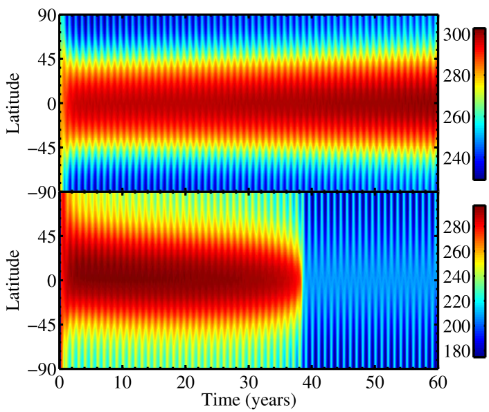
Figure 11: Dependence on initial conditions (orbital time). Both panels show space-time diagrams of temperature in our fiducial Earth-like model starting with a uniform temperature of $275$ K. The model in the top panel begins at the Northern winter solstice and it recovers from the rather cool initial condition by asymptotically approaching the same partially ice-covered climate solution as for typical hot–start cases. The model in the bottom panel, however, begins at the Northern vernal equinox and makes a dynamical transition to a globally-frozen snowball state after approximately 38 years.

Repeated experiments with our reference Earth-like EBM show that, as long as the uniform initial temperature is chosen to be far above $273$ K, essentially all memory of the initial conditions is lost by 130 years of evolution. For initial temperatures approaching $273$ K, however, there can be very sensitive dependence on the initial conditions, due to strong water-ice albedo feedback effects. Here we show that even for the same initial conditions in temperature, different outcomes for the climate are possible depending on the time of year at which the model is started. Figure 11 shows space-time diagrams of temperature in two models which are identical in all respects, including a uniform initial $T=275{\rm~{}K}$, except for the initial time on the orbit. The model in the top panel begins with the $23.5$°-obliquity planet at the northern winter solstice while the one in the bottom panel begins at the northern vernal equinox (a quarter year later). After 60 years, the model in the top panel is still evolving, but it is clearly making its way to the same periodic, partially ice-covered solution as in the top panels of Figure 4. The model in the bottom panel, on the other hand, transitions to a fully ice-covered snowball state after slightly less than 40 years. The North–South asymmetry evident in the bottom panel shows that the model never lost memory of its unbalanced start. The model’s northern hemisphere started in the spring, and therefore experienced 6 months of greater insolation than the southern hemisphere, from the very beginning. As a result, the southern hemisphere remained significantly, and increasingly, colder than the northern hemisphere, until the cold temperatures in the south were able to drag the entire planet down to a globally-frozen snowball state.

Table 1: Atmospheric Models

Model	IR Cooling Function	Albedo Function
1	$I_{1}[T]=\frac{\sigma T^{4}}{1+(3/4)\tau^{0}_{\rm IR}}$	$A_{1}[T]=0.5-0.2\tanh[\frac{(T-268{\rm K})}{5{\rm K}}]$
2	$I_{2}[T]=\frac{\sigma T^{4}}{1+(3/4)\tau_{\rm IR}[T]}$	$A_{2}[T]=0.525-0.245\tanh[\frac{(T-268{\rm K})}{5{\rm K}}]$
3	$I_{3}[T]=A+BT$	$A_{3}[T]=0.475-0.225\tanh[\frac{(T-268{\rm K})}{5{\rm K}}]$

Note. — $\sigma$ is the Stefan-Boltzmann constant.

Table 2: Habitable Zone Extents

Table 1 Model:	# 1	# 2	#3
Global Radiative Balance	0.616-1.103	0.748-1.077	0.786-1.078
EBM with $D=9D_{\rm fid}$	0.550-1.125	0.700-1.100	0.750-1.100
EBM with $D=D_{\rm fid}$	0.450-1.075	0.625-1.025	0.675-1.050
EBM with $D=(1/9)D_{\rm fid}$	0.400-1.100	0.525-1.000	0.575-1.050
EBM with 10% ocean fraction	–	0.625-1.050	–

Note. — Habitable zones in each of the models considered. All orbital distances are in AU.

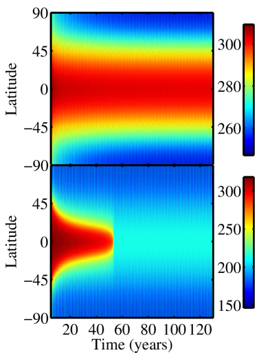
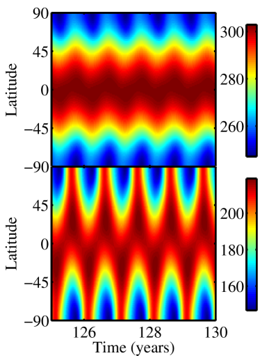
Figure 4: Space-time diagrams of temperature (in K) for two different pseudo-Earth models. Left panels show the entire 130 years of evolution while the right panels show only the last 5 years of seasonal climate. The top two panels show the evolution of temperatures in our fiducial Earth-like model. The bottom two panels show the evolution of temperatures in a pseudo-Earth model that is identical to the fiducial model, except for a coefficient of latitudinal heat transport reduced by a factor of 9 from the fiducial value ($D_{\rm fid}/9$). A reduced efficiency of latitudinal heat transport is expected on fast-rotating pseudo-Earths. The model with inefficient latitudinal heat transport makes a dynamical transition to a globally-frozen snowball state after approximately $50$ years.

References

- Adams et al. (2007) Adams, E. R., Seager, S., & Elkins-Tanton, L. 2007, ArXiv e-prints, 710
- Baglin (2003) Baglin, A. 2003, Advances in Space Research, 31, 345
- Barnes (2007) Barnes, J. W. 2007, PASP, 119, 986
- Basri et al. (2005) Basri, G., Borucki, W. J., & Koch, D. 2005, New Astronomy Review, 49, 478
- Baum & Crowley (2003) Baum, S. K. & Crowley, T. J. 2003, Geophys. Res. Lett., 30, 1
- Beaulieu et al. (2006) Beaulieu, J.-P., Bennett, D. P., Fouqué, P., Williams, A., Dominik, M., Jorgensen, U. G., Kubas, D., Cassan, A., Coutures, C., Greenhill, J., Hill, K., Menzies, J., Sackett, P. D., Albrow, M., Brillant, S., Caldwell, J. A. R., Calitz, J. J., Cook, K. H., Corrales, E., Desort, M., Dieters, S., Dominis, D., Donatowicz, J., Hoffman, M., Kane, S., Marquette, J.-B., Martin, R., Meintjes, P., Pollard, K., Sahu, K., Vinter, C., Wambsganss, J., Woller, K., Horne, K., Steele, I., Bramich, D. M., Burgdorf, M., Snodgrass, C., Bode, M., Udalski, A., Szymański, M. K., Kubiak, M., Wiȩckowski, T., Pietrzyński, G., Soszyński, I., Szewczyk, O., Wyrzykowski, Ł., Paczyński, B., Abe, F., Bond, I. A., Britton, T. R., Gilmore, A. C., Hearnshaw, J. B., Itow, Y., Kamiya, K., Kilmartin, P. M., Korpela, A. V., Masuda, K., Matsubara, Y., Motomura, M., Muraki, Y., Nakamura, S., Okada, C., Ohnishi, K., Rattenbury, N. J., Sako, T., Sato, S., Sasaki, M., Sekiguchi, T., Sullivan, D. J., Tristram, P. J., Yock, P. C. M., & Yoshioka, T. 2006, Nature, 439, 437
- Borucki et al. (2003) Borucki, W. J., Koch, D., Basri, G., Brown, T., Caldwell, D., Devore, E., Dunham, E., Gautier, T., Geary, J., Gilliland, R., Gould, A., Howell, S., & Jenkins, J. 2003, in ESA Special Publication, Vol. 539, Earths: DARWIN/TPF and the Search for Extrasolar Terrestrial Planets, ed. M. Fridlund, T. Henning, & H. Lacoste, 69–81
- Borucki et al. (2007) Borucki, W. J., Koch, D. G., Lissauer, J., Basri, G., Brown, T., Caldwell, D. A., Jenkins, J. M., Caldwell, J. J., Christensen-Dalsgaard, J., Cochran, W. D., Dunham, E. W., Gautier, T. N., Geary, J. C., Latham, D., Sasselov, D., Gilliland, R. L., Howell, S., Monet, D. G., & Batalha, N. 2007, in Astronomical Society of the Pacific Conference Series, Vol. 366, Transiting Extrapolar Planets Workshop, ed. C. Afonso, D. Weldrake, & T. Henning, 309–+
- Budyko (1969) Budyko, M. I. 1969, Tellus, 21, 611
- Canup (2004) Canup, R. M. 2004, Icarus, 168, 433
- Carpenter et al. (2000) Carpenter, E. J., Lin, S., & Capone, D. G. 2000, Applied and Environmental Microbiology, 66, 4514
- del Genio & Zhou (1996) del Genio, A. D. & Zhou, W. 1996, Icarus, 120, 332
- del Genio et al. (1993) del Genio, A. D., Zhou, W., & Eichler, T. P. 1993, Icarus, 101, 1
- Dole (1964) Dole, S. H. 1964, Habitable planets for man (New York, Blaisdell Pub. Co. [1964] [1st ed.].)
- Farrell (1990) Farrell, B. F. 1990, Journal of Atmospheric Sciences, 47, 2986
- Firsoff (1963) Firsoff, V. A. 1963, Life beyond the earth; a study in exobiology. (New York, Basic Books [1964, c1963])
- Ford et al. (2008) Ford, E. B., Quinn, S. N., & Veras, D. 2008, ArXiv e-prints, 801
- Forget & Pierrehumbert (1997) Forget, F. & Pierrehumbert, R. T. 1997, Science, 278, 1273
- Fortney et al. (2007) Fortney, J. J., Marley, M. S., & Barnes, J. W. 2007, ApJ, 659, 1661
- Franck et al. (2000) Franck, S., von Bloh, W., Bounama, C., Steffen, M., Schönberner, D., & Schellnhuber, H.-J. 2000, J. Geophys. Res., 105, 1651
- Gaidos et al. (2005) Gaidos, E., Deschenes, B., Dundon, L., Fagan, K., Menviel-Hessler, L., Moskovitz, N., & Workman, M. 2005, Astrobiology, 5, 100
- Gaidos & Williams (2004) Gaidos, E. & Williams, D. M. 2004, New Astronomy, 10, 67
- Ghil (2002) Ghil, M. 2002, Encyclopedia of Atmospheric Sciences, J. R. Holton, J. Pyle, and J. A. Curry (Eds.), 432
- Goldsmith & Owen (2002) Goldsmith, D. & Owen, T. 2002, The Search for Life in the Universe (Sausalito, CA, University Science Books [2002] [3rd ed.].)
- Grenfell et al. (2007) Grenfell, J. L., Stracke, B., von Paris, P., Patzer, B., Titz, R., Segura, A., & Rauer, H. 2007, Planet. Space Sci., 55, 661
- Haldene (1954) Haldene, J. B. S. 1954, New Biology, 16
- Hameury et al. (1998) Hameury, J.-M., Menou, K., Dubus, G., Lasota, J.-P., & Hure, J.-M. 1998, MNRAS, 298, 1048
- Hart (1979) Hart, M. H. 1979, Icarus, 37, 351
- Hartmann (1994) Hartmann, D. L. 1994, Global Physical Climatology (Academic Press, New York), 411
- Held et al. (1981) Held, I. M., Linder, D. I., & Suarez, M. J. 1981, Journal of Atmospheric Sciences, 38, 1911
- Hoffman et al. (1998) Hoffman, P. F., Kaufman, A. J., Halverson, G. P., & Schrag, D. P. 1998, Science, 281, 1342
- Hoffman & Schrag (2000) Hoffman, P. F. & Schrag, D. P. 2000, 282, 68
- Hoffman & Schrag (2002) —. 2002, Terra Nova, 114, 129
- Holton (1992) Holton, J. R. 1992, An introduction to dynamic meteorology (International geophysics series, San Diego, New York: Academic Press, —c1992, 3rd ed.)
- Kalnay et al. (1996) Kalnay, E., Kanamitsu, M., Kistler, R., Collins, W., Deaven, D., Gandin, L., Iredell, M., Saha, S., White, G., Woollen, J., Zhu, Y., Chelliah, M., Ebisuzaki, W., Higgins, W., Janowiak, J., Mo, K. C., Ropelewski, C., Wang, J., Leetmaa, A., Reynolds, R., Jenne, R., & Joselph, D. 1996, Bull. Amer. Meteor. Soc., 77, 437
- Kaltenegger & Selsis (2007) Kaltenegger, L. & Selsis, F. 2007, ArXiv e-prints, 710
- Kashefi & Lovley (2003) Kashefi, K. & Lovley, D. 2003, Science, 301, 934
- Kasting (1988) Kasting, J. F. 1988, Icarus, 74, 472
- Kasting et al. (1993) Kasting, J. F., Whitmire, D. P., & Reynolds, R. T. 1993, Icarus, 101, 108
- Kiang et al. (2007) Kiang, N. Y., Segura, A., Tinetti, G., Govindjee, Blankenship, R. E., Cohen, M., Siefert, J., Crisp, D., & Meadows, V. S. 2007, Astrobiology, 7, 252
- Kistler et al. (1999) Kistler, R., Kalnay, E., Collins, W., Saha, S., White, G., Woollen, J., Chelliah, M., Ebisuzaki, W., Kanamitsu, M., Kousky, V., van del Dool, H., Jenne, R., & Fiorino, M. 1999, Bull. Amer. Meteor. Soc., 82, 247
- Leger & Herbst (2007) Leger, A. & Herbst, T. 2007, ArXiv e-prints, 707
- Lorenz (1979) Lorenz, E. N. 1979, Journal of Atmospheric Sciences, 36, 1367
- Marcy et al. (2005) Marcy, G., Butler, R. P., Fischer, D., Vogt, S., Wright, J. T., Tinney, C. G., & Jones, H. R. A. 2005, Progress of Theoretical Physics Supplement, 158, 24
- Marcy & Butler (1996) Marcy, G. W. & Butler, R. P. 1996, ApJ, 464, L147+
- Mayor & Queloz (1995) Mayor, M. & Queloz, D. 1995, Nature, 378, 355
- Mischna et al. (2000) Mischna, M. A., Kasting, J. F., Pavlov, A., & Freedman, R. 2000, Icarus, 145, 546
- North et al. (1981) North, G. R., Cahalan, R. F., & Coakley, Jr., J. A. 1981, Reviews of Geophysics and Space Physics, 19, 91
- North & Coakley (1979) North, G. R. & Coakley, J. A. 1979, in Evolution of Planetary Atmospheres and Climatology of the Earth, 249–+
- North et al. (1983) North, G. R., Short, D. A., & Mengel, J. G. 1983, J. Geophys. Res., 88, 6576
- Pedlosky (1982) Pedlosky, J. 1982, Geophysical fluid dynamics (New York and Berlin, Springer-Verlag, 1982. 636 p.)
- Reipurth et al. (2007) Reipurth, B., Jewitt, D., & Keil, K., eds. 2007, Protostars and Planets V
- Rubincam (2004) Rubincam, D. P. 2004, Theoretical and Applied Climatology, 79, 111
- Seager et al. (2007) Seager, S., Kuchner, M., Hier-Majumder, C. A., & Militzer, B. 2007, ApJ, 669, 1279
- Seager et al. (2005) Seager, S., Turner, E. L., Schafer, J., & Ford, E. B. 2005, Astrobiology, 5, 372
- Sellers (1969) Sellers, W. D. 1969, Journal of Applied Meteorology, 8, 392
- Selsis et al. (2007) Selsis, F., Kasting, J. F., Levrard, B., Paillet, J., Ribas, I., & Delfosse, X. 2007, A&A, 476, 1373
- Shu (1982) Shu, F. H. 1982, The physical universe. an introduction to astronomy (A Series of Books in Astronomy, Mill Valley, CA: University Science Books, 1982)
- Stone (1973) Stone, P. H. 1973, J. Atmos. Sci, 30, 521
- Sugiyama et al. (2005) Sugiyama, M., Stone, P., & Emanuel, K. A. 2005, Journal of the Atmospheric Sciences, 62, 2001
- Udry et al. (2007) Udry, S., Bonfils, X., Delfosse, X., Forveille, T., Mayor, M., Perrier, C., Bouchy, F., Lovis, C., Pepe, F., Queloz, D., & Bertaux, J.-L. 2007, A&A, 469, L43
- Unwin et al. (2007) Unwin, S. C., Shao, M., Tanner, A. M., Allen, R. J., Beichman, C. A., Boboltz, D., Catanzarite, J. H., Chaboyer, B. C., Ciardi, D. R., Edberg, S. J., Fey, A. L., Fischer, D. A., Gelino, C. R., Gould, A. P., Grillmair, C., Henry, T. J., Johnston, K. V., Johnston, K. J., Jones, D. L., Kulkarni, S. R., Law, N. M., Majewski, S. R., Makarov, V. V., Marcy, G. W., Meier, D. L., Olling, R. P., Pan, X., Patterson, R. J., Pitesky, J. E., Quirrenbach, A., Shaklan, S. B., Shaya, E. J., Strigari, L. E., Tomsick, J. A., Wehrle, A. E., & Worthey, G. 2007, ArXiv e-prints, 708
- Valencia et al. (2006) Valencia, D., O’Connell, R. J., & Sasselov, D. 2006, Icarus, 181, 545
- Valencia et al. (2007) Valencia, D., Sasselov, D. D., & O’Connell, R. J. 2007, ApJ, 665, 1413
- von Bloh et al. (2007) von Bloh, W., Bounama, C., Cuntz, M., & Franck, S. 2007, A&A, 476, 1365
- Williams & Kasting (1997) Williams, D. M. & Kasting, J. F. 1997, Icarus, 129, 254
- Williams & Pollard (2002) Williams, D. M. & Pollard, D. 2002, International Journal of Astrobiology, 1, 61
- Williams & Pollard (2003) —. 2003, International Journal of Astrobiology, 2, 1
- Wunsch & Hiembach (2007) Wunsch, C. & Hiembach, P. 2007, Physica D, 230, 197