Reddening, Colour and Metallicity of the M31 Globular Cluster System

Abstract

Using metallicities from the literature, combined with the Revised Bologna Catalogue of photometric data for M31 clusters and cluster candidates (the latter of which is the most comprehensive catalogue of M31 clusters currently available, including 337 confirmed globular clusters – GCs – and 688 GC candidates), we determine 443 reddening values and intrinsic colours, and 209 metallicities for individual clusters without spectroscopic observations. This, the largest sample of M31 GCs presently available, is then used to analyse the metallicity distribution of M31 GCs, which is bimodal with peaks at $\rm{[Fe/H]}\approx-1.7$ and $-0.7$ dex. An exploration of metallicities as a function of radius from the M31 centre shows a metallicity gradient for the metal-poor GCs, but no such gradient for the metal-rich GCs. Our results show that the metal-rich clusters appear as a centrally concentrated spatial distribution; however, the metal-poor clusters tend to be less spatially concentrated. There is no correlation between luminosity and metallicity among the M31 sample clusters, which indicates that self-enrichment is indeed unimportant for cluster formation in M31.
The reddening distribution shows that slightly more than half of the GCs are affected by a reddening of $E(B-V)\la 0.2$ mag; the mean reddening value is $E(B-V)=0.28_{-0.14}^{+0.23}$ mag. The spatial distribution of the reddening values indicates that the reddening on the northwestern side of the M31 disc is more significant than that on the southeastern side, which is consistent with the conclusion that the northwestern side in nearer to us.

1 Introduction

The formation and evolution scenarios of the Milky Way Galaxy still remain among the most important unsolved problems in contemporary astrophysics (Perrett et al., 2002). One promising way for us to better understand, and to possibly make progress towards addressing these issues is by studying globular clusters (GCs). GCs are generally considered the fossils of the galactic formation and evolution processes, since they form during the very early stages of their host galaxy’s evolution (Barmby et al., 2000). GCs are very dense, gravitationally bound spherical systems of several thousands to more than a million stars. They can be observed out to much greater distances than individual stars, so that they can be used, and are in fact the ideal tracers, to study the properties of extragalactic systems. The most distant GC systems that have been studied to date are those in the Coma cluster; for instance, Baum et al. (1995) presented GC counts in the bright elliptical galaxy NGC 4881 (at a distance of $\simeq 108$ Mpc; Baum et al., 1995) based on Hubble Space Telescope (HST)/WFPC2 observations. Using data of similar quality, Kavelaars et al. (2000), Harris et al. (2000) and Woodworth & Harris (2000) published a series of papers on the GCs in NGC 4874 and IC 4051, the central cD galaxy and a giant elliptical galaxy in the Coma cluster, respectively.

Located at a distance of about 780 kpc (Stanek & Garnavich, 1998; Macri, 2001), M31 is the nearest and largest spiral galaxy in the Local Group of galaxies. It contains 337 confirmed GCs and 688 GC candidates (Galleti et al., 2004), thus allowing us access to a much larger number of GCs than in our own Galaxy. However, despite the difference in GC numbers, from the observational evidence collected so far (see, e.g., Rich et al., 2005), the M31 GCs and their Galactic counterparts reveal some striking similarities (Fusi Pecci et al., 1994; Djorgovski et al., 1997; Barmby et al., 2002a). More recently, Kim et al. (2007) embarked on a new systematic wide-field CCD survey of M31 GCs, and found 1164 GCs and GC candidates – of which 559 are previously known GCs and 605 newly-found GC candidates; based on survey data from the Canada France Hawaii telescope and Wide Field Camera on the Isaac Newton telescope, Huxor (2007) combined his detailed analysis of the M31 GC system with recent results based on the galaxy’s stellar halo, and concluded that M31 and the Milky Way are rather more similar than previously thought. Therefore, studying the properties of the GCs in M31 may not only improve our understanding of the formation and structure of our nearest large neighbour galaxy, but also that of our own Galaxy. However, there are also significant differences between the GC systems of the Milky Way and M31: in particular, M31 has a much larger population of GCs than the Milky Way (see Kim et al., 2007, and references therein); there are populations of “faint fuzzies” and extended GCs in the outer halo of M31 that are not seen in the Milky Way (Huxor et al., 2005; Mackey et al., 2006, 2007), and there is a population of young to intermediate-age GCs in M31 that are (again) not seen in the Milky Way again (see, eg., Beasley et al., 2004; Puzia et al., 2005).

A reliable estimate of the reddening, caused by dust contamination, is important for the study of the stellar population of a given GC, in order to obtain its intrinsic spectral energy distribution. In general, on galaxy-wide scales dust tends to be distributed close the the galactic plane in galactic discs. Therefore, the disc clusters are most affected by extinction due to dust in the galactic disc (in addition to the effects due to Galactic foreground extinction). A reliable estimate of the extinction caused by Galactic material along a given line of sight can be obtained from the reddening maps of Burstein & Heiles (1982) and Schlegel et al. (1998). However, a reliable estimate of the internal extinction in a given galaxy is not easy to obtain. More specifically, although there were some ways in which to deal with the problem of determining the reddening toward the GCs in M31 prior to the publication of Barmby et al. (2000), some may not have been fully satisfactory. For example, van den Bergh (1969) assumed a uniform reddening for the clusters when he pioneered integrated-light spectroscopy of M31 GCs, whereas Iye & Richter (1985) assumed GCs to have a single intrinsic colour when using them as reddening probes; some authors (see e.g. Kron & Mayall, 1960; Vetešnik, 1962a; Harris, 1974; van den Bergh, 1975; Bajaja & Gergely, 1977) assumed that the halo GCs in M31 were only affected by Galactic foreground extinction, based on which they then averaged the intrinsic colours of the halo GCs and subtracted this value from the observed colours to obtain the reddening values for all the GCs (see details in Barmby et al., 2000). There are also two other ways to determine the reddening of M31 clusters, which seem reasonable but they have only been applied to a handful of clusters: Frogel et al. (1980) estimated the individual reddening for 35 clusters using the reddening-free parameter $Q_{K}$, based on unpublished spectroscopic data by L. Searle; Crampton et al. (1985) used the intrinsic colours of the 35 clusters obtained by Frogel et al. (1980) to calibrate $(B-V)_{\rm 0}$ as a function of spectroscopic slope parameter $S$ of the continuum between $\sim$ 4000 and 5000 Å, and then determined the intrinsic colours for about 40 GCs and GC candidates.

Barmby et al. (2000) presented a new catalogue of photometric and spectroscopic data of M31 GCs, and determined the reddening for each individual cluster using correlations between optical and infrared colours and metallicity, and by defining various “reddening-free” parameters based on this catalogue. Barmby et al. (2000) found that the M31 and Galactic GC extinction laws (see their table 6), and the M31 and Galactic GC colour-metallicity relations are similar to each other. They then estimated the reddening to M31 objects with spectroscopic data using the relation between intrinsic optical colours and metallicity as determined for Galactic clusters. For objects without spectroscopic data, they used the relationships between the reddening-free parameters and certain intrinsic colours, based on the Galactic GC data. Barmby et al. (2000) compared their results with those in the literature and confirmed that their estimated reddening values are reasonable, and quantitatively consistent with previous determinations for GCs across the entire M31 disc. In particular, Barmby et al. (2000) showed that the distribution of reddening values as a function of position appears reasonable in that the objects with the smallest reddening are spread across the disc and halo, while the objects with the largest reddening are concentrated in the galactic disc. The reddening values for M31 clusters obtained by Barmby et al. (2000) are widely used (see, e.g., Jiang et al., 2003; Ma et al., 2006b; Fan et al., 2006; Rey et al., 2007)

To study the metal abundance properties of GCs can help us understand the formation and enrichment processes of their host galaxy. For example, if galaxies form as a consequence of a monolithic, dissipative and rapid collapse of a single massive, nearly-spherical spinning gas cloud in which the enrichment time-scale is shorter than the collapse time, the halo stars and GCs should show large-scale metallicity gradients (Eggen et al., 1962; Barmby et al., 2000). On the other hand, Searle & Zinn (1978) presented a chaotic scheme for the early evolution of a galaxy, in which loosely bound pre-enriched fragments merge with the main body of the proto-galaxy over a significant period, in which case there should be a more homogeneous metallicity distribution. At present, most galaxies are thought to have formed through a combination of both of these scenarios (see also Section 4.5)

HST provides a unique tool for studying GCs in external galaxies. For example, based on data from the HST archive, Gebhardt & Kissler-Patig (1999), Larsen et al. (2001) and Kundu & Whitmore (2001) showed that many large galaxies possess two or more subpopulations of GCs that have quite different chemical compositions (see also West et al., 2004). Recently, Peng et al. (2006) presented the colour distributions of GC systems for 100 early-type galaxies from the ACS Virgo Cluster Survey, and found that, on average, galaxies at all luminosities appear to have bimodal or asymmetric GC colour/metallicity distributions. The presence of colour bimodality among these old GCs indicates that there have been at least two major star-forming mechanisms in the (early) histories of massive galaxies (West et al., 2004; Peng et al., 2006; Brodie & Strader, 2006).

Based on the newest photometric and spectral data, in this paper we determine reliable reddening values for 443 GCs and GC candidates (the largest GC sample in M31 used to date), and we also determine the metallicities for 209 GCs and GC candidates without spectroscopic observations. We then perform a statistical analysis using this GC sample. We describe the photometric and spectroscopic data for the M31 GCs in Section 2. In Section 3, we determine and analyse the reddening of our M31 GC sample. Section 4 is devoted to our statistical analysis. Finally, the discussion and conclusions of this paper are presented in Section 5.

2 Database

2.1 The sample

Galleti et al. (2004) present the final Revised Bologna Catalogue of M31 GCs including 337 confirmed GCs and 688 GC candidates which compose our primary sample. From a comparison with Barmby et al. (2000) and Perrett et al. (2002), 89 candidates turn out not to be GCs, and these were thus removed from the sample. More recently, Huxor (2007) provided a further revision of the Bologna Catalogue, including a number of additional clusters in the halo of M31. Because he only provides photometry for these new clusters in two filters, we will not include these in our final sample, however (see below regarding the photometric requirements of the method we adopt in this paper).

2.2 The optical and near-infrared photometric data

The source of the photometric data utilised in this paper is from the catalogue of Galleti et al. (2004), i.e. the updated Bologna Catalogue with homogenised optical ($UBVRI$) photometry collected from the most recent photometric references available in the literature. In this catalogue, Galleti et al. (2004) used the $UBVRI$ photometry from Barmby et al. (2000) as a reference to obtain the master catalogue of photometric measurements as homogeneously as possible. In addition, Galleti et al. (2004) identified 693 known and candidate GCs in M31 using the 2MASS database, and included their 2MASS $JHK_{\rm s}$ magnitudes, transformed to the CIT photometric system (Elias et al., 1982, 1983). Galleti et al. (2004) compile a final table including the $UBVRIJHK_{\rm s}$ photometric data for the 337 confirmed and 688 candidate GCs in M31 (their table 2), which is the photometric database we use in this paper.

2.3 Spectroscopic metallicities

Huchra et al. (1991) obtained spectroscopy of 150 M31 GCs with the Multiple Mirror Telescope (MMT). The system they used has a resolution of 8–9 Å and enhanced blue sensitivity. Their observations extend to the atmospheric cut-off at 3200 Å, since many of the strongest and most metallicity-sensitive spectral features of interest are in the UV (see details in Brodie & Huchra, 1990). Huchra et al. (1991) determined the metallicities for these 150 GCs using six absorption-line indices from integrated cluster spectra, following Brodie & Huchra (1990).

Barmby et al. (2000) determined the metallicities of 61 M31 GCs and GC candidates using the Keck Low Resolution Imaging Spectrometer (LRIS) and the MMT Blue Channel spectrograph. They computed the absorption-line indices using the method of Brodie & Huchra (1990). Barmby et al. (2000) combined the measured indices based on the metallicity calibration from Brodie & Huchra (1990), in order to determine metallicities. Their metallicities were found to be consistent with those of Huchra et al. (1991). Finally, Barmby et al. (2000) compiled a catalogue of spectroscopic metallicities for 188 M31 GCs .

Perrett et al. (2002) determined the metallicities of 201 GCs in M31 using the Wide-Field Fibre Optic Spectrograph (WYFFOS) at the 4.2m William Herschel Telescope. They calculated 12 absorption-line indices following the method of Brodie & Huchra (1990). By comparison of the line indices with the previously published M31 GC [Fe/H] values of Bònoli et al. (1987), Brodie & Huchra (1990), and Barmby et al. (2000), Perrett et al. (2002) found that the line indices of the CH (G band), Mg $b$ and Fe53 lines best represent the metal abundances of their observed targets. They determined the final metallicities of these GCs based on an unweighted mean of the [Fe/H] values calculated from the G band, Mg $b$, and Fe53 line strengths.

There are some GCs in our sample for which the metallicities were determined in two or three of the studies mentioned above. To use all the metallicities as coherently as possible, we use the metallicities of Perrett et al. (2002) whenever available, since Perrett et al. (2002) present the largest (homogeneous) sample of M31 GC metallicities. For the metallicities determined by Huchra et al. (1991) and Barmby et al. (2000), there is only one GC in common, object B328. Huchra et al. (1991) and Barmby et al. (2000) determined its metallicity at $\rm[Fe/H]=-1.22\pm 0.80$ and $\rm[Fe/H]=-1.51\pm 0.28$, respectively. We adopt the metallicity from Barmby et al. (2000), given its smaller associated uncertainty.

Overall, we obtained metallicities for 295 M31 GCs, which we list in Table 1. We will refer to these data as our spectroscopic metallicity catalogue (hereafter SMCat). We will use the SMCat to perform our statistical analysis.

Barmby et al. (2000) and Perrett et al. (2002) determined the GC metallicities using the metallicity calibration defined in Brodie & Huchra (1990). Therefore, all three metallicity determinations are on the same [Fe/H] system. Perrett et al. (2002, their fig. 7) show convincingly that there are no systematic offsets among these three sets of metallicity determinations.

Table 1: Spectroscopic metallicities of the M31 GCs collected in this paper.

Name	$\rm[Fe/H]$	source	Name	$\rm[Fe/H]$	source	Name	$\rm[Fe/H]$	source	Name	$\rm[Fe/H]$	source
G055	$-1.07\pm 0.55$	3	B011	$-1.54\pm 0.34$	3	G001	$-1.08\pm 0.09$	3	G002	$-1.70\pm 0.36$	3
B009	$-1.57\pm 0.26$	3	B020	$-1.07\pm 0.10$	3	B023	$-0.92\pm 0.10$	3	B024	$-0.48\pm 0.30$	3
B027	$-1.64\pm 0.32$	3	B044	$-1.14\pm 0.37$	3	B046	$-1.84\pm 0.61$	3	B058	$-1.45\pm 0.24$	3
B063	$-0.87\pm 0.33$	3	B064	$-1.55\pm 0.30$	3	B068	$-0.29\pm 0.59$	3	B073	$-0.64\pm 0.46$	3
B085	$-1.83\pm 0.40$	3	B086	$-1.74\pm 0.17$	3	B092	$-1.65\pm 0.49$	3	B095	$-1.57\pm 0.41$	3
B096	$-0.26\pm 0.43$	3	B098	$-0.67\pm 0.58$	3	B103	$-0.56\pm 0.62$	3	B106	$-0.86\pm 0.68$	3
B107	$-1.18\pm 0.30$	3	B112	$0.29\pm 0.49$	3	B115	$-0.15\pm 0.38$	3	B131	$-0.81\pm 0.28$	3
B143	$0.09\pm 0.42$	3	B146	$-0.43\pm 0.81$	3	B151	$-0.75\pm 0.18$	3	B152	$-0.87\pm 0.49$	3
B153	$-0.08\pm 0.33$	3	B154	$-0.45\pm 0.63$	3	B163	$-0.36\pm 0.27$	3	B165	$-1.80\pm 0.32$	3
B174	$-1.67\pm 0.27$	3	B178	$-1.51\pm 0.12$	3	B183	$-0.19\pm 0.31$	3	B201	$-1.06\pm 0.21$	3
B205	$-1.34\pm 0.13$	3	B206	$-1.45\pm 0.10$	3	B211	$-1.67\pm 0.52$	3	B212	$-1.75\pm 0.13$	3
B228	$-0.65\pm 0.66$	3	B229	$-1.81\pm 0.74$	3	B233	$-1.59\pm 0.32$	3	B239	$-1.18\pm 0.61$	3
B240	$-1.76\pm 0.18$	3	B317	$-2.12\pm 0.36$	3	B318	$-2.10\pm 0.50$	3	B343	$-1.49\pm 0.17$	3
B344	$-1.13\pm 0.21$	3	B352	$-1.88\pm 0.83$	3	B357	$-0.80\pm 0.42$	3	B358	$-1.83\pm 0.22$	3
B373	$-0.50\pm 0.22$	3	B375	$-1.23\pm 0.22$	3	B376	$-2.18\pm 0.99$	3	B377	$-2.19\pm 0.65$	3
B379	$-0.70\pm 0.35$	3	B381	$-1.22\pm 0.43$	3	B384	$-0.66\pm 0.22$	3	B387	$-1.96\pm 0.29$	3
B397	$-1.05\pm 0.53$	3	B403	$-0.45\pm 0.78$	3	B405	$-1.80\pm 0.31$	3	B407	$-0.85\pm 0.33$	3
B430	$-1.80\pm 0.65$	3	B431	$-1.23\pm 0.57$	3	B486	$-2.28\pm 0.98$	3	NB16	$-1.36\pm 0.12$	3
NB61	$0.26\pm 0.57$	3	NB65	$-0.78\pm 0.52$	3	B036	$-0.99\pm 0.25$	2	B126	$-1.20\pm 0.47$	2
B292	$-1.42\pm 0.16$	2	B302	$-1.50\pm 0.12$	2	B304	$-1.32\pm 0.22$	2	B310	$-1.43\pm 0.28$	2
B328	$-1.51\pm 0.28$	2	B337	$-1.09\pm 0.32$	2	B350	$-1.47\pm 0.17$	2	B354	$-1.46\pm 0.38$	2
B383	$-0.48\pm 0.20$	2	B401	$-1.75\pm 0.29$	2	NB67	$-1.43\pm 0.13$	2	NB68	$-0.76\pm 0.33$	2
NB74	$-0.02\pm 0.43$	2	NB81	$-0.75\pm 0.33$	2	NB83	$-1.26\pm 0.16$	2	NB87	$0.26\pm 0.41$	2
NB89	$-0.53\pm 0.57$	2	NB91	$-0.71\pm 0.33$	2	B295	$-1.71\pm 0.15$	1	B298	$-2.07\pm 0.11$	1
B301	$-0.76\pm 0.25$	1	B303	$-2.09\pm 0.41$	1	DAO023	$-0.43\pm 0.13$	1	B305	$-0.90\pm 0.61$	1
B306	$-0.85\pm 0.71$	1	DAO025	$-1.96\pm 0.97$	1	B307	$-0.41\pm 0.36$	1	B311	$-1.96\pm 0.07$	1
B312	$-1.41\pm 0.08$	1	B314	$-1.61\pm 0.32$	1	B313	$-1.09\pm 0.10$	1	B315	$-2.35\pm 0.54$	1
B001	$-0.58\pm 0.18$	1	DAO030	$-0.65\pm 0.34$	1	B316	$-1.47\pm 0.23$	1	B319	$-2.27\pm 0.47$	1
B321	$-2.39\pm 0.41$	1	G047	$-1.19\pm 0.29$	1	B004	$-0.31\pm 0.74$	1	B005	$-1.18\pm 0.17$	1
B443	$-2.37\pm 0.46$	1	B327	$-2.33\pm 0.49$	1	B006	$-0.58\pm 0.10$	1	B195D	$-1.64\pm 0.19$	1
B008	$-0.41\pm 0.38$	1	B010	$-1.77\pm 0.14$	1	B012	$-1.65\pm 0.19$	1	B448	$-2.16\pm 0.19$	1
DAO036	$-2.16\pm 0.32$	1	B013	$-1.01\pm 0.49$	1	B335	$-1.05\pm 0.26$	1	B015	$-0.35\pm 0.96$	1
B016	$-0.78\pm 0.19$	1	B451	$-2.13\pm 0.43$	1	B017	$-0.42\pm 0.45$	1	B018	$-1.63\pm 0.77$	1
DAO039	$-1.22\pm 0.41$	1	B019	$-1.09\pm 0.02$	1	B021	$-0.90\pm 0.06$	1	B338	$-1.46\pm 0.12$	1
DAO041	$-1.14\pm 0.30$	1	B453	$-2.09\pm 0.53$	1	B341	$-1.17\pm 0.05$	1	V031	$-1.59\pm 0.06$	1
B025	$-1.46\pm 0.13$	1	B026	$0.01\pm 0.38$	1	B028	$-1.87\pm 0.29$	1	B029	$-0.32\pm 0.14$	1
B030	$-0.39\pm 0.36$	1	B031	$-1.22\pm 0.40$	1	B342	$-1.62\pm 0.02$	1	B033	$-1.33\pm 0.24$	1
B034	$-1.01\pm 0.22$	1	DAO047	$-1.13\pm 0.57$	1	B035	$-0.20\pm 0.54$	1	V216	$-1.15\pm 0.26$	1
B037	$-1.07\pm 0.20$	1	B038	$-1.66\pm 0.44$	1	B039	$-0.70\pm 0.32$	1	B040	$-0.98\pm 0.48$	1
DAO048	$-2.01\pm 0.99$	1	B041	$-1.22\pm 0.23$	1	B042	$-0.78\pm 0.31$	1	B043	$-2.42\pm 0.51$	1
B045	$-1.05\pm 0.25$	1	B458	$-1.18\pm 0.67$	1	B047	$-1.62\pm 0.41$	1	B048	$-0.40\pm 0.37$	1
B049	$-2.14\pm 0.55$	1	B050	$-1.42\pm 0.37$	1	B051	$-1.00\pm 0.13$	1	B053	$-0.33\pm 0.26$	1
B054	$-0.45\pm 0.17$	1	B055	$-0.23\pm 0.07$	1	B056	$-0.06\pm 0.10$	1	B057	$-2.12\pm 0.32$	1
B059	$-1.36\pm 0.52$	1	B061	$-0.73\pm 0.28$	1	B065	$-1.56\pm 0.03$	1	B066	$-2.10\pm 0.35$	1
B069	$-1.35\pm 0.43$	1	V246	$-1.35\pm 0.29$	1	B072	$-0.38\pm 0.25$	1	B074	$-1.88\pm 0.06$	1
B075	$-1.03\pm 0.33$	1	B076	$-0.72\pm 0.06$	1	B081	$-1.74\pm 0.40$	1	B082	$-0.80\pm 0.18$	1
B083	$-1.18\pm 0.44$	1	B088	$-1.81\pm 0.06$	1	B090	$-1.39\pm 0.80$	1	B091	$-1.80\pm 0.61$	1
B093	$-1.03\pm 0.12$	1	NB20	$-0.80\pm 0.23$	1	B094	$-0.17\pm 0.45$	1	NB33	$0.04\pm 0.38$	1
B097	$-1.21\pm 0.13$	1	B102	$-1.57\pm 0.10$	1	B105	$-1.13\pm 0.32$	1	B109	$-0.13\pm 0.41$	1
B110	$-1.06\pm 0.12$	1	B116	$-0.88\pm 0.12$	1	B117	$-1.33\pm 0.45$	1	B119	$-0.49\pm 0.18$	1
B122	$-1.69\pm 0.34$	1	B125	$-1.52\pm 0.08$	1	B127	$-0.80\pm 0.14$	1	B129	$-1.21\pm 0.32$	1
B130	$-1.28\pm 0.19$	1	B134	$-0.64\pm 0.08$	1	B135	$-1.62\pm 0.04$	1	B355	$-1.62\pm 0.43$	1
B137	$-1.21\pm 0.29$	1	B140	$-0.88\pm 0.77$	1	B141	$-1.59\pm 0.21$	1	B144	$-0.64\pm 0.21$	1
DAO058	$-0.87\pm 0.07$	1	B148	$-1.15\pm 0.34$	1	B149	$-1.35\pm 0.25$	1	B467	$-2.49\pm 0.47$	1
B356	$-1.46\pm 0.28$	1	B156	$-1.51\pm 0.38$	1	B158	$-1.02\pm 0.02$	1	B159	$-1.58\pm 0.41$	1
B160	$-1.17\pm 1.25$	1	B161	$-1.60\pm 0.48$	1	B164	$-0.09\pm 0.40$	1	B166	$-1.33\pm 0.37$	1
B167	$-0.42\pm 0.23$	1	B170	$-0.54\pm 0.24$	1	B272	$-1.25\pm 0.16$	1	B171	$-0.41\pm 0.04$	1
B176	$-1.60\pm 0.10$	1	B179	$-1.10\pm 0.02$	1	B180	$-1.19\pm 0.07$	1	B182	$-1.24\pm 0.12$	1
B185	$-0.76\pm 0.08$	1	B184	$-0.37\pm 0.40$	1	B188	$-1.51\pm 0.17$	1	B190	$-1.03\pm 0.09$	1
B193	$-0.44\pm 0.17$	1	G245	$-0.31\pm 0.16$	1	B472	$-1.45\pm 0.02$	1	B197	$-0.43\pm 0.36$	1
B199	$-1.59\pm 0.11$	1	B198	$-1.13\pm 0.30$	1	B200	$-0.91\pm 0.61$	1	B203	$-0.90\pm 0.32$	1

Table 1: Continued.

Name	$\rm[Fe/H]$	source	Name	$\rm[Fe/H]$	source	Name	$\rm[Fe/H]$	source	Name	$\rm[Fe/H]$	source
B204	$-0.80\pm 0.17$	1	B207	$-0.81\pm 0.59$	1	B208	$-0.84\pm 0.04$	1	B209	$-1.37\pm 0.13$	1
B210	$-1.90\pm 0.32$	1	B213	$-1.02\pm 0.11$	1	B214	$-1.00\pm 0.61$	1	DAO065	$-1.80\pm 0.36$	1
DAO066	$-1.82\pm 0.26$	1	B216	$-1.87\pm 0.39$	1	B217	$-0.93\pm 0.14$	1	B218	$-1.19\pm 0.07$	1
B219	$-0.01\pm 0.57$	1	B220	$-1.21\pm 0.09$	1	B221	$-1.29\pm 0.04$	1	B222	$-0.93\pm 0.95$	1
B223	$-1.13\pm 0.51$	1	B224	$-1.80\pm 0.05$	1	B225	$-0.67\pm 0.12$	1	B230	$-2.17\pm 0.16$	1
B365	$-1.78\pm 0.19$	1	B231	$-1.49\pm 0.41$	1	B232	$-1.83\pm 0.14$	1	DAO070	$0.33\pm 0.36$	1
B281	$-0.87\pm 0.52$	1	B234	$-0.95\pm 0.13$	1	B366	$-1.79\pm 0.05$	1	B367	$-2.32\pm 0.53$	1
B283	$-0.06\pm 0.20$	1	B475	$-2.00\pm 0.14$	1	B235	$-0.72\pm 0.26$	1	DAO073	$-1.99\pm 0.19$	1
B237	$-2.09\pm 0.28$	1	B370	$-1.80\pm 0.02$	1	B238	$-0.57\pm 0.66$	1	B372	$-1.42\pm 0.17$	1
B374	$-1.90\pm 0.67$	1	B480	$-1.86\pm 0.66$	1	DAO084	$-1.79\pm 0.72$	1	B483	$-2.96\pm 0.35$	1
B484	$-1.95\pm 0.59$	1	B378	$-1.64\pm 0.26$	1	B380	$-2.31\pm 0.45$	1	B382	$-1.52\pm 0.27$	1
B386	$-1.62\pm 0.14$	1	B289D	$-1.71\pm 0.63$	1	B292D	$-0.47\pm 0.54$	1	G327	$-1.88\pm 0.06$	1
B391	$-0.55\pm 0.59$	1	B400	$-2.01\pm 0.21$	1	BA11	$-1.14\pm 0.61$	1

Note – The spectroscopic metallicities used in this paper are from Perrett et al. (2002) (source=1), Barmby et al. (2000) (source=2) and Huchra et al. (1991) (source=3).

3 Reddening Determinations

As already discussed in the introduction, there are several ways of dealing with the problem of determining the reddening towards the M31 clusters. Barmby et al. (2000) determined the largest number of reliable reddening values for M31 GCs using correlations between optical and infrared colours and metallicity, and by defining various “reddening-free” parameters based on their catalogue of multicolour photometry. Barmby et al. (2000) compared their results with those in the literature and confirmed that their estimated reddening values are reasonable, and quantitatively consistent with previous determinations for GCs across the entire M31 disc. Below, we will determine more M31 GC reddening values based on the method of Barmby et al. (2000), and on the Revised Bologna Catalogue (Galleti et al., 2004), which is the newest and the most comprehensive multicolour catalogue available at present.

3.1 Constructing the correlations based on Galactic clusters

In this section, we will construct the correlations between optical colours and metallicity by defining various “reddening-free” parameters (henceforth referred to as $Q$ parameters), following Barmby et al. (2000), based on the infrared photometry of Brodie & Huchra (1990) and on the updated Galactic GC catalogue of Harris (1996, updated in February 2003; hereafter H03). Brodie & Huchra (1990) presented infrared photometry for 23 Galactic GCs. H03 lists the reddening values, metallicities, and optical colours of 150 Galactic GCs.

First, we performed linear regressions of intrinsic optical colours versus metallicity. We use the Galactic GCs with $E(B-V)<0.5$ mag, following Barmby et al. (2000):

$$(X-Y)_{0}=a\rm{[Fe/H]}+b\quad;$$ (1)

$$E(B-V)={E(B-V)\over E(X-Y)}[(X-Y)-(X-Y)_{0}]\quad,$$ (2)

where $(X-Y)$ represents any colour, and $(X-Y)_{0}$ represents the relevant intrinsic colour obtained based on the reddening values listed in H03. The reddening ratio can be determined from the Galactic extinction law of Cardelli et al. (1989). The fit results with correlation coefficients $r>0.8$ are listed in Table 2. We use bi-sector linear fits, as described by Akritas & Bershady (1996), because we are not only interested in the case where metallicity is used to predict colour, but also in the reverse case where colour is used to predict metallicity (see details in Barmby et al., 2000).

Table 2: Colour-metallicity relations for Galactic GCs

		$(X-Y)_{0}=a{\rm[Fe/H]}+b$		${\rm[Fe/H]}=a(X-Y)_{0}+b$
$(X-Y)_{0}$	$N$	$a$	$b$	$a$	$b$	$r$
$(U-B)_{0}$	84	0.316$\pm$ 0.000	0.599 $\pm$ 0.001	3.162 $\pm$ 0.028	$-1.895\pm 0.002$	0.867
$(U-V)_{0}$	84	0.491$\pm$ 0.001	1.538 $\pm$ 0.001	2.039 $\pm$ 0.010	$-3.136\pm 0.008$	0.894
$(U-R)_{0}$	67	0.559 $\pm$ 0.001	2.038 $\pm$ 0.002	1.788 $\pm$ 0.008	$-3.644\pm 0.014$	0.906
$(U-I)_{0}$	76	0.604 $\pm$ 0.002	2.555 $\pm$ 0.004	1.656 $\pm$ 0.012	$-4.232\pm 0.004$	0.880
$(U-J)_{0}$	32	0.966 $\pm$ 0.006	3.806 $\pm$ 0.011	1.035 $\pm$ 0.007	$-3.940\pm 0.046$	0.883
$(U-H)_{0}$	32	1.095 $\pm$ 0.007	4.561 $\pm$ 0.014	0.913 $\pm$ 0.005	$-4.166\pm 0.051$	0.899
$(U-K)_{0}$	32	1.151 $\pm$ 0.008	4.735 $\pm$ 0.015	0.868 $\pm$ 0.005	$-4.112\pm 0.050$	0.897
$(B-R)_{0}$	67	0.265 $\pm$ 0.000	1.474 $\pm$ 0.001	3.768 $\pm$ 0.070	$-5.553\pm 0.088$	0.834
$(B-J)_{0}$	32	0.694 $\pm$ 0.003	3.285 $\pm$ 0.005	1.440 $\pm$ 0.013	$-4.731\pm 0.082$	0.848
$(B-H)_{0}$	32	0.820 $\pm$ 0.004	4.034 $\pm$ 0.007	1.220 $\pm$ 0.009	$-4.922\pm 0.083$	0.878
$(B-K)_{0}$	32	0.877 $\pm$ 0.005	4.209 $\pm$ 0.007	1.140 $\pm$ 0.008	$-4.800\pm 0.079$	0.875
$(V-J)_{0}$	32	0.539 $\pm$ 0.002	2.378 $\pm$ 0.004	1.855 $\pm$ 0.027	$-4.413\pm 0.084$	0.802
$(V-H)_{0}$	32	0.660 $\pm$ 0.003	3.122 $\pm$ 0.005	1.514 $\pm$ 0.016	$-4.728\pm 0.085$	0.850
$(V-K)_{0}$	32	0.718 $\pm$ 0.003	3.298 $\pm$ 0.005	1.393 $\pm$ 0.013	$-4.594\pm 0.078$	0.849
$(R-H)_{0}$	24	0.694 $\pm$ 0.005	2.730 $\pm$ 0.008	1.442 $\pm$ 0.022	$-3.937\pm 0.080$	0.852
$(R-K)_{0}$	24	0.756 $\pm$ 0.006	2.912 $\pm$ 0.009	1.323 $\pm$ 0.017	$-3.851\pm 0.070$	0.853

Next, we construct relationships between $Q$ parameters and intrinsic colours, to estimate the reddening for clusters without spectroscopic metallicities. The $Q$ parameters are defined as

$$Q_{XYZ}\equiv(X-Y)-{E(X-Y)\over E(Y-Z)}(Y-Z)$$

$$~{}~{}~{}~{}~{}~{}~{}~{}~{}~{}~{}~{}~{}~{}~{}~{}~{}~{}~{}~{}~{}~{}~{}~{}~{}~{}~{}~{}~{}~{}~{}~{}~{}=(X-Y)_{0}-{E(X-Y)\over E(Y-Z)}(Y-Z)_{0}\quad,$$ (3)

where $X,Y$ and $Z$ refer to photometric magnitudes in any filter. The relation between an intrinsic colour and the $Q$ parameter is

$$(X-Y)_{0}=aQ_{XYZ}+b\quad,$$ (4)

$$(X-Z)_{0}=aQ_{XYZ}+b\quad,$$ (5)

and

$$(Y-Z)_{0}=aQ_{XYZ}+b$$ (6)

The fit results with correlation coefficients $r>0.8$ are listed in Table 3.

Table 3: $Q$-parameter–colour relations for Galactic GCs

$Q_{XYZ}$	$(X-Y)_{0}$	$N$	$a$	$b$	$r$
$Q_{UBV}$	$U-B$	84	$1.617\pm 0.010$	0.759 $\pm$ 0.002	$0.889$
$Q_{UBR}$	$U-B$	67	$1.423\pm 0.002$	0.611 $\pm$ 0.000	$0.966$
$Q_{UBJ}$	$U-B$	32	$1.740\pm 0.032$	0.838 $\pm$ 0.005	$0.888$
$Q_{UBH}$	$U-B$	32	$1.902\pm 0.057$	1.058 $\pm$ 0.014	$0.862$
$Q_{UBK}$	$U-B$	32	$1.907\pm 0.058$	1.022 $\pm$ 0.013	$0.861$
$Q_{UVR}$	$U-V$	67	$1.348\pm 0.006$	0.987 $\pm$ 0.000	$0.903$
$Q_{VJK}$	$J-K$	32	$-0.445\pm 0.002$	0.096 $\pm$ 0.004	$-0.842$
$Q_{UBR}$	$U-R$	67	$2.764\pm 0.043$	2.144 $\pm$ 0.005	$0.869$
$Q_{UVR}$	$U-R$	67	$1.637\pm 0.019$	1.434 $\pm$ 0.001	$0.835$
$Q_{VRJ}$	$V-J$	24	$-2.639\pm 0.123$	0.988 $\pm$ 0.008	$-0.842$
$Q_{VRH}$	$V-H$	24	$-3.088\pm 0.128$	0.998 $\pm$ 0.021	$-0.873$
$Q_{RIH}$	$R-H$	24	$-1.444\pm 0.011$	0.556 $\pm$ 0.010	$-0.947$
$Q_{RIK}$	$R-K$	24	$-1.880\pm 0.021$	0.655 $\pm$ 0.011	$-0.944$

Figure 1: Relationships between $Q$-parameter and colour for Galactic GCs, for a few randomly selected representative relations from Table 3. We are unable to include error bars, since H03 does not provide uncertainty estimates of their photometry.

Fig. 1 shows the relationships of a few representative fits between $Q$-parameter and colour for Galactic GCs, randomly selected from the set of relations included in Table 3.

3.2 Tests of the methods using heavily reddened Galactic clusters

In this section, we will test the methods adopted to derive the reddening values, using the heavily reddened Galactic GCs with $E(B-V)>0.5$ mag from H03 (which were not used to construct the calibrations discussed above).

Based on Eqs. (1)–(6) and the correlation parameters from Tables 2 and 3, we can determine the reddening values for these highly reddened Galactic GCs.

For each of the two methods we averaged all values of $E(B-V)$ to produce one final value of $E(B-V)$ per method. The standard deviation of the average value of $E(B-V)$ is taken as its error for each method. The result of the comparison is shown in Fig. 2, from which we can see that the results are encouraging. The average offset between $E(B-V)$ from the $Q$-parameter method and the H03 value is $0.01\pm 0.01$ mag; for the colour-metallicity method, the average offset is $0.00\pm 0.01$ mag. It is clear that the two data sets agree very well.

Figure 2: Comparison of the reddening values between H03 and this paper, for Galactic GCs. The error bars represent the uncertainties on the reddening values derived in this paper only; H03 does not provide uncertainty estimates.

3.3 Reddening values of the M31 clusters

Barmby et al. (2000) showed that the M31 and the Milky Way reddening laws are the same within the observational errors. Therefore, in this section, we will determine the reddening values for the M31 clusters and cluster candidates based on the calibrated colour–metallicity (C-M) and $Q$-parameter relations for the Milky Way from Tables 2 and 3. The metallicities are from the SMCat and the optical and infrared photometric data are from Galleti et al. (2004), as discussed in Sections 2.2 and 2.3. For each object, we average all reddening values obtained using the various C-M and $Q$-colour relations, to get one value for the reddening. The uncertainty in the reddening value thus derived is calculated as the standard deviation of the resulting reddening values.

We determined the reddening values for all M31 GCs and GC candidates with sufficient data, a total of 658 objects. However, some reddening values are not reliable, such as those based on only one C-M or $Q$-colour relation, and those with large reddening errors. In order to maintain consistency with Barmby et al. (2000), we adopted the rules followed by these authors who rejected reddening values $\sigma_{E(B-V)}~{}/~{}\overline{E(B-V)}>0.5$ for $\overline{E(B-V)}>0.15$ mag and $\sigma_{E(B-V)}~{}/~{}\overline{E(B-V)}>1.0$ for $\overline{E(B-V)}<0.15$ mag. However, following Barmby et al. (2000), we emphasize that the rules adopted here for rejecting reddening values are quite arbitrary. In total, 443 reliable reddening values were determined in this paper, which are listed in Table 4. Columns 1, 3, 5, 7, and 9 list the names of the GCs, using the nomenclature adopted by Galleti et al. (2004).

From Sections 3.1 and 3.2 we find that the reddening values for the Galactic GCs obtained from different relations are internally consistent. However, for M31 GCs this is not always the case. For some GCs and GC candidates the reddening values, based on different relations, are inconsistent. Reasons for this may include that for Galactic GCs, the photometric data are accurate, but for some M31 GCs and GC candidates (particularly the fainter objects) this may not be the case. Therefore, when we average the reddening values for each object, we reject reddening values that are clearly statistical outliers: these are defined as those values that differ from the mean value for a given object by more than $1\sigma$.

Table 4: Reliable reddening values of GCs and GC candidates in M31.

Name	$E(B-V)$	Name	$E(B-V)$	Name	$E(B-V)$	Name	$E(B-V)$	Name	$E(B-V)$
G001	$0.10\pm 0.02$	G002	$0.05\pm 0.01$	B290	$0.13\pm 0.03$	BA21	$0.35\pm 0.07$	B412	$0.26\pm 0.02$
B413	$0.48\pm 0.04$	B134D	$0.45\pm 0.09$	B291	$0.05\pm 0.02$	B138D	$0.23\pm 0.04$	B140D	$0.45\pm 0.11$
B141D	$0.43\pm 0.09$	B142D	$0.58\pm 0.03$	B144D	$0.33\pm 0.02$	B147D	$0.33\pm 0.05$	B295	$0.10\pm 0.01$
B148D	$0.04\pm 0.03$	B149D	$0.69\pm 0.00$	B150D	$0.32\pm 0.02$	B416	$0.54\pm 0.05$	B152D	$0.52\pm 0.19$
B418	$0.26\pm 0.09$	B154D	$0.09\pm 0.07$	B156D	$0.45\pm 0.09$	B420	$0.30\pm 0.03$	B157D	$0.15\pm 0.01$
B422	$0.10\pm 0.08$	B162D	$0.53\pm 0.07$	B163D	$0.16\pm 0.03$	B298	$0.16\pm 0.02$	B424	$0.59\pm 0.03$
B165D	$0.21\pm 0.07$	B166D	$0.26\pm 0.04$	B301	$0.17\pm 0.02$	B167D	$0.23\pm 0.03$	B427	$0.53\pm 0.03$
B169D	$0.07\pm 0.03$	B170D	$0.23\pm 0.11$	B302	$0.10\pm 0.01$	B428	$0.54\pm 0.05$	B172D	$0.11\pm 0.05$
B430	$0.10\pm 0.05$	B173D	$0.34\pm 0.03$	B175D	$0.08\pm 0.03$	B303	$0.14\pm 0.06$	B177D	$0.08\pm 0.02$
B304	$0.07\pm 0.01$	B433	$0.61\pm 0.05$	B306	$0.42\pm 0.02$	B435	$0.67\pm 0.05$	B307	$0.08\pm 0.02$
B178D	$0.14\pm 0.02$	B309	$0.17\pm 0.04$	B310	$0.09\pm 0.01$	B181D	$0.36\pm 0.09$	B311	$0.29\pm 0.02$
B438	$0.82\pm 0.07$	B312	$0.16\pm 0.01$	B183D	$0.36\pm 0.05$	B314	$0.08\pm 0.05$	B313	$0.21\pm 0.02$
B315	$0.07\pm 0.02$	B001	$0.25\pm 0.02$	B316	$0.21\pm 0.03$	B317	$0.11\pm 0.02$	B186D	$0.33\pm 0.05$
B440	$0.32\pm 0.15$	B003	$0.19\pm 0.02$	B188D	$0.56\pm 0.06$	B190D	$0.26\pm 0.03$	B004	$0.07\pm 0.02$
B005	$0.28\pm 0.02$	B325	$0.14\pm 0.02$	B328	$0.10\pm 0.02$	B192D	$0.45\pm 0.02$	B330	$0.31\pm 0.03$
B004D	$0.57\pm 0.07$	B006	$0.09\pm 0.02$	B194D	$0.53\pm 0.04$	B447	$0.34\pm 0.13$	B244	$0.27\pm 0.03$
B009	$0.13\pm 0.02$	B010	$0.22\pm 0.01$	B011	$0.11\pm 0.01$	B012	$0.12\pm 0.01$	B196D	$0.19\pm 0.06$
B245	$1.37\pm 0.07$	B448	$0.05\pm 0.01$	B013	$0.13\pm 0.02$	B014	$0.36\pm 0.02$	B197D	$0.39\pm 0.05$
B335	$0.65\pm 0.02$	B449	$1.27\pm 0.08$	B015	$0.50\pm 0.02$	B016	$0.30\pm 0.02$	B450	$0.24\pm 0.10$
B337	$0.06\pm 0.02$	B017	$0.27\pm 0.02$	B018	$0.20\pm 0.01$	B019	$0.20\pm 0.01$	B020	$0.12\pm 0.01$
B338	$0.14\pm 0.02$	B021	$0.26\pm 0.02$	B022	$0.04\pm 0.03$	B339	$0.16\pm 0.03$	B023	$0.32\pm 0.01$
B453	$0.30\pm 0.02$	B024	$0.03\pm 0.02$	V031	$0.33\pm 0.02$	B025	$0.20\pm 0.01$	B202D	$0.38\pm 0.07$
B027	$0.21\pm 0.01$	B026	$0.15\pm 0.02$	B028	$0.22\pm 0.02$	B020D	$0.22\pm 0.06$	B029	$0.12\pm 0.01$
B030	$0.48\pm 0.03$	B031	$0.33\pm 0.02$	B032	$0.42\pm 0.02$	B456	$0.32\pm 0.04$	B203D	$0.36\pm 0.04$
B033	$0.14\pm 0.02$	B034	$0.19\pm 0.01$	B457	$0.14\pm 0.02$	B036	$0.15\pm 0.02$	B204D	$0.48\pm 0.22$
B025D	$0.58\pm 0.03$	B037	$1.21\pm 0.03$	B038	$0.27\pm 0.01$	B039	$0.38\pm 0.02$	B205D	$0.78\pm 0.06$
B041	$0.07\pm 0.03$	B042	$0.61\pm 0.01$	B044	$0.33\pm 0.01$	B343	$0.06\pm 0.01$	B045	$0.18\pm 0.01$
B046	$0.19\pm 0.03$	B207D	$0.33\pm 0.08$	B048	$0.19\pm 0.02$	B047	$0.09\pm 0.02$	B049	$0.16\pm 0.02$
B050	$0.24\pm 0.01$	B051	$0.34\pm 0.02$	B052	$0.23\pm 0.04$	B054	$0.23\pm 0.02$	B056	$0.17\pm 0.01$
B057	$0.09\pm 0.02$	B058	$0.13\pm 0.01$	B059	$0.29\pm 0.01$	B060	$0.21\pm 0.02$	B061	$0.34\pm 0.02$
B062	$0.26\pm 0.03$	B063	$0.40\pm 0.01$	B064	$0.17\pm 0.01$	B065	$0.10\pm 0.01$	B344	$0.11\pm 0.02$
B067	$0.24\pm 0.03$	B068	$0.38\pm 0.03$	B257	$1.17\pm 0.03$	B461	$0.58\pm 0.07$	B070	$0.12\pm 0.04$
B073	$0.11\pm 0.01$	B072	$0.33\pm 0.06$	B074	$0.19\pm 0.01$	B075	$0.30\pm 0.04$	B077	$0.97\pm 0.03$
B078	$0.44\pm 0.07$	B079	$0.58\pm 0.03$	B081	$0.11\pm 0.02$	B345	$0.10\pm 0.02$	B462	$0.39\pm 0.04$
B082	$0.62\pm 0.03$	B083	$0.12\pm 0.02$	B084	$0.26\pm 0.04$	B085	$0.14\pm 0.02$	B086	$0.15\pm 0.01$
B346	$0.71\pm 0.03$	B088	$0.46\pm 0.01$	B092	$0.12\pm 0.02$	B347	$0.14\pm 0.02$	B348	$0.25\pm 0.04$
B093	$0.30\pm 0.02$	B094	$0.07\pm 0.02$	B095	$0.43\pm 0.04$	B096	$0.26\pm 0.02$	B098	$0.08\pm 0.02$
B463	$0.33\pm 0.07$	B097	$0.29\pm 0.01$	B099	$0.16\pm 0.03$	B350	$0.10\pm 0.02$	B100	$0.48\pm 0.08$
B101	$0.17\pm 0.02$	NB46	$0.62\pm 0.07$	B103	$0.19\pm 0.02$	NB70	$0.39\pm 0.03$	B464	$0.27\pm 0.03$
B105	$0.14\pm 0.01$	B106	$0.12\pm 0.02$	B107	$0.28\pm 0.02$	B109	$0.08\pm 0.02$	B111	$0.08\pm 0.02$
B110	$0.20\pm 0.02$	B260	$0.67\pm 0.02$	B112	$0.14\pm 0.02$	B117	$0.04\pm 0.01$	B115	$0.12\pm 0.01$
B116	$0.62\pm 0.02$	NB64	$0.46\pm 0.15$	B118	$0.22\pm 0.06$	B119	$0.14\pm 0.02$	B351	$0.15\pm 0.02$
B352	$0.14\pm 0.02$	NB25	$0.66\pm 0.17$	B122	$0.80\pm 0.02$	B123	$0.30\pm 0.03$	B125	$0.05\pm 0.02$
B127	$0.09\pm 0.02$	B354	$0.05\pm 0.02$	B128	$0.15\pm 0.01$	B129	$1.16\pm 0.06$	NB39	$0.48\pm 0.02$
B130	$0.36\pm 0.01$	B131	$0.12\pm 0.04$	B134	$0.03\pm 0.02$	B135	$0.27\pm 0.01$	B355	$0.07\pm 0.06$
B136	$0.36\pm 0.04$	B137	$0.40\pm 0.02$	B217D	$0.18\pm 0.01$	B141	$0.32\pm 0.01$	B143	$0.05\pm 0.02$
B144	$0.05\pm 0.02$	B219D	$0.42\pm 0.02$	B146	$0.06\pm 0.04$	B266	$0.98\pm 0.09$	B148	$0.17\pm 0.02$
B220D	$0.07\pm 0.04$	B149	$0.34\pm 0.02$	B221D	$0.53\pm 0.08$	B467	$0.27\pm 0.02$	B150	$0.28\pm 0.07$
B223D	$0.20\pm 0.05$	B151	$0.32\pm 0.01$	B152	$0.18\pm 0.01$	B356	$0.31\pm 0.01$	B153	$0.05\pm 0.01$
B154	$0.15\pm 0.03$	B468	$0.27\pm 0.03$	B357	$0.12\pm 0.02$	B155	$0.20\pm 0.02$	B156	$0.10\pm 0.02$
B158	$0.14\pm 0.00$	B159	$0.36\pm 0.04$	B226D	$0.63\pm 0.00$	B161	$0.17\pm 0.01$	B162	$0.25\pm 0.03$
B163	$0.14\pm 0.01$	B358	$0.06\pm 0.01$	B164	$0.12\pm 0.03$	B165	$0.12\pm 0.01$	B228D	$0.18\pm 0.02$
B167	$0.03\pm 0.02$	B168	$0.54\pm 0.05$	B169	$0.59\pm 0.04$	B170	$0.10\pm 0.02$	B272	$0.57\pm 0.04$
B171	$0.11\pm 0.01$	B172	$0.18\pm 0.02$	DAO062	$1.11\pm 0.17$	B173	$0.40\pm 0.04$	B174	$0.32\pm 0.01$
B177	$0.18\pm 0.03$	B176	$0.10\pm 0.01$	B178	$0.12\pm 0.01$	B179	$0.10\pm 0.01$	B180	$0.14\pm 0.01$
B181	$0.23\pm 0.01$	B231D	$0.07\pm 0.02$	B182	$0.25\pm 0.01$	B185	$0.11\pm 0.01$	B184	$0.21\pm 0.03$
B470	$0.40\pm 0.08$	B187	$0.35\pm 0.02$	B471	$0.62\pm 0.04$	B189	$0.04\pm 0.03$	B190	$0.10\pm 0.02$
B192	$0.31\pm 0.02$	B194	$0.07\pm 0.02$	B193	$0.11\pm 0.01$	B472	$0.13\pm 0.00$	B195	$0.12\pm 0.00$
B196	$0.26\pm 0.04$	B235D	$0.49\pm 0.03$	B197	$0.19\pm 0.02$	B199	$0.10\pm 0.02$	B201	$0.04\pm 0.02$
B202	$0.26\pm 0.02$	B203	$0.16\pm 0.02$	B204	$0.12\pm 0.01$	B361	$0.11\pm 0.01$	B237D	$0.32\pm 0.05$
B205	$0.14\pm 0.01$	B206	$0.13\pm 0.01$	B238D	$0.40\pm 0.07$	B208	$0.13\pm 0.02$	G260	$0.30\pm 0.05$

Table 4: Continued.

Name	$E(B-V)$	Name	$E(B-V)$	Name	$E(B-V)$	Name	$E(B-V)$	Name	$E(B-V)$
B239D	$0.38\pm 0.12$	B209	$0.10\pm 0.01$	B211	$0.10\pm 0.01$	B212	$0.13\pm 0.01$	B213	$0.15\pm 0.02$
B214	$0.05\pm 0.02$	B215	$0.21\pm 0.04$	B362	$0.65\pm 0.20$	G268	$0.26\pm 0.01$	B217	$0.12\pm 0.01$
G270	$0.67\pm 0.20$	B218	$0.14\pm 0.01$	B219	$0.05\pm 0.03$	B243D	$0.03\pm 0.02$	B220	$0.05\pm 0.02$
B245D	$0.52\pm 0.03$	B221	$0.23\pm 0.02$	B222	$0.05\pm 0.02$	B224	$0.13\pm 0.02$	B473	$0.20\pm 0.04$
B225	$0.10\pm 0.01$	B226	$1.08\pm 0.06$	B247D	$0.51\pm 0.08$	B227	$0.37\pm 0.04$	B228	$0.13\pm 0.01$
B229	$0.07\pm 0.02$	B230	$0.15\pm 0.01$	B365	$0.19\pm 0.02$	B231	$0.15\pm 0.03$	B232	$0.14\pm 0.01$
B233	$0.17\pm 0.01$	B281	$0.12\pm 0.02$	B250D	$0.54\pm 0.06$	B252D	$0.26\pm 0.04$	B234	$0.11\pm 0.02$
B366	$0.05\pm 0.02$	B474	$0.53\pm 0.05$	B475	$0.16\pm 0.03$	B235	$0.11\pm 0.01$	B256D	$0.69\pm 0.06$
B476	$0.08\pm 0.05$	B236	$0.07\pm 0.05$	B258D	$1.20\pm 0.09$	B237	$0.14\pm 0.02$	B260D	$0.20\pm 0.03$
B478	$1.00\pm 0.13$	B370	$0.34\pm 0.01$	B238	$0.11\pm 0.02$	B239	$0.09\pm 0.01$	B261D	$0.27\pm 0.06$
B263D	$0.25\pm 0.07$	B240	$0.13\pm 0.00$	B286	$0.67\pm 0.02$	B479	$0.64\pm 0.11$	B266D	$0.75\pm 0.15$
B372	$0.20\pm 0.02$	B373	$0.10\pm 0.01$	B375	$0.29\pm 0.03$	B481	$0.52\pm 0.08$	B377	$0.16\pm 0.02$
B270D	$0.25\pm 0.02$	B483	$0.08\pm 0.06$	B378	$0.14\pm 0.02$	B379	$0.15\pm 0.01$	B273D	$0.29\pm 0.04$
B274D	$0.23\pm 0.04$	B380	$0.06\pm 0.02$	B381	$0.17\pm 0.02$	B275D	$0.18\pm 0.03$	B486	$0.17\pm 0.02$
B277D	$0.34\pm 0.08$	B382	$0.10\pm 0.02$	B278D	$0.42\pm 0.04$	B384	$0.04\pm 0.02$	B385	$0.06\pm 0.05$
B386	$0.21\pm 0.01$	B283D	$0.16\pm 0.04$	B288D	$0.58\pm 0.06$	B387	$0.12\pm 0.02$	B489	$0.17\pm 0.04$
B289D	$0.23\pm 0.05$	B490	$0.30\pm 0.02$	G325	$0.12\pm 0.09$	B389	$0.27\pm 0.08$	B293D	$0.27\pm 0.06$
G327	$0.18\pm 0.01$	B295D	$0.62\pm 0.12$	B296D	$0.06\pm 0.04$	B297D	$0.30\pm 0.07$	B298D	$0.70\pm 0.11$
B299D	$0.39\pm 0.00$	B300D	$0.74\pm 0.15$	B393	$0.14\pm 0.02$	B492	$0.26\pm 0.03$	B302D	$0.25\pm 0.02$
B304D	$0.67\pm 0.04$	B493	$0.09\pm 0.07$	B494	$0.57\pm 0.07$	B307D	$0.45\pm 0.08$	B308D	$0.12\pm 0.07$
B495	$0.34\pm 0.08$	B396	$0.09\pm 0.01$	B310D	$0.34\pm 0.03$	B313D	$0.11\pm 0.04$	B314D	$0.12\pm 0.03$
B317D	$0.69\pm 0.03$	B319D	$0.44\pm 0.06$	B320D	$0.50\pm 0.06$	B324D	$0.11\pm 0.06$	B398	$0.16\pm 0.03$
B399	$0.03\pm 0.02$	B400	$0.21\pm 0.02$	B326D	$0.31\pm 0.12$	B328D	$0.65\pm 0.09$	B329D	$0.16\pm 0.03$
B330D	$0.70\pm 0.02$	B331D	$0.50\pm 0.06$	B332D	$0.33\pm 0.13$	B402	$0.16\pm 0.03$	BA11	$0.06\pm 0.03$
B334D	$0.42\pm 0.05$	B338D	$0.55\pm 0.09$	B339D	$0.61\pm 0.05$	B403	$0.07\pm 0.02$	B340D	$0.23\pm 0.06$
B405	$0.14\pm 0.02$	B508	$0.10\pm 0.08$	B343D	$0.18\pm 0.03$	B344D	$0.07\pm 0.04$	B345D	$0.08\pm 0.05$
B346D	$0.19\pm 0.06$	B407	$0.16\pm 0.02$	B347D	$0.16\pm 0.05$	B348D	$0.42\pm 0.04$	B349D	$0.21\pm 0.01$
NB63	$0.90\pm 0.05$	NB16	$0.41\pm 0.08$	NB50	$0.93\pm 0.21$

Figure 3: Distribution of the reddening values of the M31 GCs and GC candidates obtained in this paper.

Fig. 3 shows the distribution of the reliable reddening values listed in Table 4. From Fig. 3 we find that slightly more than half of the reddening values are $E(B-V)<0.2$ mag. The distribution of the 443 reliable reddening values has a mean of $E(B-V)=0.28_{-0.14}^{+0.23}$ with a standard deviation of $\sigma=0.17$ mag, compared with $E(B-V)=0.22;\sigma=0.19$ mag of Barmby et al. (2000).

Fig. 4 shows the reddening values as a function of position. The large ellipse represents the boundary of the M31 disc defined by Racine (1991) and the small ellipses on the northwestern and southeastern sides of the major axis are the $D_{25}$ diameters of the M31 companion galaxies NGC 205 and M32, respectively. The distribution appears reasonable in that the objects with low reddening values are spread across the disc and halo, while those with high reddening values are mainly concentrated in the galactic disc. However, from Fig. 4, we can also see that a substantial number of objects outside the “halo” boundary have $E(B-V)>0.1$ mag, i.e., greater than the Galactic foreground reddening in the direction of M31, as estimated by many authors (see, e.g., van den Bergh, 1969; McClure & Racine, 1969; Frogel et al., 1980). In fact, Barmby et al. (2000) also noted this phenomenon. They suggested a number of plausible explanations, which include that (i) this could be caused by the large uncertainties inherent to the method; or (ii) the assumption that the M31 halo clusters are subject to only foreground reddening is somewhat dubious.

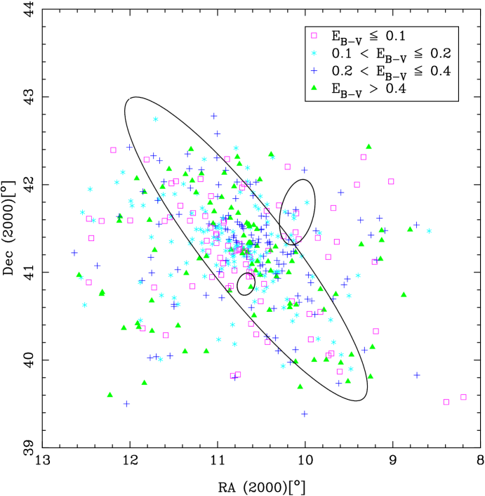
Figure 4: Map of the confirmed and candidate GCs in M31. The large ellipse is the M31 disc/halo boundary as defined by Racine (1991); the two small ellipses are the $D_{25}$ isophotes of NGC 205 (northwest) and M32 (southeast).

Vetešnik (1962b) analysed the photometry of M31 GCs published by Vetešnik (1962a). He assumed that the halo clusters are only affected by foreground Galactic extinction. He derived a mean intrinsic colour of $(B-V)_{0}=0.83$ mag from the objects in the halo of M31 and calculated the colour excess for each object. Subsequently, he studied the reddening distribution of M31 GCs on either side of the major axis and found that the GCs on the northwestern side of the disc are either intrinsically redder, or suffer from more significant extinction, than those on the southeastern side of the disc.

Based on three homogeneous and independent photometric data sets for M31 GC candidates, Iye & Richter (1985) examined the differential reddening towards these objects, and found that the GCs on the northwestern side of the disc are redder than those on the southeastern side. Therefore, Iye & Richter (1985) concluded that the northwestern side of the disc of M31 is nearer to us than its southeastern side.

With the large sample of M31 clusters (and candidates) at hand, we can now also examine the reddening distribution of M31 objects on either side of the major axis, and calculate the mean $E(B-V)$.

Following Perrett et al. (2002) and Huchra et al. (1991), we use the $X,Y$ plane to indicate the position of the GCs. The $X$ coordinate is the position along the major axis of M31, where positive $X$ is in the northeastern direction, while the $Y$ coordinate is along the minor axis of the M31 disc, increasing towards the northwest. The relative coordinates of the M31 clusters are derived by assuming standard geometric parameters for M31. We adopted a central position for M31 at $\rm\alpha_{0}=00^{h}42^{m}44^{s}.30$ and $\rm\delta_{0}=+41^{o}16^{\prime}09^{\prime\prime}.0$ (J2000.0) following Huchra et al. (1991) and Perrett et al. (2002). Formally,

$$X=A\sin\theta+B\cos\theta\quad;$$ (7)

$$Y=-A\cos\theta+B\sin\theta\quad,$$ (8)

where $A=\sin(\alpha-\alpha_{0})\cos\delta$ and $B=\sin\delta\cos\delta_{0}-\cos(\alpha-\alpha_{0})\cos\delta\sin\delta_{0}$. We adopt a position angle of $\theta=38^{\circ}$ for the major axis of M31 (Kent, 1989). Fig. 5 shows graphically the dependence of the average reddening on the distance from the major axis. The error bars represent the standard deviations of the means. It is clear that the reddening on the northwestern (NW) side of the disc is much greater than that on the southeastern (SE) side. The mean reddening on the northwestern and southeastern sides is $\overline{E(B-V)}=0.33\pm 0.02$ and $0.24\pm 0.02$ mag, respectively.

Figure 5: Reddening distribution dependence on the distance from the major axis of M31. The dashed lines indicate the mean reddening values for GCs on the two sides.

Below, we will check our resulting reddening values by studying the distribution of the colours of the M31 clusters and cluster candidates as a function of the projected distance, $Y$, from the major axis. If our reddening values are correct, the distribution of the intrinsic colours of the M31 clusters should be symmetric, even if the distribution of the observed colours is asymmetric. The left-hand panel of Fig. 6 shows the distribution of the mean colours of the GCs and GC candidates binned in 5.5 arcmin intervals in $Y$. The error bars represent the standard deviations of the means. It is clear that the colour distribution is asymmetric. The right-hand panel of Fig. 6 shows the distribution of the mean intrinsic colours of the GCs and GC candidates binned in 5.5 arcmin intervals in $Y$. Again, the error bars represent the standard deviations of the means. Obviously, the distribution of the mean intrinsic colours is nearly symmetric. On the southeastern side, the mean intrinsic colour is $\overline{(B-V)_{0}}$= 0.64$\pm$0.03, while on the northwestern side the mean intrinsic colour is $\overline{(B-V)_{0}}$=0.66$\pm$0.02.

Figure 6: $(B-V)$ colour and intrinsic $(B-V)_{0}$ colour versus distance from the major axis of M31 for M31 GCs and GC candidates.

4 M31 Globular Cluster Metallicities

It is evident that the metallicity distribution of a galaxy’s GC system can provide important clues as to the process and conditions relevant to galaxy formation. Previous studies of the M31 GC system have presented some important information. For example, signs of bimodality were found in the M31 metallicity distribution by Huchra et al. (1991), Ashman & Bird (1993), Barmby et al. (2000) and Perrett et al. (2002). In addition, Huchra et al. (1991) found that the metal-rich clusters in M31 appear to form a central rotating disc system. Based on the current largest sample including 321 velocities, Perrett et al. (2002) performed a more comprehensive investigation into the kinematics of the M31 cluster system and showed that the metal-rich GCs appear to constitute a distinct kinematic subsystem that demonstrates a centrally concentrated spatial distribution with a high rotation amplitude, but it does not appear to be significantly flattened. This is consistent with a bulge population. In this section, we will examine the distribution of GC metallicities in M31 using the largest number of GCs and GC candidates available to date. We will include the metallicities determined based on GC colours.

4.1 Colour-derived metallicities

In total, 231 of the GCs and GC candidates in our sample of 443 objects with reliable reddening values have no spectroscopic metallicities. Therefore, we will determine their metallicities based on the C-M relation for these objects. From the colour excesses of GCs with spectroscopic metallicities, Barmby et al. (2000) found that the M31 and Galactic GC C-M relations are consistent. Therefore, in this section, we will determine metallicities for 231 GCs and GC candidates from their intrinsic colours by applying the Galactic C-M relation. We use bi-sector linear fits (Akritas & Bershady, 1996) to determine the metallicity as a function of colour, and average the resulting metallicities over the available colours for each object (except for some significantly deviating points that are most likely due to inaccurate photometric data, i.e. those that differ from the mean value by more than $1\sigma$, as justified above). As in the reddening determination, the standard deviations of the metallicities from individual colours are used as the error estimates. There are 209 GCs (and candidates) with metallicity determinations, which are listed in Table 5.

4.2 Comparison of spectroscopic and colour-derived metallicities

In this section, we will test the process outlined in Section 4.1 by applying it to the clusters with spectroscopic metallicities; this includes all GCs for which the metallicities can be determined based on the C-M relation fits. The results of our comparison are shown in Fig. 7; the mean metallicity offset (spectroscopic minus colour-derived metallicity) is $0.039\pm 0.022$ dex. From Fig. 7 we can see that there is no evidence of a bias in the prediction of the metallicities. The offsets for all clusters are less than 0.7 dex, and the offsets for 4 clusters are greater than 0.5 dex. Since some of these metallicity differences are substantial, we have carefully double checked our data and results. In fact, the large spread in metallicity space is also evident from fig. 10 of Barmby et al. (2000). However, upon close examination of the data, we found that there are 4 objects that should not be included in the calculation of the offset between spectroscopic and colour-derived metallicities, i.e. objects B068, B075, B159 and B219. For B068, we determined 14 colour-derived metallicities, and these colour-derived metallicities have a small scatter. Their mean value is ${\rm[Fe/H]=-0.81\pm 0.03}$ dex. However, the spectral metallicity is ${\rm[Fe/H]=-0.29\pm 0.59}$ dex; we suspect that the spectral metallicity determination may be incorrect. For B075, there are only three colour-derived metallicities, the mean value of which is ${\rm[Fe/H]=-1.71\pm 0.08}$ dex. On the other hand, the spectral metallicity is ${\rm[Fe/H]=-1.03\pm 0.33}$ dex, so that we think that more photometric data is needed to determine the colour-derived metallicities more accurately. For B159, there are also only three colour-derived metallicities. Their mean value is ${\rm[Fe/H]=-2.33\pm 0.11}$ dex, whilst the GC’sspectral metallicity is ${\rm[Fe/H]=-1.58\pm 0.41}$ dex. Therefore, we also think that more photometric data is needed to determine its colour-derived metallicity more accurately. Finally, for B219 we determined 14 colour-derived metallicities, which exhibit a small scatter. The mean value of these metallicities is ${\rm[Fe/H]=-0.62\pm 0.05}$ dex. However, the spectral metallicity is ${\rm[Fe/H]=-0.01\pm 0.57}$ dex, while we also suspect that this spectral metallicity may be problematic. Except for these four clusters, the mean metallicity offset (spectroscopic minus colour-derived metallicity) is $0.028\pm 0.022$ dex, compared with $0.020\pm 0.021$ found by Barmby et al. (2000) based on a smaller GC sample. This bias in the metallicity determination may come from large errors in either the colour- or spectroscopically determined metallicities, or both. In addition, the correlations between optical colours and metallicity, which are used to determine the colour-derived metallicity for M31 clusters, are constructed based on the Galactic GCs, which may have introduced a small (but likely insignificant) bias. In the following analysis, we have substracted this offset from all of our colour-derived metallicities. Fig. 8 shows the metallicity distributions of the spectroscopic and colour-derived samples (cf. Fig. 7). Here, we now use a Kolmogorov-Smirnov (KS) test to demonstrate whether the two distributions in Fig. 8 are the same. We determined a value of $D_{\rm max}=0.061$ for these two samples (which do not include the four objects noted above); $D_{\rm max}$ is defined as the maximum value of the absolute difference between two cumulative distribution functions. The probability of obtaining a value of $D_{\rm max}=0.061$ is 80.8%. It is clear that the KS test supports the similarity of the metallicity distributions of the spectroscopic and colour-derived samples.

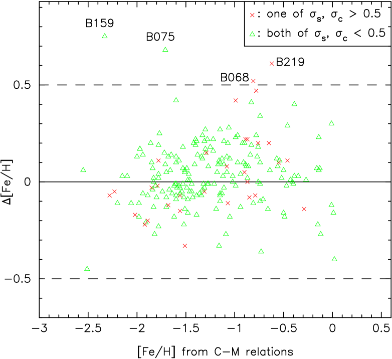
Figure 7: Comparison of spectroscopic and colour-derived metallicities for M31 GCs with spectroscopic data; $\sigma_{\rm s}$ indicates the uncertainty in the spectroscopic metallicity and $\sigma_{\rm c}$ is based on the C-M relations.

Figure 8: Comparison of spectroscopic and colour-derived metallicity distributions.

Table 5: New metallicity estimates for M31 GCs and GC candidates without spectroscopic observations.

Name	$\rm[Fe/H]$	Name	$\rm[Fe/H]$	Name	$\rm[Fe/H]$	Name	$\rm[Fe/H]$	Name	$\rm[Fe/H]$
B290	$-1.07\pm 0.07$	BA21	$-2.51\pm 0.11$	B412	$-0.80\pm 0.02$	B413	$-1.57\pm 0.08$	B134D	$-2.41\pm 0.23$
B291	$-1.12\pm 0.04$	B138D	$-0.36\pm 0.04$	B140D	$-1.57\pm 0.12$	B141D	$-1.07\pm 0.08$	B142D	$-2.59\pm 0.24$
B144D	$-1.62\pm 0.09$	B148D	$-1.93\pm 0.21$	B149D	$-2.21\pm 0.25$	B150D	$-2.52\pm 0.07$	B416	$-1.34\pm 0.07$
B152D	$-2.55\pm 0.09$	B418	$-1.19\pm 0.10$	B154D	$-0.53\pm 0.83$	B156D	$-2.58\pm 0.14$	B420	$-0.63\pm 0.07$
B157D	$-0.09\pm 0.08$	B422	$-1.97\pm 0.18$	B162D	$-2.53\pm 0.17$	B163D	$0.20\pm 0.06$	B424	$-2.09\pm 0.10$
B165D	$-1.05\pm 0.13$	B166D	$-1.02\pm 0.08$	B167D	$-2.34\pm 0.08$	B427	$-1.57\pm 0.08$	B169D	$-0.10\pm 0.04$
B428	$-2.04\pm 0.09$	B172D	$-2.51\pm 0.12$	B175D	$0.31\pm 0.09$	B177D	$-1.32\pm 0.01$	B433	$-2.45\pm 0.14$
B435	$-1.76\pm 0.12$	B178D	$-0.90\pm 0.24$	B309	$-2.03\pm 0.26$	B181D	$-2.21\pm 0.20$	B438	$-2.42\pm 0.31$
B186D	$-2.08\pm 0.14$	B440	$-0.41\pm 0.09$	B003	$-2.08\pm 0.07$	B188D	$-1.84\pm 0.14$	B325	$-1.77\pm 0.08$
B192D	$-0.46\pm 0.03$	B330	$-1.98\pm 0.06$	B004D	$-1.17\pm 0.05$	B194D	$-1.97\pm 0.12$	B447	$-1.73\pm 0.12$
B244	$-1.50\pm 0.21$	B014	$-0.55\pm 0.13$	B197D	$-0.69\pm 0.05$	B450	$-0.89\pm 0.05$	B022	$-1.64\pm 0.07$
B339	$-0.90\pm 0.04$	B202D	$-0.74\pm 0.04$	B020D	$-0.76\pm 0.08$	B032	$-1.09\pm 0.03$	B456	$-1.71\pm 0.29$
B203D	$-2.03\pm 0.08$	B457	$-1.60\pm 0.21$	B204D	$-1.18\pm 0.10$	B025D	$-1.28\pm 0.10$	B205D	$-2.35\pm 0.21$
B207D	$-0.27\pm 0.08$	B052	$0.12\pm 0.17$	B060	$-1.87\pm 0.06$	B062	$-0.47\pm 0.11$	B067	$-2.55\pm 0.04$
B257	$-2.05\pm 0.82$	B461	$-2.56\pm 0.07$	B070	$-1.66\pm 0.10$	B078	$-0.56\pm 0.15$	B079	$-0.85\pm 0.03$
B345	$-1.40\pm 0.06$	B462	$-2.28\pm 0.34$	B084	$-0.76\pm 0.07$	B346	$-1.70\pm 0.07$	B347	$-1.71\pm 0.03$
B348	$-1.38\pm 0.07$	B463	$-1.46\pm 0.18$	B099	$-1.03\pm 0.06$	B100	$-2.21\pm 0.10$	B101	$-1.17\pm 0.02$
NB46	$-1.48\pm 0.03$	NB70	$-2.48\pm 0.04$	B464	$-0.44\pm 0.09$	B111	$-1.50\pm 0.03$	B260	$-0.36\pm 0.10$
NB64	$-2.12\pm 0.46$	B118	$-1.64\pm 0.10$	B351	$-1.60\pm 0.05$	NB25	$-0.31\pm 0.08$	B123	$-1.58\pm 0.04$
B128	$-0.92\pm 0.05$	NB50	$-2.23\pm 0.19$	B136	$-2.39\pm 0.08$	B217D	$-2.36\pm 0.04$	B266	$-2.80\pm 0.15$
B220D	$-2.69\pm 0.13$	B221D	$-1.56\pm 0.15$	B150	$-0.76\pm 0.08$	B223D	$-0.23\pm 0.08$	B468	$-2.16\pm 0.12$
B155	$-0.84\pm 0.03$	B226D	$-2.01\pm 0.19$	B162	$-0.70\pm 0.05$	B228D	$0.27\pm 0.14$	B168	$-0.12\pm 0.21$
B169	$-2.56\pm 0.06$	B172	$-0.87\pm 0.03$	DAO062	$-2.13\pm 0.14$	B173	$-1.86\pm 0.47$	B177	$-0.88\pm 0.10$
B181	$-1.10\pm 0.03$	B231D	$-0.12\pm 0.07$	B470	$-2.18\pm 0.23$	B187	$-1.72\pm 0.04$	B471	$-2.18\pm 0.09$
B189	$0.18\pm 0.11$	B194	$-1.56\pm 0.05$	B195	$-1.48\pm 0.63$	B196	$-1.94\pm 0.08$	B202	$-1.84\pm 0.11$
B361	$-1.61\pm 0.02$	B237D	$-0.78\pm 0.26$	G260	$-2.45\pm 0.06$	B239D	$-1.67\pm 0.13$	B215	$-1.21\pm 0.03$
G268	$-1.36\pm 0.01$	B243D	$-1.28\pm 0.07$	B245D	$-2.88\pm 0.09$	B473	$-2.17\pm 0.16$	B247D	$-1.90\pm 0.23$
B227	$-1.28\pm 0.08$	B250D	$-0.98\pm 0.14$	B252D	$-2.83\pm 0.09$	B474	$-2.12\pm 0.10$	B256D	$-2.37\pm 0.13$
B476	$-0.03\pm 0.13$	B236	$-1.01\pm 0.17$	B258D	$-2.47\pm 0.08$	B260D	$-1.46\pm 0.15$	B478	$-2.69\pm 0.01$
B261D	$-2.45\pm 0.19$	B263D	$-0.85\pm 0.07$	B286	$-1.67\pm 0.11$	B479	$-0.36\pm 0.13$	B266D	$-2.34\pm 0.10$
B481	$-1.45\pm 0.13$	B270D	$-2.28\pm 0.19$	B273D	$-1.01\pm 0.03$	B274D	$-0.08\pm 0.11$	B275D	$-1.81\pm 0.13$
B277D	$-0.83\pm 0.06$	B278D	$-2.46\pm 0.19$	B385	$-0.86\pm 0.14$	B283D	$-1.55\pm 0.17$	B288D	$-2.58\pm 0.23$
B489	$-0.04\pm 0.10$	B490	$0.08\pm 0.07$	G325	$0.12\pm 0.12$	B389	$-0.35\pm 0.08$	B293D	$-2.57\pm 0.11$
B295D	$-2.22\pm 0.13$	B296D	$-0.91\pm 0.16$	B297D	$0.10\pm 0.08$	B298D	$-2.35\pm 0.11$	B299D	$-1.91\pm 0.10$
B300D	$-2.52\pm 0.11$	B393	$-1.41\pm 0.05$	B492	$-1.06\pm 0.27$	B302D	$-1.30\pm 0.05$	B304D	$-2.41\pm 0.12$
B493	$1.07\pm 0.28$	B494	$-1.54\pm 0.05$	B307D	$-1.64\pm 0.10$	B308D	$-2.43\pm 0.14$	B495	$-0.35\pm 0.05$
B396	$-1.87\pm 0.09$	B310D	$-0.93\pm 0.05$	B313D	$-1.00\pm 0.16$	B314D	$-0.18\pm 0.06$	B317D	$-2.47\pm 0.13$
B319D	$-1.86\pm 0.17$	B320D	$-2.62\pm 0.15$	B324D	$-2.27\pm 0.00$	B398	$-0.72\pm 0.08$	B399	$-1.69\pm 0.09$
B326D	$-0.63\pm 0.08$	B328D	$-1.67\pm 0.06$	B329D	$-0.24\pm 0.04$	B330D	$-0.55\pm 0.06$	B331D	$-1.50\pm 0.08$
B332D	$-0.65\pm 0.09$	B402	$-1.18\pm 0.06$	B334D	$-0.75\pm 0.06$	B338D	$-1.86\pm 0.06$	B339D	$-1.51\pm 0.04$
B340D	$0.19\pm 0.29$	B508	$-2.61\pm 0.07$	B343D	$-0.49\pm 0.05$	B344D	$-1.40\pm 0.03$	B345D	$-0.39\pm 0.12$
B346D	$-0.37\pm 0.19$	B347D	$0.00\pm 0.15$	B348D	$-1.16\pm 0.26$	B349D	$-0.76\pm 0.26$

4.3 Metallicity distribution

The metallicity distribution of the M31 clusters has been investigated in previous studies, including Huchra et al. (1991), Ashman & Bird (1993), Barmby et al. (2000) and Perrett et al. (2002). With the current largest GC and GC candidate sample at hand, we will now reanalyse the M31 GC metallicity distribution. Including the metallicities determined based on the C-M fits, our sample includes a total of 504 metallicities.

Fig. 9 shows the metallicity distribution of the M31 GCs discussed in this paper, along with a similar figure for the Milky Way GCs (from H03), for comparison. To assess whether the combination of spectral and colour-derived metallicities has an effect on the results, we consider three data sets in our analysis of the metallicity distribution of the M31 objects: Set 1 contains all objects for which metallicities have been determined from spectroscopic observations; Set 2 contains the metallicities without spectroscopic observations, which have been determined based on the C-M relationships in this paper; and Set 3 contains all metallicities from Sets 1 and 2. The mean metallicities of Sets 1, 2, and 3 are [Fe/H] = $-1.202\pm 0.036$, $-1.414\pm 0.057$, and $-1.290\pm 0.032$ dex, respectively, i.e. comparable to (although not in all cases the same as) the value of $\rm[Fe/H]=-1.21\pm 0.03$ dex obtained by Perrett et al. (2002), and also comparable to the value of $\rm[Fe/H]=-1.298\pm 0.046$ dex obtained for the Milky Way GCs (H03). However, we point out that the mean metallicities of Sets 1 and 2 are different at the $3\sigma$ level. We investigated this result carefully, and found that there are many more objects of which the metallicities determined based on the C-M relationships in this paper are lower than $\rm[Fe/H]=-2.5$, compared to the number of GCs for which metallicities were determined from spectroscopic observations. Generally speaking, the objects without spectroscopic observations are fainter than those with spectroscopic observations. Therefore, we should keep in mind that the objects for which the metallicities have been determined based on the C-M relationships are fainter than those with spectroscopic observations. The photometry is more accurate for bright than for faint objects, however. For bright clusters, i.e., those with spectroscopic observations, the metallicities determined based on the C-M relationships are consistent with those determined from spectroscopic observations (see Fig. 8). In fact, Barmby et al. (2000) did not use the very high or low metallicity values, $\rm[Fe/H]>0.5$ or $\rm[Fe/H]<-2.5$ dex, obtained based on the C-M relationships in their paper when investigating the metallicity distribution. If we exclude these very high or low metallicity values, the mean metallicities of Sets 1 and 2 are the same. At the same time, we emphasize that there are no reasons for not using these low or high metallicities when investigating the metallicity distribution for M31 GCs. The asymmetric appearance of the metallicity distribution in Fig. 9 suggests the possibility of bimodality. We use the KMM algorithm (McLachlan & Basford, 1988; Ashman et al., 1994) to search for bimodality in the metallicity distribution. The input of the KMM algorithm includes the individual data points, the Gaussian group membership to be fitted, and starting values for the estimated means and common variance. In fact, for two-group homescedastic fitting, the KMM algorithm is insensitive to these input values and converges to the “correct” two-group fit even when its starting points are far from the true means and variance (see details in Ashman et al., 1994). We assumed the same variances for both groups in the metallicity distribution; in this homoscedastic fitting the $p$-value of the hypothesis test returned by the KMM algorithm adequately indicates that a two-group fit is an improvement with respect to a one-group fit. Table 6 lists the parameters returned by the KMM algorithm. It is clear that the metallicity distributions of both data sets show strong bimodality. Thus, the KMM tests suggest that we can consider these two distributions of metallicity bimodal at the $\sim 100$ per cent confidence level. We also investigated the KMM results based on three groups and on heteroscedastic two-group fits. The results of these exercises are listed in Tables 7 and 8, which show that three-group and heteroscedastic two-group fits are also statistically acceptable. We point out that KMM tests assume Gaussian distributions, which may or may not be realistic here. In the following analysis, we investigate the metallicity distribution for all samples in this paper, for which the homescedastic two-group fits may be more appropriate (see Tables 6, 7 and 8). We also apply the Dip test to confirm whether or not the metallicity distributions of our M31 GC samples are multimodal. The Dip statistic is the maximum difference between the empirical distribution function, and the unimodal distribution function that minimizes the maximum difference (see details in Hartigan & Hartigan, 1985; Hartigan, 1985). The Dip statistic measures the departure of the sample’s unimodality. If its value approaches zero, the samples are taken from a unimodal distribution; if the Dip measure is positive, the samples come from a multimodal distribution. The Dip values for Sets 1, 2 and 3 are 0.024, 0.025 and 0.018 with significance values of 71.2%, 55.43% and 66.9%, respectively, which shows that the Dip values support the multimodality found from the KMM tests. We note that the Dip value for the (bimodal) metallicity distribution of the Galactic GCs is 0.039 with significance value of 90.5%.

Figure 9: Metallicity distributions and homescedastic bimodal KMM tests of M31 GCs and GC candidates, subdivided by uncertainty, and Galactic GCs.

Table 6: Results from the KMM homescedastic bimodality tests for the metallicities of the GCs in M31 and the Milky Way.

Data Set	$\overline{\rm[Fe/H]}$	$\sigma_{\rm[Fe/H]}$	$\overline{\rm[Fe/H]_{1}}$	$\overline{\rm[Fe/H]_{2}}$	$\sigma_{\rm[Fe/H]}$	$n_{1}$	$n_{2}$	$p$
1	$-1.202\pm 0.036$	0.617	$-1.558$	$-0.676$	0.438	182	113	0.032
2	$-1.414\pm 0.057$	0.828	$-1.948$	$-0.619$	0.508	124	85	0.000
3	$-1.290\pm 0.032$	0.719	$-1.740$	$-0.722$	0.510	284	220	0.004
MW	$-1.298\pm 0.046$	0.564	$-1.620$	$-0.608$	0.306	101	47	0.000

Table 7: Results from the KMM heteroscedastic bimodality tests for the metallicities of the GCs in M31.

Data Set	$\overline{\rm[Fe/H]_{1}}$	$\overline{\rm[Fe/H]_{2}}$	$\sigma_{1,\rm[Fe/H]}$	$\sigma_{2,\rm[Fe/H]}$	$n_{1}$	$n_{2}$	$p$
1	$-1.487$	$-0.574$	0.466	0.401	207	88	0.145
2	$-2.424$	$-1.192$	0.180	0.743	44	165	0.000
3	$-1.794$	$-0.786$	0.488	0.534	254	250	0.022

Table 8: Results from the KMM homescedastic trimodality tests for the metallicities of the GCs in M31.

Data Set	$\overline{\rm[Fe/H]_{1}}$	$\overline{\rm[Fe/H]_{2}}$	$\overline{\rm[Fe/H]_{3}}$	$\sigma_{\rm[Fe/H]}$	$n_{1}$	$n_{2}$	$n_{3}$	$p$
1	$-1.733$	$-1.100$	$-0.462$	0.374	120	114	61	0.128
2	$-2.141$	$-1.159$	$-0.266$	0.399	92	78	39	0.000
3	$-1.985$	$-1.206$	$-0.434$	0.419	162	237	105	0.012

4.4 Spatial distribution

In the previous section, we investigated the metallicity distribution of the M31 GCs based on the KMM test. The KMM test allows us to distinguish between the metal-poor and metal-rich subsamples, i.e., the KMM test gives [Fe/H]=-1.18 dex as the dividing line between the metal-poor and metal-rich GCs. However, there are about 54 objects that exhibit intermediate probabilities of membership in both groups ($0.5<prob.<0.6$). Since it is difficult to decide unequivocally which group these objects belong to, we simply adopted the dividing line between metal-poor and metal-rich GCs from the KMM test.

Figure 10 shows the projected spatial distributions of the metal-poor and metal-rich GCs in M31. Using Eqs. (7) and (8), we obtained the distances to our sample clusters from the centre of M31. From Fig. 10, it is clear that the metal-rich GCs in M31 are more centrally concentrated, consistent with what was found by Huchra et al. (1991) and Perrett et al. (2002). The metal-poor GCs appear to occupy a more extended halo, although also with a general concentration following the outline of the M31 disc. The latter may have been caused by selection biases, i.e., from Fig. 4 we can see that there are more clusters observed along the major axis than the minor axis. Fig. 11 shows the histograms of the metal-poor and metal-rich populations. A notable shortage of metal-poor clusters in the innermost radial bins can clearly be seen, which is also consistent with the results of Perrett et al. (2002). In the Milky Way, the metal-rich GCs reveal significant rotation and have historically been associated with the thick-disc system (Zinn, 1985; Armandroff, 1989); however, other studies (Frenk & White, 1982; Minniti, 1995; $\rm{C\hat{o}t\acute{e}}$, 1999; Forbes et al., 2001) have suggested that metal-rich GCs within $\sim 5$ kpc of the Galactic Centre are more appropriately associated with the Milky Way’s bulge and/or bar. In M31, Elson & Walterbos (1988) showed that the metal-rich clusters constitute a more highly flattened system than the metal-poor ones, and appear to have disc-like kinematics; Huchra et al. (1991) showed that the metal-rich GCs are preferentially located close to the galactic centre. Huchra et al. (1991) also showed that the distinction between the rotation of the metal-rich and metal-poor clusters is most apparent in the inner 2 kpc. Therefore, they concluded that the metal-rich clusters in M31 appear to form a central rotating disc system. Perrett et al. (2002) performed a more comprehensive investigation into the kinematics of the M31 cluster system. They showed that the metal-rich M31 GCs appear to constitute a distinct kinematic subsystem that demonstrates a centrally concentrated spatial distribution with a high rotation amplitude, but that does not appear significantly flattened, consistent with a bulge population. Schroder et al. (2002) performed a maximum-likelihood kinematic analysis of 166 M31 clusters taken from Barmby et al. (2000) and found that the most significant difference between the rotation of the metal-rich and metal-poor clusters occurs at intermediate projected galactocentric radii. Particularly, Schroder et al. (2002) presented a potential thick-disc population among M31’s metal-rich GCs.

Figure 10: Spatial distribution of the metal-rich and metal-poor GCs in M31.

Figure 11: Radial distribution of the metal-rich and metal-poor GCs and GC candidates in M31.

4.5 Metallicity gradient

The presence or absence of a radial trend in the metallicity of a GC sample is an important test of galaxy formation theories (Barmby et al., 2000). In the Eggen et al. (1962) galaxy formation scenario, the halo stars and GCs should show large-scale metallicity gradients (Eggen et al., 1962; Barmby et al., 2000); however, in the Searle & Zinn (1978) scenario the expected metallicity distribution is more homogeneous. For the Milky Way, Armandroff (1989) provided some evidence that metallicity gradients with both distance from the Galactic plane and distance from the Galactic Centre are present in the disc cluster system. For M31, there are some inconsistent conclusions, e.g., van den Bergh (1969) showed that there is little or no evidence for a correlation between metallicity and projected radius, but most of his clusters were located inside a radius of 50 arcmin; however, some authors (see, e.g., Huchra et al., 1982; Sharov, 1988; Huchra et al., 1991; Perrett et al., 2002) showed that there is evidence for a weak but measurable metallicity gradient as a function of projected radius. Barmby et al. (2000) confirmed the latter result based on their large sample of spectral and colour-derived metallicities.

In Fig. 12, we show the metallicity of the M31 GCs as a function of galactocentric radius based on our large cluster sample. It is clear that the dominant feature of this diagram is the scatter in metallicity at any radius. However, it is also true that a trend of decreasing metallicity with increasing galactocentric distance exists, for both the metal-poor and the entire population. The slopes of the metal-poor subsample and for the entire sample are $-0.006\pm 0.001$ and $-0.007\pm 0.002$ dex arcmin^-1, respectively, while for metal-rich sample, it is $0.000\pm 0.001$ dex arcmin^-1. The latter can certainly be considered as no metallicity gradient. In order to show this, we display the mean metallicity binned in 10 arcmin intervals in galactocentric radius. We can see that, within $\sim 90$ arcmin, the mean metallicity decreases with galactocentric radius for both the metal-poor and for the entire population. The error bars represent the standard deviations of the means. These results are in good agreement with Perrett et al. (2002) and Huchra et al. (1991). Therefore, we can conclude that simple smooth, pressure-supported collapse models of galaxies by themselves are unlikely to fit M31.

Figure 12: Metallicity distribution versus projected radius for the entire and the metal-poor populations of the M31 GCs and GC candidates.

4.6 Metallicity versus intrinsic magnitude

The (possible) correlation between cluster mass (or luminosity) and metallicity is important in GC formation theory. It is generally believed that if self-enrichment is important in GCs, the most massive clusters could retain their metal-enriched supernova ejecta, so that the metal abundance should increase with cluster mass; the opposite is true if cooling from metals determines the temperature in the cluster-forming clouds (Barmby et al., 2000). The possible self-enrichment of GCs has been studied in detail in some aspects (see details in Strader et al., 2006). However, the model of GC self-enrichment developed by Parmentier et al. (1999) is particularly interesting in this context. In this model, cold and dense clouds embedded in the hot proto-galactic medium are assumed to be the progenitors of galactic halo GCs. Based on this model, Parmentier & Gilmore (2001) suggested that the most metal-rich proto-GCs are the least massive ones.

The HST provides a unique tool to study GCs in external galaxies. Recently, using the ACS onboard the HST, Harris et al. (2006), Mieske et al. (2006) and Strader et al. (2006) found that in giant ellipticals – such as M87, NGC 4649 and NGC 7094 (although not in NGC 4472) – luminous blue GCs reveal a trend of having redder colours, such that more massive GCs are redder (more metal-rich). This trend is referred to as the “blue tilt” (see also Brodie & Strader, 2006). This blue tilt has been interpreted as a result of self-enrichment (Strader et al., 2006). Strader et al. (2006) speculatively suggested that these GCs once possessed dark matter haloes. Spitler et al. (2006) subsequently found that this blue tilt is also present in the Sombrero spiral galaxy (NGC 4594) and may extend to less luminous GCs with a somewhat shallower slope than derived by Harris et al. (2006) and Strader et al. (2006). As Spitler et al. (2006) pointed out, the Sombrero galaxy provides the first example of this trend in a spiral galaxy, and in a galaxy found in a low-density galaxy environment. However, in these ACS studies, the metal-rich (redder) GCs did not show a corresponding trend (see also Bekki et al., 2007). Based on high-resolution cosmological simulations including GCs, Bekki et al. (2007) investigated the formation processes and physical properties of GC systems in galaxies, and found that luminous metal-poor clusters would develop a correlation between luminosity and metallicity if they originated from the nuclei of low-mass galaxies at high redshift. In fact, in the simulations of Bekki et al. (2007), the “simulated blue tilts” come from the assumption that luminous metal-poor clusters originate from the stellar galactic nuclei of the more massive nucleated galaxies exhibiting a luminosity-metallicity relation. It is therefore evident that, in Bekki et al. (2007), galaxies which experienced more accretion/merging events of nucleated low-mass galaxies are more likely to show a blue tilt.

Fig. 13 shows the diagram of GC metallicity versus dereddened apparent magnitude. It is clear that there is no obvious trend of metallicity with luminosity similar to that in Huchra et al. (1991) and Barmby et al. (2000). Least-squares fits show no evidence for a relationship between luminosity and metallicity in our sample clusters.

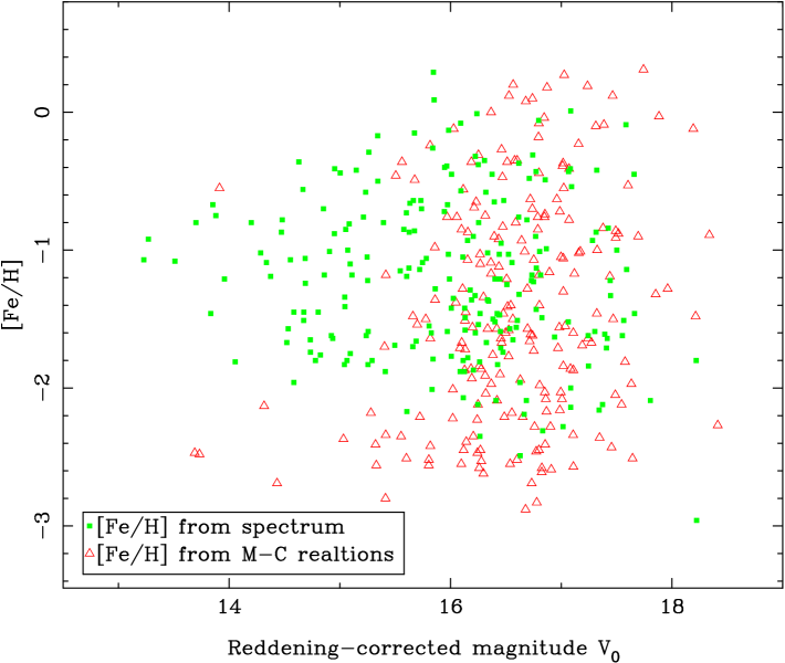
Figure 13: Metallicity as a function of the reddening-corrected magnitude $V_{0}$ for our sample GCs.

5 Discussion and Conclusions

In this paper, we have (re-)determined the reddening values for 443 clusters and cluster candidates in M31, as well as metallicities for 209 sample objects without spectroscopic observations. We have followed the methods described by Barmby et al. (2000), who found that the M31 and Galactic extinction laws are the same within the observational errors, and that the M31 and Galactic GC C-M relations are also consistent with each other. The sample of spectroscopic and photometric data used in this paper is the newest and largest to date. The spectroscopic data were obtained from the most recent references currently available and the photometric data are from the most comprehensive catalogue of M31 clusters available at present, which includes 337 confirmed GCs and 688 GC candidates. Using the metallicities of the largest sample of clusters and cluster candidates at hand, we studied the properties of the M31 clusters. Our main conclusions are summarised below:

1. The reddening distribution shows that slightly more than 50 per cent of the GCs suffer from a reddening of less than $E(B-V)=0.2$ mag, and the mean value is $E(B-V)=0.28_{-0.14}^{+0.23}$ mag. The spatial distribution of $E(B-V)$ indicates that the reddening on the northwestern side of the M31 disc is greater than that on the southeastern side, which is consistent with the conclusion that the northwestern side in nearer to us.

2. The metallicity distribution of the M31 GCs is bimodal with peaks at $\rm{[Fe/H]}\approx-1.7$ and $-0.7$ dex.

3. The diagram of metallicities as a function of radius from the M31 centre shows a metallicity gradient for the metal-poor GCs, but no such gradient for the metal-rich GCs.

4. The metal-rich clusters appear to constitute a centrally concentrated spatial distribution; however, the metal-poor clusters tend to be less spatially concentrated.

5. There is no correlation between luminosity and metallicity among our M31 sample clusters, which indicates that self-enrichment is indeed unimportant for cluster formation in M31.

We reiterate that in using the method of Barmby et al. (2000), there are two major unavoidable assumptions (acknowledged by these authors), i.e. that in the Milky Way and in M31 both the extinction law and the intrinsic colours of the GCs are the same. The latter assumption seems reasonable, since there is no evidence that GCs in different galaxies have different intrinsic colours. Regarding the former assumption, there is inconsistent evidence as to whether or not this is a valid assumption. For example, Walterbos & Kennicutt (1988) found that the extinction law in M31 is very similar to that in the Milky Way, by analysing the two major dust lanes on the near side of M31; however, several studies have suggested that the reddening in M31 appears to be peculiar: with $E(U-B)/E(B-V)=1.01\pm 0.11$ (Iye & Richter, 1985) and $E(U-B)/E(B-V)\sim 0.5$ (Massey et al., 1995), compared to 0.72 for the same ratio in the Milky Way. Based on a large sample of GCs with optical and near-infrared photometric data, Barmby et al. (2000) demonstrated that the $U$- and $K$-band extinction curve of M31 is consistent with that of the Milky Way, with total-to-selective extinction coefficient $R_{V}=3.1$. In fact, the former assumption is plausible because in the M31 disc the composition and size distribution of the large normal grains which dominate the dust mass may be similar to those in the Milky Way (see for details, Xu & Helou, 1996).

As an example, we will discuss in some detail the reddening value of the M31 GC B037 (a.k.a. 037-B327), which is known to be an extremely red object. There are a few references that discuss this GC, including Barmby et al. (2002b), Ma et al. (2006a), Ma et al. (2006c) and Cohen (2006). Kron & Mayall (1960) first noticed an extremely red colour in photographic ($P$) and visual ($V$) bands for B037, and determined its absorption to be $A_{V}=3.90$ mag. Based on the photometric data for M31 star clusters in $U,B$, and $V$ of Vetešnik (1962a), Vetešnik (1962b) studied the reddening values for these objects and found that B037 was the most highly reddened in his sample, with $E(B-V)=1.28$ mag ($A_{V}=4.10$ mag). Crampton et al. (1985) calibrated $(B-V)_{\rm 0}$ as a function of spectroscopic slope parameter $S$ of the continuum between $\sim 4000$ and 5000 Å, and then determined the intrinsic colours for about 40 GCs and GC candidates, including B037. Crampton et al. (1985) presented a reddening value for B037 of $E(B-V)=1.48$ mag. Armed with a large database of multicolour photometry, Barmby et al. (2000) determined the reddening value for each individual M31 GC, including B037, using the correlations between optical and infrared colours and metallicity based on various “reddening-free” parameters, and derived $E(B-V)=1.38\pm 0.02$ mag for B037. Using spectroscopic metallicities to predict the intrinsic colours, Barmby et al. (2002b) rederived the reddening value for this GC, $E(B-V)=1.30\pm 0.04$ mag. Recently, Ma et al. (2006a) determined the reddening and age of the B037 by comparing multicolour photometry with theoretical stellar population synthesis models. The reddening towards B037 determined by Ma et al. (2006a) is $E(B-V)=1.360\pm 0.013$ mag. The reddening value for B037 determined in this paper is $E(B-V)=1.21\pm 0.03$ mag. It is clear that the consistent reddening values for B037 from different references confirm that this cluster suffers from very large extinction. In fact, Ma et al. (2006c) showed the dust lane across the face of the cluster using an HST/ACS image, which may partially account for its very large reddening value (see also Cohen, 2006).

References

- Akritas & Bershady (1996) Akritas M. G., Bershady M. A., 1996, ApJ, 470, 706
- Armandroff (1989) Armandroff T. E., 1989, AJ, 97, 375
- Ashman & Bird (1993) Ashman K. M., Bird C. M., 1993, AJ, 106, 2281.
- Ashman et al. (1994) Ashman K. M., Bird C. M., Zepf S. E., 1994, AJ, 108, 2348
- Bajaja & Gergely (1977) Bajaja E., Gergely T. E., 1977, A&A, 61, 229
- Barmby et al. (2000) Barmby P., Huchra J., Brodie J., Forbes D., Schroder L., Grillmair C., 2000, AJ, 119, 727
- Barmby et al. (2002a) Barmby P., Holland S., Huchra J. P., 2002a, AJ, 123, 1937
- Barmby et al. (2002b) Barmby P., Perrett K. M., Bridges T. J., 2002b, MNRAS, 329, 461
- Baum et al. (1995) Baum W. A., et al., 1995, AJ, 110, 2537
- Beasley et al. (2004) Beasley M., et al., 2004, AJ, 128, 1623
- Bekki et al. (2007) Bekki K., Yahagi H., Forbes D. A., 2007, MNRAS, 377, 215
- Bònoli et al. (1987) Bònoli F., Delpino F., Federici L., Fusi Pecci F., 1987, A&A, 185, 25
- Brodie & Huchra (1990) Brodie J. P., Huchra J. P., 1990, ApJ, 362, 503
- Brodie & Strader (2006) Brodie J., Strader J., 2006, ARA&A, 44, 193
- Burstein & Heiles (1982) Burstein D., Heiles C., 1982, AJ, 87, 1165
- Cardelli et al. (1989) Cardelli J. A., Clayton G. C., Mathis J. S., 1989, ApJ, 345, 245
- (1999) P., 1999, AJ, 118, 406
- Cohen (2006) Cohen J. G., 2006, ApJ, 653, L21
- Crampton et al. (1985) Crampton D., Cowley A. P., Schade D., Chayer P., 1985, ApJ, 288, 494
- Djorgovski et al. (1997) Djorgovski S. G., Gal R. R., McCarthy J. K., Cohen J. G., de Carvalho R. R., Meylan G., Bendinelli O., Parmeggiani G., 1997, ApJ, 474, L19
- Eggen et al. (1962) Eggen O. J., Lynden-Bell D., Sandage A. R., 1962, ApJ, 136, 748
- Elias et al. (1982) Elias J. H., Frogel J. A., Matthews K., Neugebauer G., 1982, AJ, 87, 1029
- Elias et al. (1983) Elias J. H., Frogel J. A., Hyland A. R., Jones T. J., 1983, AJ, 88, 1027
- Elson & Walterbos (1988) Elson R. A., Walterbos R. A. M., 1988, ApJ, 333, 594
- Fan et al. (2006) Fan Z., Ma J., de Grijs R., Yang Y., Zhou X., 2006, MNRAS, 371, 1648
- Forbes et al. (2001) Forbes D. A., Brodie J. P., Larsen S. S., 2001, ApJ, 556, L83
- Frenk & White (1982) Frenk C. S., White S. D. M., 1982, MNRAS, 198, 173
- Frogel et al. (1980) Frogel J. A., Persson S. E., Cohen J. G., 1980, ApJ, 240, 785
- Fusi Pecci et al. (1994) Fusi Pecci F., et al., 1994, A&A, 284, 349
- Galleti et al. (2004) Galleti S., Federici L., Bellazzini M., Fusi Pecci F., Macrina S., 2004, A&A, 426, 917
- Gebhardt & Kissler-Patig (1999) Gebhardt K., Kissler-Patig M., 1999, AJ, 118, 1526
- Harris (1974) Harris W. E., 1974, Ph.D. Thesis, Univ. of Toronto, Canada
- Harris (1996) Harris W. H., 1996, AJ, 112, 1487
- Harris et al. (2000) Harris W. E., Kavelaars J. J., Hanes D. A., Hesser J. E., Pritchet C. J., 2000, ApJ, 533, 137
- Harris et al. (2006) Harris W. E., Whitmore B. C., Karakla D., Oko W., Baum W. A., Hanes D. A., Kavelaars J. J., 2006, ApJ, 636, 90
- Hartigan & Hartigan (1985) Hartigan J. A., Hartigan P. M., 1985, Ann. Statist., 13, 70
- Hartigan (1985) Hartigan P. M., 1985, Roy. Statist. Soc., 217, 320
- Huchra et al. (1982) Huchra J., Stauffer J., van Speybroeck L., 1982, ApJ, 259, L57
- Huchra et al. (1991) Huchra J. P., Brodie J. P., Kent S. M., 1991, ApJ, 370, 495
- Huxor et al. (2005) Huxor A., Tanvir N., Irwin M., Ibata R., Collett J., Ferguson A., Bridges T., Lewis G., 2005, MNRAS, 360, 1007
- Huxor (2007) Huxor A., 2007, Ph.D. Thesis, Univ. of Hertfordshire, UK
- Iye & Richter (1985) Iye M., Richter O. G., 1985, A&A, 144, 471
- Jiang et al. (2003) Jiang L., Ma J., Zhou X., Chen J., Wu H., Jiang Z., 2003, AJ, 125, 727
- Kavelaars et al. (2000) Kavelaars J. J., Harris W. E., Hanes D. A., Hesser J. E., Pritchet C. J., 2000, ApJ, 533, 125
- Kent (1989) Kent S., 1989, AJ, 97, 1614
- Kim et al. (2007) Kim S., et al., 2007, AJ, 134, 706
- Kron & Mayall (1960) Kron G. E., Mayall N. U., 1960, AJ, 65, 581
- Kundu & Whitmore (2001) Kundu A., Whitmore B. C., 2001, AJ, 121, 2950
- Larsen et al. (2001) Larsen S. S., Brodie J. P., Huchra J. P., Forbes D. A., Grillmair C. J., 2001, AJ, 121, 2974
- Ma et al. (2006a) Ma J., de Grijs R., Yang Y., Zhou X., Chen J., Jiang Z., Wu Z., Wu J., 2006a, MNRAS, 368, 1443
- Ma et al. (2006b) Ma J., et al., 2006b, A&A, 449, 143
- Ma et al. (2006c) Ma J., et al., 2006c, ApJ, 636, L93
- Mackey et al. (2006) Mackey A. et al., 2006, ApJ, 653, L105
- Mackey et al. (2007) Mackey A. et al., 2007, ApJ, 655, L85
- Massey et al. (1995) Massey P, Armandroff T. E., Pyke R., Patel K. Wilson C. D., 1995, AJ, 110, 2715
- McClure & Racine (1969) McClure R. D., Racine R., 1969, AJ, 74, 1000
- Macri (2001) Macri L. M., 2001, ApJ, 549, 721
- McLachlan & Basford (1988) McLachlan G. J., Basford K. E., 1988, Mixture Models: Inference and Application to Clustering (New York: M. Dekker)
- Mieske et al. (2006) Mieske S., et al., 2006, ApJ, 653, 193
- Minniti (1995) Minniti D., 1995, AJ, 109, 1663
- Parmentier & Gilmore (2001) Parmentier G., Gilmore G., 2001, A&A, 378, 97
- Parmentier et al. (1999) Parmentier G., Jehin E., Magain P., Neuforge C., Noels A., Thoul A. A., 1999, A&A, 352, 138
- Peng et al. (2006) Peng E. W., et al., 2006, ApJ, 639, 95
- Perrett et al. (2002) Perrett K. M., Bridges T. J., Hanes D. A., Irwin M. J., Brodie J. P., Carter D., Huchra J. P., Watson F. G., 2002, AJ ,123, 2490
- Puzia et al. (2005) Puzia T. H., Perrett K. M., Bridges T. J., 2005, A&A, 434, 909
- Racine (1991) Racine R., 1991, AJ, 101, 865
- Rey et al. (2007) Rey S. C., et al., 2007, ApJS, in press (astro-ph/0612203)
- Rich et al. (2005) Rich R. M., Corsi C. E., Cacciari C., Federici L., Fusi Pecci F., Djorgovski S. G., Freedman W. L., 2005, AJ, 129, 2670
- Schlegel et al. (1998) Schlegel D. J., Finkbeiner D. P., Davis M., 1998, ApJ, 500, 525
- Schroder et al. (2002) Schroder L. L., Brodie J. P., Kissler-Patig M., Huchra J. P., Phillips A. C., 2002, AJ, 123, 2473
- Searle & Zinn (1978) Searle L., Zinn R., 1978, ApJ, 225, 357
- Sharov (1988) Sharov A. S., 1988, Sov. Astron. Lett., 14, 339
- Spitler et al. (2006) Spitler L. R., Larsen S. S., Strader J., Brodie J. P., Forbes D. A., Beasley M. A., 2006, AJ, 132, 1593
- Stanek & Garnavich (1998) Stanek K. Z., Garnavich P. M., 1998, ApJ, 503, 131
- Strader et al. (2006) Strader J., Brodie J. P., Spitler L., Beasley M. A., 2006, AJ, 132, 2333
- van den Bergh (1969) van den Bergh S., 1969, ApJS, 19, 145
- van den Bergh (1975) van den Bergh S., 1975, A&A, 41, 53
- Vetešnik (1962a) Vetešnik M., 1962a, Bull. Astron. Inst. Czech., 13, 180
- Vetešnik (1962b) Vetešnik M., 1962b, Bull. Astron. Inst. Czech., 13, 218
- Walterbos & Kennicutt (1988) Walterbos R. A. M., Kennicutt R. C., Jr., 1988, A&A, 198, 61
- West et al. (2004) West M. J., P., Marzke R. O., Jordan A., 2004, Nat, 427, 31
- Woodworth & Harris (2000) Woodworth S. C., Harris W. E., 2000, AJ, 119, 2699
- Xu & Helou (1996) Xu C., Helou G., 1996, ApJ, 456, 163
- Zinn (1985) Zinn R., 1985, ApJ, 293, 424