A magnetic lens for cold atoms controlled by a rf field

Abstract

We report on a new type of magnetic lens that focuses atomic clouds using a static inhomogeneous magnetic field in combination with a radio-frequency field (rf). The experimental study is performed with a cloud of cold cesium atoms. The rf field adiabatically deforms the magnetic potential of a coil and therefore changes its focusing properties. The focal length can be tuned precisely by changing the rf frequency value. Depending on the rf antenna position relative to the DC magnetic profile, the focal length of the atomic lens can be either decreased or increased by the rf field.

PACS 39.25.+k;37.10.Gh

1 Introduction

In recent years, the combination of static inhomogeneous magnetic fields with a rf field has been widely studied, theoretically and experimentally in the quest of the realization of new trapping geometries. As pointed out by Zobay and Garraway zobay1 ; zobay2 , the use of a strong rf field allows to distort strongly the static magnetic potentials and to create new adiabatic potentials, with a much higher variety than standard magnetic traps. Depending on the experimental arrangements and on the rf field polarization, new traps have been proposed and some have been demonstrated : bubbles, rings, double wells, lattices. Colombe04 ; lesanovsky2006 ; fernholz2007 ; Courteille06 . All these studies are based on an adiabatic deformation of a conventional Ioffe Trap used to store a cold atom cloud or a Bose-Einstein condensate. Here, we investigate an other issue, where a magnetic atomic lens is tuned by a rf magnetic field. We have experimentally investigated how the focal length of the lens can be controlled by changing the frequency of the rf field. We show that using a rf field in combination with conventional magnetic atom optics elements Hinds99 adds flexibility to these components. The experiment is done using cm range current carrying coils but could be integrated in an atom chip component.

2 Principle of the lens ’dressed’ by rf

The principle of the experiment is as follows. We use a spin polarized cloud of cold cesium atoms. After a free fall time of about 400 ms, the cloud enters the magnetic lens region. The rf dressed lens is realized with two components: a DC field magnetic lens, made of a simple coil, and a rf field. The inhomogeneous static field of the magnetic lens defines a surface where atoms are resonant with the rf field. As the atoms cross this interaction surface, their spin orientation is changed. A spin flip occurs with a probability close to one if the rf power is sufficient. Depending on the initial polarization, the effect of the lens (initially converging or diverging before the resonance surface) is reversed. The magnetic lens is therefore separated by the rf interaction surface in two parts, and becomes equivalent to a doublet. The position of the interaction region, and therefore the focal of the doublet, can be tuned by changing the rf frequency. The combination of the permanent magnetic field with a rf field allows thus to realize a tunable atomic lens. Note that contrary to our previous works marechal99 ; miossec2002 the lens does not work in the pulsed regime but is permanently fed with a constant current.

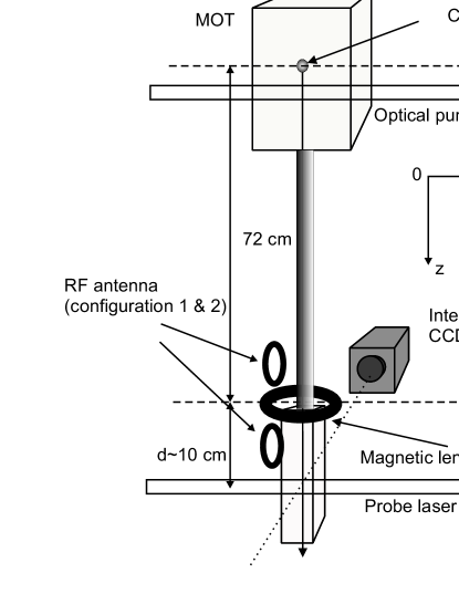
Figure 1: Schematic of the experimental set-up. The lens is made of a vertical axis coil, centered about 72 cm below the MOT center. The rf antenna is located a few cm above (configuration 1) or below (configuration 2) the lens center, with its axis along the Ox direction. The inset on the right shows 100 atomic trajectories as the cloud crosses the magnetic lens plane.

3 Experimental set-up

The experimental set-up is presented on figure 1. We prepare a cloud of cold cesium atoms in a standard magneto-optical trap. After a loading time of 1 s and a molasses phase of 15 ms, we obtain a cloud of $10^{7}$ atoms, at a temperature of 6 $\mu K$ with a 0.8 mm rms radius. The cloud is then released and falls along the vertical axis. After a 2 cm free fall, the cloud crosses a weak circularly polarized retroreflected laser resonant with the $|^{7}S_{1/2};F=4\rangle\rightarrow|^{7}P_{1/2};F^{\prime}=5\rangle$ transition. The atoms are then optically pumped in the $|F=4,m_{F}=+4\rangle$ or in the$|F=4,m_{F}=-4\rangle$ Zeeman substate depending on the sign of the circular polarization. During this polarization phase, a 5 G magnetic field is applied along the laser axis. We obtain a polarization of $70\%$ of the atoms in the aimed state, measured through an independent longitudinal Stern Gerlach analysis Guibal99 . The cloud then reaches the magnetic lens region, located about $70$ cm below the MOT center, and is focused. At the lens altitude, the cloud mean velocity is $3.7$ m/s and it constitutes a pulsed atomic beam with a narrow velocity spread $\Delta v/v\simeq 2\%$. Chromatic aberrations are thus negligible in our experiment.

The magnetic lens is made of a 66 turn square coil wrapped on a water cooled copper support. We have measured the magnetic field along the $Oz$ axis and we have checked that close to the axis the magnetic field created by the coil is equivalent to the one created by a thin circular coil with 66 turns and with a 3.15 cm radius. For the numerical simulations, we have replaced the square coil by its equivalent circular coil with the previous parameters. The current can be switched ON/OFF with a high power MOSFET. Our power supply allows us to reach a maximum current of 100 A, corresponding to a magnetic field value of 0.13 T at the coil center.

The rf antenna consists of a single turn coil of 2 $cm$ diameter, with its axis along $Ox$. The coil is in series with a 50 $\Omega$ resistive load. This resistance dominates the total impedance of the circuit and allows the matching between the antenna impedance and the 10 $W$ rf amplifier output impedance. As explained later, the rf antenna can be located above or below the lens center, leading to two experimental configurations of the magnetic lens dressed by the rf field. Furthermore the rf antenna diameter is much smaller than the magnetic lens diameter, so that the rf interaction zone is localized in a region close to the antenna position, where the rf field is strong enough to induce adiabatic transitions.

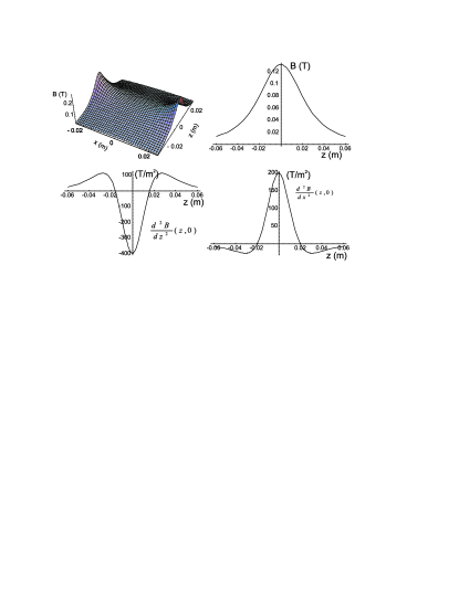
Figure 2: Space dependence of the magnetic field amplitude and its second derivatives. The magnetic field amplitude is plotted for a current in the coil of 100 A.

The detection is made by imaging on an intensified CCD camera the atom fluorescence due to the excitation by a resonant laser located at a distance $d$ below the lens center ($d$ is about $10$ cm). The magnetic field has to be switched off during the imaging time. Due to the eddy current decay time, we have to wait for 5 ms more before taking a picture. The probe is a horizontal retroreflected laser light sheet along Ox in Lin $\bot$ Lin configuration. It has a 1 mm thickness and a 10 mm width along Oy. At the same time, the probe absorption is monitored on a photodiode, allowing us to measure the cloud temperature by time of flight when the lens is switched off : the cloud temperature of 6 $\mu K$ corresponds to a time of flight width $(1/e^{2})$ of 7.9 ms. The image is taken by integrating the fluorescence with the camera during 20 ms. This duration is long enough to integrate all the atomic signal, even in presence of the longitudinal diverging effect of the lens which increases the time of flight width.

4 The magnetic lens

Before describing the lens effect in combination with a rf field, we first present the lensing effect without rf. For atoms in $|F=4,m_{F}=+4\rangle$ the magnetic potential is $\mu_{B}|B|$. The main properties of this saddle like magnetic potential are summed up on figure 2. As the magnetic field amplitude along B is maximum at the coil center, atoms are accelerated then decelerated as they cross the lens. The lens effect is caused by the parabolic part of the magnetic potential, which is proportional to the potential second derivatives. Along the vertical 0z axis, the lens acts as a diverging lens, as the potential second derivative is mainly negative. We will not investigate further this effect marechal99 . Along the radial directions, the second derivative is mainly positive and the lens acts as a converging lens. We show on figure 1 (inset) the results of a numerical simulation of the atoms trajectories as they cross the magnetic lens. Atoms can also be initially prepared in the $|m_{F}=-4\rangle$ substate and the lens becomes diverging. In the next section, we will use a rf field to resonantly spin flip the atoms while they travel through the lens, and realize a lens with a rf-controlled focal length.

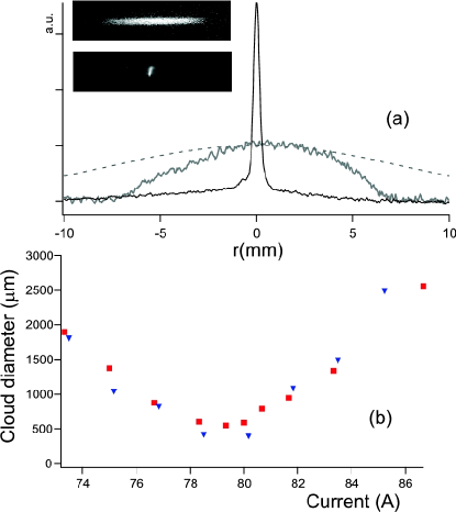
Figure 3: (a) Fluorescence images of the cloud with the lens off and on, and corresponding profiles along $Ox$ (grey and black). The current in the magnetic lens is 79 $A$. The dashed line shows the expected cloud profile in absence of truncation by the vacuum tubing. (b) Cloud diameter at the probe position (7.5 $cm$ below the lens) as function of the current in the lens. Experiment (squares) and numerical simulation (triangles).

On figure 3, we show a fluorescence picture when the cloud is focused at the probe position, located $7.5$ cm below the coil center. We show also the fluorescence image of the cloud when the lens is switched off. A gaussian fit of the profile gives a 500 $\mu m$ $1/e^{2}$ diameter of the focused cloud to be compared to the 3.1 cm diameter of the free expanding cloud (80 $cm$ of free fall at a temperature of 6 $\mu K$). The observed image without lens is not gaussian and has a measured width of only $1.3$ $cm$. The reason for this smaller than expected size is that the cloud is truncated by an aperture of $0.8$ $cm$ diameter located half way between the MOT cell and the lower glass cell; this aperture is used as a differential pumping section. Futhermore, the cloud is also truncated by the lower cell aperture of $1.6$ $cm$ diameter. As shown on figure 3(a), for a current of $79$ $A$, the cloud is focused at the probe altitude. We have measured the transverse diameter of the cloud at the probe position as a function of the current in the lens. The results are shown on figure 3(b). The cloud diameter is minimal as it is focused at the probe position. For a higher current value, the cloud is focused above the laser probe, for a lower value it is focused below the laser beam. We have compared these experimental study with a Monte Carlo numerical simulation based on the integration of 1000 classical trajectories of atoms in the magnetic potential. The 3D initial positions and velocity of the atoms are chosen at random, with the experimental gaussian distribution parameters. The numerical results reproduce well the experimental outcomes. Note that the minimal diameter value $D_{min}$ of the focused cloud, about 500 $\mu m$, is limited by the magnetic lens spherical aberrations; the initial cloud size contribution to $D_{min}$ being negligible here.

5 Magnetic lens dressed by rf

5.1 Principle

In combination with a rf field, the lens properties are strongly modified. We apply a strong monochromatic, linearly polarized rf field $\overrightarrow{B}_{rf}\cos(\omega_{rf}t)$, which couples the different sublevels $|F=4,m_{F}\rangle\leftrightarrow|F=4,m_{F}\pm 1\rangle$. The coupling creates an avoided crossing between the different sublevels, and modifies the magnetic potentials. The coupling strength is on the order of $\Omega=g_{F}\mu_{B}B_{rf}/2\hbar$ where $B_{rf}$ is the magnetic field amplitude. The exact coupling strength depends on the rf amplitude, on the relative orientation of the rf field with respect to the static field, and is $m_{F}$ dependent. In our case, the coupling dependence on the field orientation is optimal, the rf coupling field $\overrightarrow{B}_{rf}$ being perpendicular to the vertical static magnetic field. As the static magnetic field is inhomogeneous, the coupling is effective at positions where the resonance condition is fulfilled that is when $\hbar\omega_{rf}=g_{F}\mu_{B}|B|$. This condition defines an isoB surface, an atom crossing this surface is spin flipped. The correct frame to treat the problem of the coupling of the atoms with the rf field is the dressed atom picture. In presence of a rf field the nine magnetic bare states $|F=4,m_{F}\rangle$ having initial potential energies $E_{m_{F}}=m_{F}g_{F}\mu_{B}B$ give rise to nine dressed states in presence of rf with energies Colombe04 :

$$V_{m_{F}}=m_{F}\sqrt{(g_{F}\mu_{B}B-\hbar\omega_{rf})^{2}+(\hbar\Omega)^{2}}$$ (1)

The resulting adiabatic potentials are shown in a simple case on figure 4. The rf is applied in combination with an inhomogeneous magnetic field $B_{z}(0,0,z)=b^{\prime}.z$ where $b^{\prime}$ is a constant magnetic field gradient. The dressed states can be decomposed into the bare states basis $|F=4,m_{F}=-4...+4\rangle$. At the exact resonance position, the dressed states are linear superposition of all the $|m_{F}\rangle$ substates, but far from the interaction region, each dressed state is decomposed into a single bare state Colombe04 . For this reason, we have labeled on figure 4 (b) the different adiabatic potentials branches with the name of the bare state they connect to before and after the interaction region. An atom crossing the isoB plane initially in the substate $|m_{F}\rangle$ will end in the substate $|-m_{F}\rangle$. For example, atoms following adiabatically the upper potential on figure 4 (b) are transferred from the initial $|m_{F}=-4\rangle$ bare state to the final $|m_{F}=+4\rangle$ state. This spin flip has thus been made possible by the absorption of 8 rf photons (as illustrated on figure 4 (a) ) as atoms cross the resonance region.

Note that the adiabatic dressed states are eigenstates with energies given by equation (1) only for an atom at rest. Atoms cross the interaction region with a velocity of $v\simeq 4$ m/s, which can induce diabatic Landau-Zener like transitions between adiabatic states. To reduce the probability of these transitions, the rf power has to be high enough in order to increase the energy separation between the different adiabatic potentials. The probability to follow a single adiabatic potential can be described by a Landau-Zener model and will be discussed in the last part of this paper.

Figure 4: Modification of the magnetic potential in presence of a strong rf field with frequency $\omega_{rf}/2\pi$. (a) Initial potentials with $B(0,0,z)=b^{\prime}.z$. (b) The magnetic potentials are distorted into nine adiabatic potentials. The coupling takes place at the isoB plane position $Z_{rf}=\hbar\omega_{rf}/g_{F}\mu_{B}b^{\prime}$. At this position the energy separation between the different adiabatic potentials is of the order of $\hbar\Omega$

We have used this effect to realize a lens whose focal length can be tuned by the rf frequency value : if atoms are prepared in the $|^{7}S_{1/2},F=4,m_{F}=4\rangle$ state, the first part of the lens acts as a converging 2D lens. As they cross the isoB surface, atoms are adiabatically transferred to the $|^{7}S_{1/2},F=4,m_{F}=-4\rangle$ state and the second part of the lens acts as a diverging 2D lens. The combination of these two lenses realizes a doublet. By changing the rf frequency value, the isoB plane position is changed and the doublet focal length is varied. Atoms can also prepared in the $|m_{F}=-4\rangle$ sublevel, and an other doublet is realized.

Figure 5: (a) Zeeman diagram for the $|F=4,m_{F}\rangle$ states. At a rf frequency of 175 $MHz$ the coupling occurs at magnetic field values between 450 $G$ and 550 $G$. (b) Two possible experimental configurations, when the same rf frequency of 175 MHz is applied to the magnetic lens. The magnetic field profile is plotted for 80 A in the magnetic lens. Configuration 1 : The input atoms are polarized in $|m_{F}=-4\rangle$ state, and the rf antenna is located above the lens center. Configuration 2 is exactly the opposite configuration. The non linear Zeeman effect leads to a spatial dispersion of the isoB planes over 5 mm for these two experimental situations.

A difficulty arises as we want to shape magnetic potentials with strong focusing properties, so that quite intense magnetic fields are involved, and equivalently high rf frequency values. In that case, the second order Zeeman effect becomes non negligible and lifts the frequency degeneracy of the rf transitions between the different $(|m_{F}\rangle,|m_{F}+1\rangle)$ pairs. For this experimental study, we have used $\omega_{RF}/2\pi$ ranging from $100$ $MHz$ to $250$ $MHz$ corresponding to isoB field values between $370$ $G$ and $655$ $G$. At such magnetic field intensities, the second order Zeeman effect is already important and the coupling between the successive magnetic sublevels is located at different isoB plane, as shown on figure 5 (a). The figure shows that for a rf frequency of 175 MHz, the resonance takes place at a magnetic field value between 450 G for the $|m_{F}=-4\rangle\leftrightarrow|m_{F}=-3\rangle$ transition and 550 G for the $|m_{F}=4\rangle\leftrightarrow|m_{F}=3\rangle$ transition. As a consequence, the adiabatic transfer between the stretched sublevels will be efficient only if atoms cross the different isoB planes in the correct order. For an atom initially in the $|-4\rangle$ state the transfer is effective if the atom crosses a region of increasing field (positive gradient), for an atom initially in the opposite state $|m_{F}=+4\rangle$ the gradient has to be negative. We have investigated the two possibilities leading to two experimental configurations, as shown on figure 5 (b). In the first one, atoms are prepared in the $|m_{F}=-4\rangle$ state, and the rf antenna is located above the lens center. In the second one, atoms are prepared in the opposite state and the rf antenna is located below the lens center.

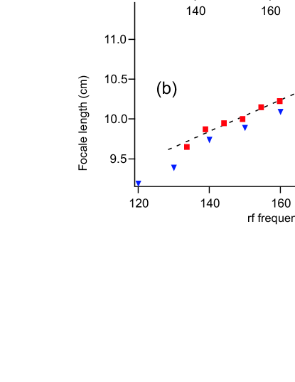
Figure 6: (a) Variation of the cloud diameter at the probe position as a function of the rf frequency. The current in the coil is 85 $A$. (b) Corresponding variation of the focal length with the rf frequency. The experimental data are deduced from (a) (see text). For (a) and (b) : Experiment (squares) , numerical simulation (triangles). The dashed lines are guides for the eye.

5.2 Experimental results

We now turn to our experimental results. A first demonstration is presented on figure 6. The current amplitude in the magnetic lens is set constant to 85 $A$. The antenna is located above the lens center (configuration 1). Atoms are prepared in the $|F=+4,m_{F}=-4\rangle$ state. The lens is first diverging, then converging, as atoms are flipped from $|m_{F}=-4\rangle$ to $|m_{F}=+4\rangle$ when they cross the rf interaction zone. The resulting lens is a converging lens, but with a longer focal length than without rf. We have measured the cloud diameter at the probe position located 10.5 $cm$ below the lens center as a function of the rf frequency. The results shown on figure 6 (a) demonstrate that the magnetic lens power can be tuned by changing only the rf frequency. The cloud is focused at the probe altitude for a rf frequency value of 170 $MHz$. The variation of the focal length with the rf frequency is presented on figure 6 (b) : it has locally a linear dependence with a slope of 125 $\mu m/MHz$. In this configuration, the focal length value is always longer than the one obtained without rf, equal to 7 $cm$ (in that case, atoms enter the lens in $|m_{F}=+4\rangle$). For figure 6(b), the experimental data have been deduced from figure 6 (a) measurements using the following observation: if the atom cloud is focused at a distance $f$ from the lens center, with a minimal spot diameter $D_{min}$, then the diameter variation with the distance $\Delta z=(f-z)$ from the focal point is given by $D(\Delta z)=\sqrt{{D_{min}}^{2}+({D_{lens}}^{2}/f^{2}){\Delta z}^{2}}$ where $D_{lens}$ is the cloud diameter at the lens position. We have checked that all our experimental measurements follow well this relation with the single parameter $D_{lens}=11$ $mm$ in correct agreement with a direct measurement (13 $mm$, see figure 3 (a)). We present also on figure 6 the results of the 3D numerical simulations. The experimental data are well reproduced by numerical simulations even if we have not introduced the non linear Zeeman effect in our simulations. Indeed, as shown on figure 5 (b), due to this effect, atoms have to travel over $l=$ 5 $mm$ to be flipped from $|m_{F}=-4\rangle$ to $|m_{F}=+4\rangle$. This distance remains nevertheless small compared to the static field extension (5 $cm$) and can be neglected in numerical simulations. For these calculations, the rf effect is taken into account by a sudden change of the force sign, as atoms cross the isoB plane.

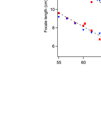
Figure 7: Evidence for a rf-induced increase in the lens power. The focal length is plotted versus the coil current for configuration 2. The rf frequency is set to 210 $MHZ$. Experimental data (squares) = with rf, (rounds)= no rf, and numerical calculations (triangles). The dashed lines are guides for the eye. (The increase of the focusing power of the lens with the rf is evident from a comparison of the two sets of points.)

Configuration 1 is also interesting since it can be used to realize a fast atomic shutter using no moving mechanical element. Atoms initially prepared in the $|m_{F}=-4\rangle$ state are expelled from the vertical axis when the rf-field is switched off. The atomic signal at the probe beam position is then negligible. When the rf-field is switched on, an intense signal appears. The switching time is limited by the second order Zeeman effect, which is responsible for a shift between the isoB planes coupling the successive magnetic states (see figure 5). If we call $l$ the distance between the two extreme planes, the switching time is equal to $\tau=l/v$ where $v$ is the mean atomic beam velocity. For this experiment, with $l\simeq 5$ $mm$ (see figure 5(b)) and $v=4$ $m/s$ we got $\tau\simeq 1$ $ms$. To have a shorter switching time, an antenna working at a smaller frequency could be placed in the lower field region, where the second order Zeeman effect is much smaller. An other possibility is to use atoms having no hyperfine structure and therefore no non linear Zeeman effect, like ${}^{52}Cr$, which is particularly well suited for atomic nanofabrication Meschede2003 .

On figure 7, we show the results for configuration 2: the rf antenna is located below the lens center and atoms are initially prepared in the $|m_{F}=+4\rangle$ state. For the experimental demonstration, the frequency was set to 210 $MHz$, and we have measured the cloud diameter at the probe position, located 8 $cm$ below the lens center, as a function of the current in the magnetic lens. We have extracted from the data the effective variation of the focal length as described for configuration 1. With the rf ON, the cloud is focused 8 $cm$ below the lens center for a current of 60 $A$. Without rf, the focal value jumps to 12 $cm$ for the same current. Numerical calculations reproduce well the experimental observations.

In configuration 2, the ’dressed lens’ is always more focusing than the ’bare lens’, and the focal length decreases as the rf frequency increases. As shown by further simulations, the lens can be changed from a converging lens to a converging mirror, by changing only the rf frequency. For example, we have calculated numerically that for a current of 100 A in the lens, and a rf frequency higher than 380 $MHz$, the dressed lens acts as a converging mirror. Such high rf frequencies are beyond the values that we can reach with our rf supply. This configuration is similar to the one used in Bloch2001 where a resonator for atoms was demonstrated.

5.3 Rf power requirements, Landau Zener criterion

Atoms cross the interaction zone with a velocity $v\simeq 4$ $m/s$ giving rise to a non adiabatic probability transition. The probability to have a single non adiabatic transition between two adjacent states $|m_{F}\rangle$ and $|m_{F}+1\rangle$ is given by the Landau Zener formula Laundau32 :

$$P_{LZ}=e^{-2\pi\Gamma(m_{F},m_{F}+1)}$$ (2)

with

$$\Gamma(m_{F},m_{F}+1)=\frac{\hbar\Omega^{2}(m_{F},m_{F}+1)}{g_{F}\mu_{B}b^{\prime}v}$$ (3)

where $b^{\prime}$ is the magnetic gradient and $\Omega(m_{F},m_{F}+1)$ is the Rabi frequency between $|m_{F}\rangle$ and $|m_{F}+1\rangle$. At low field value, the coupling strength is given by Ketterle96

$$\Omega(m_{F},m_{F}+1)=\frac{\mu_{B}g_{F}}{4\hbar}B_{rf}\sqrt{F(F+1)-m_{F}(m_{F}+1)}$$ (4)

We have checked that even at our magnetic field value (around 600 $G$) where the non linear Zeeman effect is non negligible, couplings are not modified by more than 10 % and we can use equation (4) to calculate them. On the other hand, the transitions between the different $|m_{F}\rangle\leftrightarrow|m_{F}+1\rangle$ are spatially separated and occur one after the other due to the same effect. The atom transfer efficiency from $|-4\rangle$ to $|+4\rangle$ is thus given by the product of the probabilities of the successive transitions between adjacent $|m_{F}\rangle$ substates and is given by :

$$P_{4\leftrightarrow(-4)}=\prod^{m_{F}=+3}_{m_{F}=-4}{(1-e^{-2\pi\Gamma(m_{F},m_{F}+1)})}$$ (5)

Using equation (3) and (4), we obtain that atoms are adiabatically transferred if $h\Omega^{2}\gg\mu_{B}g_{F}vb^{\prime}$. For $v=4$ $m/s$ and $b^{\prime}=200$ $G/cm$ we obtain that $P_{4\leftrightarrow(-4)}>95\%$ for $B_{rf}>200$ $mG$.

We turn now to the exact calibration of the rf magnetic field amplitude $B_{rf}$. We have verified that our single turn antenna, in series with a 50 $\Omega$ resistance, is well adapted to the rf supply output impedance: the measured rf reflected power is less than 10%, showing that the antenna inductance gives a negligible contribution to the total circuit impedance. We can then calculate the AC current amplitude in the rf antenna for a given power, and the magnetic field $B_{rf}$. At a power of 10 $W$, we estimate that $B_{rf}=175$ $mG$ at the cloud center (1 $cm$ away from the rf coil center). Note that the adaptation procedure works only if the rf antenna diameter is small, otherwise the inductance increases and the rf power is reflected by the antenna, so that there is almost no current in the antenna. Our rf antenna has a diameter of 2 $cm$. Due to its rather small size compared to the magnetic lens coil size, the antenna position has to be adjusted to the mean rf frequency value, in order to match its altitude with the isoB plane position and thus to maximize the coupling strength. In fact, the magnetic field amplitude $B_{rf}$ is not well defined due to the transverse extension of the cloud. Indeed, at the entrance of the magnetic lens, the cloud radius is of the order of 4 mm (radius of a sphere containing 80 $\%$ of the atoms). For a rf antenna located at 1 $cm$ from the cloud centre, the rf magnetic field amplitude varies between 312 $mG$ and 97 $mG$ over the cloud extension, and is equal to 175 $mG$ at the cloud centre as found before. This central value gives a good estimation of the mean magnetic field seen by the atoms, and can be used for our qualitative discussion on power requirements.

We have measured the transfer probability as a function of the rf power (figure 8). Atoms are initially polarized in the $|m_{F}=-4\rangle$ state. The probability is evaluated by measuring the number of atom focused at the probe position for a given rf power, normalized by the number of atom focused at the probe position, with no rf, when atoms are initially polarized in $|m_{F}=+4\rangle$ state. For a power of 10 W the transfer is close to 100%. The data are in good agreement with the theoretical estimate given by equation (5).

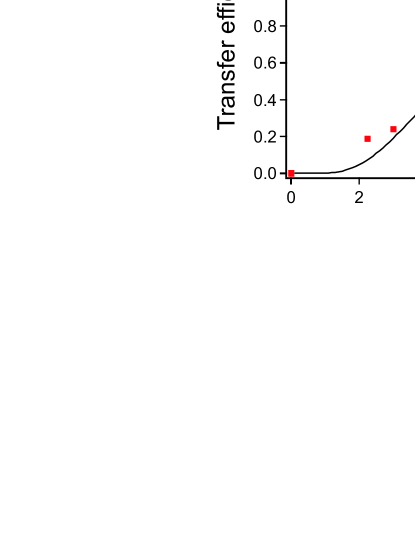
Figure 8: Transfer efficiency as a function of the rf power. The rf frequency was fixed to 130 $MHz$, the current in the lens to 95 A. Atoms are initially polarized in $|m_{F}=-4\rangle$ state (configuration 1) and we measure the number of atoms focused at the probe position and normalized it (see text). The black line is obtained from 5, the scaling between $\Omega^{2}$ and the rf power being given by the experimental calibration.

6 Conclusion

In conclusion, we have demonstrated a new type of atomic lens by combining a permanent magnetic lens with a rf field. The focal length of this atomic lens can be finely tuned with the rf frequency value and the lens can be changed from a less converging to a more converging lens, and even could be changed to a converging mirror. The combination of rf fields with static inhomogeneous magnetic fields gives new properties to traditional atom optics elements like lenses, mirrors and magnetic guides. The use of frequency combs or of rf sweeps can add even more possibilities to generate more complex potentials Courteille06 . We think that this innovative procedure can join the atom optics toolbox since further improvements along this scheme should result in the development of high quality coherence preserving atomic adaptative lenses and mirrors. Futhermore the rf dressing procedure can be readily combined with the well developed integrated atom chip technology, to add coherent controls to magnetic atoms chips zimmermann07 .

Acknowledgments: LPL is Unité Mixte (UMR 7538) of CNRS and of Université Paris Nord. We acknowledge financial support from Conseil Régional d’Ile-de-France (Contrat Sesame), Minist re de l’Enseignement Sup rieur et de la Recherche, European Union (Feder-Objectif 2), and IFRAF (Institut Francilien de Recherche sur les Atomes Froids - MOCA project). We thank J.M. Fournier for many fruitful discussions.

References

- (1) O. Zobay and B. M. Garraway. Phys. Rev. Lett., 86(7):1195–1198, Feb 2001.
- (2) O. Zobay and B. M. Garraway. Phys. Rev. A, 69(2):023605, 2004.
- (3) Y. Colombe, E. Knyazchyan, O. Morizot, B. Mercier, V. Lorent, and H. Perrin. EPL (Europhysics Letters), 67(4):593–599, 2004.
- (4) I. Lesanovsky, T. Schumm, S. Hofferberth, L. M. Andersson, P. Krüger, and J. Schmiedmayer. Phys. Rev. A, 73(3):033619, 2006.
- (5) T. Fernholz, R. Gerritsma, P. Krüger, and R. J. C. Spreeuw. Phys. Rev. A, 75(6):063406, 2007.
- (6) Ph. W. Courteille, B. Deh, J. Fortágh, A. Günther, S. Kraft, C. Marzok, S. Slama, and C. Zimmermann. Journal of Physics B: Atomic, Molecular and Optical Physics, 39(5):1055–1064, 2006.
- (7) E A Hinds and I G Hughes. J. Phys. D, 32(18):R119–R146, 1999.
- (8) E. Maréchal, S. Guibal, J.-L. Bossennec, R. Barbé, J.-C. Keller, and O. Gorceix. Phys. Rev. A, 59(6):4636–4640, Jun 1999.
- (9) Tanguy Miossec, René Barbé, Jean-Claude Keller, and Olivier Gorceix. Optics Communications, 209(4-6):349–362, 2002.
- (10) É. Maréchal, S. Guibal, J.-L. Bossennec, M.-P. Gorza, R. Barbé, J.-C. Keller, and O. Gorceix. Eur. Phys. J. D, 2:195–198, 1999.
- (11) D Meschede and H Metcalf. Journal of Physics D: Applied Physics, 36(3):R17–R38, 2003.
- (12) Immanuel Bloch, Michael Köhl, Markus Greiner, Theodor W. Hänsch, and Tilman Esslinger. Phys. Rev. Lett., 87(3):030401, Jul 2001.
- (13) L. Landau. Phys. Z. Sowjet Union, 46(2), 1932.
- (14) W. Ketterle and N. J. van Druten. Adv. At. Mol. Opt. Phys., 37, 1996.
- (15) Jozsef Fortagh and Claus Zimmermann. Reviews of Modern Physics, 79(1):235, 2007.