The instability of counter-propagating kernel gravity waves in a constant shear flow

Abstract

The mechanism describing the recently developed notion of kernel gravity waves (KGWs) is reviewed and such structures are employed to interpret the unstable dynamics of an example stratified plane parallel shear flow. This flow has constant vertical shear, is infinite in the vertical extent, and characterized by two density jumps of equal magnitude each decreasing successively with height, in which the jumps are located symmetrically away from the midplane of the system. We find that for a suitably defined bulk-Richardson number there exists a band of horizontal wavenumbers which exhibits normal-mode instability. The instability mechanism closely parallels the mechanism responsible for the instability seen in the problem of counter-propagating Rossby waves. In this problem the instability arises out of the interaction of counter-propagating gravity waves. We argue that the instability meets the Hayashi-Young criterion for wave instability. We also argue that the instability is the simplest one that can arise in a stratified atmosphere with constant shear flow. The counter propagating gravity waves mechanism detailed here explains why the Rayleigh criteria for shear flow instability in the unstratified case does not need to be satisfied in the stratified case. This illustrates how the Miles-Howard theorem may support destabilization through stratification. A normal mode analysis of a foamy layer consisting of two density jumps of unequal magnitude is also analyzed. The results are considered in terms of observations made of sea-hurricane interfaces.

I Introduction

Shear flows and the variety of instabilities they precipitate are difficult processes to conceptualize despite over a century of inquiry. The two different interpretative tools available are the theory of counter-propagating Rossby Waves (CRWs)bretherton ; heifetz99 ; heifetzCRW and classic over-reflection theory (O-R)lindzen and these, in turn, have been shown to be equivalent in rationalizing non-stratified shear flows nili_n_eyal . While O-R theory can be used to interpret stratified shear flows, the CRW approach cannot be used in the same way because the basic building-block structures of CRW theory, namely kernel Rossby waves (KRWs)heifetz99 , do not describe buoyancy. However a formulation in the spirit of CRWs has been recently developed to include the effects of stratificationHHUL07 . The basic building blocks of this generalized wave kernel approach, namely kernel Rossby-gravity waves (KRGWs), turn into KRWs when buoyancy effects are absent.

We apply this approach to an example stratified shear flow in order to observe how the mechanics of this interpretive tool unfolds. The geometry is an infinite atmosphere composed of divergence free fluids in a globally constant shear flow. The atmosphere is comprised of fluids of three densities where the two density jumps of equal magnitude are located symmetrically away from the (nominal) midplane of the atmosphere.

The important matter to recognize is that because there is no-basic vorticity gradient there will be no Rossby waves present at the density interfaces. In this way the KRGW building blocks of the generalized theory will reduce to what we call here kernel gravity waves or “KGWs” for short. The KGW concept has antecedents tracing back to the work of Sakai (1989)sakai in which density-shear disturbances in a shallow-water model are analyzed in terms of physical wave coordinates. The problem investigated by Sakai sakai cast the emerging instabilities in terms of a wave interaction mechanism in which counter-propagating waves influence each other from a distance. Baines and Mitsudera (1994)BM94 further generalize these concepts as fitting into a more unified mechanism of shear flow instabilities. As an example they show how the classic Holmboe instability holmboe62 may be rationalized in terms of the interaction between the waves on separated density and vorticity surfaces.

In the problem we examine here there will be four KGWs, two associated at each interface. Of the two at each interface one will travel faster than the local flow speed while the other will be slower than the local flow speed. Of the four modes only two modes, each counter-propagating with respect to the local flow speed of its respective interface, may transit into a stable-unstable pair. We find that for given values of the bulk-Richardson number (defined below) there will always be a band of horizontal wavenumbers which admit normal-mode instability. The KGW analysis performed here shows something quite interesting: the mechanics of the instability bears strong resemblance to the mechanics responsible for the instability in the classic CRW problem heifetz99 and, furthermore, become mathematically equivalent in the limit of small horizontal wavelengths. Thus despite the fact that in this problem there are no Rossby waves present (i.e. as edge waves) buoyancy oscillations in relative motion with each other interact dynamically in such a way that it can induce instability in the same way that CRWs produce instability in Rayleigh’s classic problem heifetzCRW ; Rayleigh1880 .

Further reflection also shows that onset of instability satisfies the criterion of Hayashi & Young (1987)hayashi_young . The stability criterion states that for flows of this sort a transition into linear stability occurs if there are individual waves in the flow which: (i) propagate opposite to each other, (ii) have almost the same Doppler-shifted frequency and (iii) can interact with one anothersakai . Indeed in the current problem we see that instability develops out of KGWs which counter-propagate at their respective interface and through their action-at-a-distance interaction heifetz99 trigger a transition into instability for given values of a bulk Richardson number.

We note that the work of CaulfieldCaulfield94 , which is an investigation of a variation of Holmboe’s problem holmboe62 , contains as a special limiting case the instability uncovered here. In that study a density configuration exactly like the one considered here is analyzed. The difference is that there exists symmetrically placed jumps in the background vorticity resembling the classic Rayleigh profile. These vorticity jumps, located at $z=\pm d$, are at points some distance removed from the density jumps located at $z=\pm h$. In general many types of modes appear in this problem. Of these, the ones referred to as Taylor modes may be shown to limit to the type of modes studied here when $d\gg h$. However, this limiting procedure was not performed and the qualitative significance of this instability had not been appreciated at the time.

It is important to note here that the three-layer density configuration we consider in this work has been proposed to be qualitatively applicable to the question of drag reduction in rough seas driven by hurricane force winds newell ; powell . The middle “foamy” layer Miki_2007 serves to dissipate energy and transfer momentum between the air and sea. Theoretical work in problems with this sort of stratification craik ; Miki_2007 consider uniform velocity profiles within each of the three layers but otherwise different between them. In this way we see the physical results derived from this study as complementary to these cited works because the velocity profile we consider has uniform shear as opposed to (effective) delta-function jumps in the shear.

This work is organized according to the following prográmme. In Section II we present and review the formulation derived in Harnik et al. (2007)HHUL07 . In Section III we work through the theory for KGWs in an atmosphere of constant shear and a single density jump. As a matter of review we expend some effort describing the mechanics of the KGW. In Section IV we introduce the problem of two density jumps of equal magnitude, analyze its normal modes, motivate its generalized formulation as an initial value problem and then argue for the rationalizion of its unstable dynamics. We find that when the system is unstable the mechanics of the modes closely parallels the processes occurring for unstable CRWs heifetzCRW under conditions where the layers are not too close to one another. We also spend a few words to rationalize the instability in terms of the criterion of Hayashi & Young (1987) and Sakai (1989) hayashi_young ; sakai . In Section V we study the normal-mode response of this configuration when the layer is considered foamy. This corresponds to the problem considered in Section IV but where, instead, the density jumps are not of equal magnitude. As in Shtemler et al. (2007) Miki_2007 , the density ratio of successive layers is measured by the parameter $\delta$ in which $0<\delta<1$. In comparison to the results of Section IV (where $\delta\approx 1$), we find that the range of unstable wavenumbers and the peak growth rate shrinks as $\delta$ approaches zero. We also find that the modes are propagatory when they become unstable. Section VI summarizes our results and we show that the instability does not violate the Miles-Howard Theoremmiles61 ; howard61 . We also suggest that this instability, manifesting itself under conditions that are classically considered to be stably stratified, may be the simplest one possible which can destabilize a plane-Couette profile. We conjecture upon the results of this study and its relationship to the problem of sea surface foam layers observed in hurricanes.

II Basic formulation: a review

We begin the analysis by recasting the equations of linearized motion in terms of the formalism outlined in Harnik et al. (2007)HHUL07 . Namely, the primitive equations of motion describing Boussinessq incompressible 2D flow are

$$\frac{Du}{Dt} = -\bar{U}_{z}w-\frac{1}{\rho_{0}}\frac{\partial P}{\partial x},$$ (1)

$$\frac{Dw}{Dt} = -\frac{1}{\rho_{0}}\frac{\partial P}{\partial z}+b,$$ (2)

together with the equation of continuity and incompressibility

$$\frac{Db}{Dt} = -wN^{2},$$ (3)

$$\frac{\partial u}{\partial x}+\frac{\partial w}{\partial z} = 0.$$ (4)

The variables $u$ and $w$ are the horizontal ($x$) and vertical velocities ($z$) (respectively). The horizontal mean flow is $\bar{U}$ and where we have defined $\bar{U}_{z}\equiv\frac{dU}{dz}$ as the mean shear together with $\frac{D}{Dt}\equiv(\partial_{t}+\bar{U}\partial_{x})$. The density $\rho$ is cast in terms of the variable $b\equiv-g\rho/\rho_{0}$ and where

$$N^{2}\equiv-\frac{g}{\rho_{0}}\frac{d\rho}{dz}=\frac{d\bar{b}}{dz}.$$

Because the flow is incompressible the evolution of the density $\rho(z,t)$ may be equivalently traced by the motion of some material invariant. In this case we follow the vertical displacement $\zeta$ of a fluid parcel which was otherwise at rest. The undisturbed density profile is assumed to have a vertical variation of some sort and, thus, the displacement may be easily associated with clearly identifiable surfaces. Thus, as was demonstrated in Harnik et al. (2007)HHUL07 , we shall write the equations of motion in terms of the evolution of the vorticity and vertical displacement as

$$\frac{Dq}{Dt} = -\bar{q}_{z}w+\frac{\partial b}{\partial x},$$ (5)

$$\frac{D\zeta}{Dt} = w(x,z),$$ (6)

where $\bar{q}_{z}\equiv-\bar{U}_{zz}$, $b=-\bar{b}_{z}\zeta$ and where,

$$w(x,z)=\frac{\partial\psi}{\partial x},\qquad u(x,z)=-\frac{\partial\psi}{\partial z},$$ (7)

in which we have expressed velocities in terms of the usual stream function formulation of 2D incompressible problems and where the vorticity $q$ is

$$q=\frac{\partial w}{\partial x}-\frac{\partial u}{\partial z}=\nabla^{2}\psi$$ (8)

III Single density jump

From here on out we assume the background flow state to be a constant shear (i.e. $\bar{q}_{z}=\bar{U}_{zz}=0$). We examine here a single density interface located at the position $z=0$. The basic state density is written as

$$\bar{\rho}=\rho_{0}+{\Delta\bar{\rho}}H(z),$$ (9)

where $H$ is the Heaviside function. The equations of motion now become,

$$(\partial_{t}+U\partial_{x})q = (g\Delta\rho/\rho_{0})\partial_{x}\zeta\delta(z),$$ (10)

$$(\partial_{t}+U\partial_{x})\zeta = w(x,0).$$ (11)

(10) says that the vorticity ought to also have a delta function dependence. Thus we make the ansatz

$$q=\hat{q}(x,t)\delta(z).$$

To proceed, we assume that all variables have a Fourier decomposition in the $x$ direction, that is to say

$$\sim e^{ikx}+{\rm c.c.}$$

where $k$ is the horizontal wavenumber. We begin with the solution to the streamfunction. As the ansatz indicates, away from the interfaces the vorticity is zero. Thus it means that one formally writes the solution to the stream function equation (8) as

$$\psi=\hat{q}(x,t)\int_{-\infty}^{\infty}G(z,z^{\prime})dz^{\prime},$$ (12)

since $\nabla^{2}G=(\partial_{z}^{2}-k^{2})G(z,z^{\prime})=\delta(z-z_{0})$, and because this geometry is so simple the solution for $\psi$ is

$$\psi=-\frac{\hat{q}}{2k}e^{-k|z-z_{0}|}.$$ (13)

Implicit in the construction of this solution is that (a) the vertical velocity, $w=\partial_{x}\psi$ is continuous across the interface and (b) the vorticity delta function results from the jump in u across $z_{0}$. We are now in a position to put these expression explictly into the equations of motion above. Thus one has, after shaking out algebraic factors and the solution ansatz,

$$(\partial_{t}+ikU_{0})\hat{q} = ik\frac{g\Delta\rho}{\rho_{0}}\zeta,$$ (14)

$$(\partial_{t}+ikU_{0})\zeta = -\frac{i}{2}\hat{q},$$ (15)

where $U_{0}=U(z=0)$. Let us suppose that $U_{0}=0$ for this problem. Let us define the gravity wave speed $c_{g}\equiv N/k=\sqrt{-\frac{g\Delta\bar{\rho}}{2\rho_{0}k}}$. Provided that $\Delta\bar{\rho}<0$ (stably stratified) then the gravity wave speed is real - and this we assume henceforth. We find that the above two equations appear rewritten as

$$\partial_{t}\hat{q} = -2ik^{2}c_{g}^{2}\zeta,$$ (16)

$$\partial_{t}\zeta = -\frac{i}{2}\hat{q}.$$ (17)

The above is the ode system, in time, describing the evolution of simple classical Rayleigh-Taylor modes. Note that this system is normal as far as the operators are concerned Schmid . We can further proceed by defining new quantities through the relationship

$$\zeta_{\pm}=\frac{1}{2}\left(\zeta\pm\frac{1}{2kc_{g}}\hat{q}\right),$$ (18)

revealing to us the simplified system

$$(\partial_{t}+ikc_{g})\zeta_{+} = 0,$$ (19)

$$(\partial_{t}-ikc_{g})\zeta_{-} = 0.$$ (20)

A normal mode analsysis may proceed from here by assuming $e^{-ikct}$ dependence upon all the solutions in which $c$ is the wavespeed. It is quite straightforward to establish that the eigenmodes for this system are described by

$$(c-c_{g})\zeta_{+} = 0,$$ (21)

$$(c+c_{g})\zeta_{-} = 0.$$ (22)

For the sake of this illustration let us consider the propagation of the $\zeta_{+}$ mode which propagates at speed $c=c_{g}$. To study $\zeta_{+}$ in isolation means setting $\zeta_{-}$ to zero which, in turn, means that,

$$\zeta\sim\hat{q}.$$

In other words, the disturbance height is positively correlated with the local vorticity.

Referring to Fig. 1 we depict this situation for a stably stratified density profile. We focus our attention to the section of fluid located between the two triangles (representing the peak and trough of the wave). The fluid layer has been disturbed from its equilibrium configuration (denoted by dashed lines) in such a way that it looks like a lever arm out of balance with the fulcrum denoted with a solid filled circle. One’s intuition instructs that in this condition the lever arm has the tendency to rotate in a counter clockwise sense (positive vorticity) about this fulcrum point. This is simply the fluid’s tendency to flatten out. Thus the out-of-equilibrium arrangement equates to a local creation of vorticity, i.e. a positive time rate of change of vorticity there (shown with a dashed counter-clockwise arrow on the graph). However, the already preexisting vorticity of this disturbance (shown with solid counter-clockwise arrow) causes, for example, the position of the fulcrum point to move up because the velocity field there points upwards (solid arrow). As this section of fluid responds, vertical velocity fields also develop at the positions of the triangles in proportion to the amount of vorticity being generated at the fulcrum (denoted with the dashed vertical arrows above and below the left and right triangles respectively).

In the panel immediately below we see what happens after one quarter cycle: the positive time rate of change of vorticity at the point which was once the fulcrum has turned into a positive vorticity and the fulcrum point has turned into the maximum height of the wave. As this occurred, the position of the triangles have moved correspondingly. In this way the entire pattern has shifted to the right. The mechanics of the oppositely propagating mode, $\zeta_{-}$, are recovered in a simple way: $q$ and correspondingly $w$ are reversed and hence $\partial_{t}q$ and $\partial_{t}\zeta$ are then also reversed and then, consequently, the pattern moves to the left. Note that in this case $\zeta_{-}$ and $q$ are in phase.

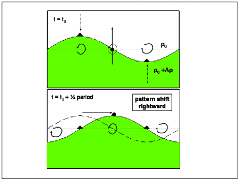
Figure 1: A mechanism schematic for the single kernel gravity wave $\hat{\zeta}_{+}$ in which positive disturbances are correlated with positive vorticity disturbances. Fluid of two differing densities are disturbed with sinusoidal profile. The corresponding negative/positive vorticity profile is represented by solid clockwise/counterclockwise arrows. Restricting attention to between the two labeled triangles in the top panel, the density arrangement looks like a displaced lever arm in a gravitational field whose 1D pivot (fulcrum) point is located at the position of the solid circle. This physically represents the tendency for the fluid to flatten out. The lever arm effect has a tendency to create positive vorticity about the fulcrum (dashed counterclockwise arrow). Concurrently, the preexisting flow due to the disturbance profile (solid clockwise/counterclockwise arrows) causes this point to rise upwards (solid arrow). As vorticity is created there, it also begins to create a velocity field at the triangles causing those positions to move (according to the manner denoted by the dashed arrows). By the time the fulcrum point reaches its peak, due to the lever arm effect there now exists positive vorticity in this local patch of the fluid after one quarter period. The pattern consequently shifts rightward (bottom panel).

IV Two density jumps in a globally constant shear

We now consider a situation in which there are two density jumps located symmetrically at a distance $h$ away from the position $z=0$. Thus,

$$\bar{\rho}=\Delta\bar{\rho}_{1}H(z-z_{1})+\rho_{0}+\Delta\bar{\rho}_{2}H(z-z_{2}),$$ (23)

where the locations $z_{1,2}$ are given by

$$z_{1}=h+\zeta_{1}(x,t),\qquad z_{2}=-h+\zeta_{2}(x,t).$$

We assume a configuration in which the shear is globally constant so that $\bar{U}=\Lambda z$ implying that $\bar{q}_{z}=0$. We further say that $\Lambda\equiv U/h$ where $U$ is the magnitude of the background flow at $z=\pm h$. We have written matters in this way to always make sure that at $z=h$ the wind is easterly (positive), in other words, we will assume that $U>0$ without loss of generality. Also, as before, we shall consider stably stratified configurations so that both $\Delta\bar{\rho}_{1}<0$ and $\Delta\bar{\rho}_{2}<1$.

Inspection shows that this form of the unperturbed density spawns delta function forms for the vorticity as we encountered before. In other words it means that we write

$$q=\hat{q}_{1}(x,t)\delta(z-z_{1})+\hat{q}_{2}(x,t)\delta(z-z_{2}).$$ (24)

Putting these forms into the governing equations (5-6) and assuming the single-wave Fourier ansatz

$$\{\hat{q}_{1},\zeta_{1},\hat{q}_{2},\zeta_{2},\psi\}^{\bf T}=\{\tilde{q}_{1},\tilde{\zeta}_{1},\tilde{q}_{2},\tilde{\zeta}_{2},\tilde{\psi}\}^{\bf T}e^{ikx}+{\rm c.c.},$$ (25)

we find the following four equations to emerge,

$$\left(\frac{\partial}{\partial t}+ikU\right)\tilde{q}_{1} = ikh\tilde{N}^{2}_{{}_{1}}\tilde{\zeta}_{1},$$ (26)

$$\left(\frac{\partial}{\partial t}+ikU\right)\tilde{\zeta}_{1} = \tilde{w}(h),$$ (27)

$$\left(\frac{\partial}{\partial t}-ikU\right)\tilde{q}_{2} = ikh\tilde{N}^{2}_{{}_{2}}\tilde{\zeta}_{2},$$ (28)

$$\left(\frac{\partial}{\partial t}-ikU\right)\tilde{\zeta}_{2} = \tilde{w}(-h).$$ (29)

with $\tilde{N}^{2}_{{}_{1,2}}\equiv-\frac{g\Delta\rho_{1,2}}{h\rho_{0}}$. We refer the reader to Appendix A for a detailed derivation of these equations from first principles. The solution to the streamfunction, i.e. (63), is rewritten here:

$$\tilde{\psi}=-\frac{\tilde{q}_{1}}{2k}e^{-k|z-h|}-\frac{\tilde{q}_{2}}{2k}e^{-k|z+h|}.$$ (30)

Since $\tilde{w}\rightarrow ik\tilde{\psi}$ we may explicitly write the vertical velocity at the levels $z=\pm h$

$$\tilde{w}(h)=-\frac{i\tilde{q}_{2}}{2}e^{-2kh}-\frac{i\tilde{q}_{1}}{2},\qquad\tilde{w}(-h)=-\frac{i\tilde{q}_{2}}{2}-\frac{i\tilde{q}_{1}}{2}e^{-2kh}.$$

Thus, we have finally

$$\left(\frac{\partial}{\partial t}+ikU\right)\tilde{q}_{1} = -2ik^{2}c_{g1}^{2}\tilde{\zeta}_{1},$$ (31)

$$\left(\frac{\partial}{\partial t}+ikU\right)\tilde{\zeta}_{1} = -i\frac{\tilde{q}_{2}}{2}e^{-2kh}-i\frac{\tilde{q}_{1}}{2},$$ (32)

$$\left(\frac{\partial}{\partial t}-ikU\right)\tilde{q}_{2} = -2ik^{2}c_{g2}^{2}\tilde{\zeta}_{2},$$ (33)

$$\left(\frac{\partial}{\partial t}-ikU\right)\tilde{\zeta}_{2} = -i\frac{\tilde{q}_{2}}{2}-i\frac{\tilde{q}_{1}}{2}e^{-2kh},$$ (34)

in which

$$c_{g1}^{2}\equiv-\frac{g\Delta\rho_{1}}{2\rho_{0}k},\qquad c_{g2}^{2}\equiv-\frac{g\Delta\rho_{2}}{2\rho_{0}k}.$$

We may recast the equations of motion in this case in terms of the individual “kernel” waves that propagate on each interface (see Section III and Harnik et al. 2007HHUL07 ). This re-formulation will be beneficial because it will show us transparently how these individual waves interact with one another. To that end we define the correlated/anticorrelated (“$\pm$”) wave quantities appropriate to each surface,

$$\tilde{\zeta}_{{}_{1\pm}} = \frac{1}{2}\left(\tilde{\zeta}_{1}\pm\frac{1}{2kc_{g1}}\tilde{q}_{1}\right),$$ (35)

$$\tilde{\zeta}_{{}_{2\pm}} = \frac{1}{2}\left(\tilde{\zeta}_{2}\pm\frac{1}{2kc_{g2}}\tilde{q}_{2}\right),$$ (36)

substituting these definitions into (38) along with the observation that

$$\frac{\tilde{q}_{1}}{2kc_{{}_{g1}}}=\tilde{\zeta}_{{}_{1+}}-\tilde{\zeta}_{{}_{1-}},\qquad\frac{\tilde{q}_{2}}{2kc_{{}_{g2}}}=\tilde{\zeta}_{{}_{2+}}-\tilde{\zeta}_{{}_{2-}},$$

and after some reshuffling of terms this results in,

$$\left(\frac{\partial}{\partial t}+ikc_{{g1}}+ikU\right)\tilde{\zeta}_{{}_{1+}} = -ik\beta_{2}\Bigl{(}\tilde{\zeta}_{{}_{2+}}-\tilde{\zeta}_{{}_{2-}}\Bigr{)},\ \$$ (37a)

$$\left(\frac{\partial}{\partial t}-ikc_{{g1}}+ikU\right)\tilde{\zeta}_{{}_{1-}} = -ik\beta_{2}\Bigl{(}\tilde{\zeta}_{{}_{2+}}-\tilde{\zeta}_{{}_{2-}}\Bigr{)},\ \$$ (37b)

$$\left(\frac{\partial}{\partial t}+ikc_{{g2}}-ikU\right)\tilde{\zeta}_{{}_{2+}} = -ik\beta_{1}\Bigl{(}\tilde{\zeta}_{{}_{1+}}-\tilde{\zeta}_{{}_{1-}}\Bigr{)},\ \$$ (37c)

$$\left(\frac{\partial}{\partial t}-ikc_{{g2}}-ikU\right)\tilde{\zeta}_{{}_{2-}} = -ik\beta_{1}\Bigl{(}\tilde{\zeta}_{{}_{1+}}-\tilde{\zeta}_{{}_{1-}}\Bigr{)},\ \$$ (37d)

where

$$\beta_{1}=c_{{}_{g1}}\frac{e^{-2kh}}{2};\qquad\beta_{2}=c_{{}_{g2}}\frac{e^{-2kh}}{2}.$$

Provided that $c_{{g1}}$ and $c_{{g2}}$ are real (that is to say, that the density succesively gets smaller with increased height) , the structures $\tilde{\zeta}_{{}_{1\pm}},\tilde{\zeta}_{{}_{2\pm}}$ are each interpreted as pairs of kernel gravity wave modes at their respective surfaces. Note that $\tilde{\zeta}_{{}_{1+}}$ and $\tilde{\zeta}_{{}_{2-}}$ are waves which move in the same direction as the local flow speed (at their respective levels) while $\tilde{\zeta}_{{}_{1-}}$ and $\tilde{\zeta}_{{}_{2+}}$ move against the local flow speed. The latter two structures are central actors when instability develops (see below).

IV.1 Normal Modes - and Recasting

Now we can take this further and assume $e^{-ikct}$ solutions and inquire about the normal mode behavior of (37), revealing

$$(c-c_{{g1}}-U)\tilde{\zeta}_{{}_{1+}} = \beta_{2}\Bigl{(}\tilde{\zeta}_{{}_{2+}}-\tilde{\zeta}_{{}_{2-}}\Bigr{)},$$ (38a)

$$(c+c_{{g1}}-U)\tilde{\zeta}_{{}_{1-}} = \beta_{2}\Bigl{(}\tilde{\zeta}_{{}_{2+}}-\tilde{\zeta}_{{}_{2-}}\Bigr{)},$$ (38b)

$$(c-c_{{g2}}+U)\tilde{\zeta}_{{}_{2+}} = \beta_{1}\Bigl{(}\tilde{\zeta}_{{}_{1+}}-\tilde{\zeta}_{{}_{1-}}\Bigr{)},$$ (38c)

$$(c+c_{{g2}}+U)\tilde{\zeta}_{{}_{2-}} = \beta_{1}\Bigl{(}\tilde{\zeta}_{{}_{1+}}-\tilde{\zeta}_{{}_{1-}}\Bigr{)}.$$ (38d)

One can quite easily generate a dispersion relation for the above set

$$c^{4}-(c_{g1}^{2}+c_{g2}^{2}+2U^{2})c^{2}+2U(c_{g2}^{2}-c_{g1}^{2})c+$$

$$\ \ \ U^{4}-U^{2}(c_{g1}^{2}+c_{g2}^{2})+c_{g1}^{2}c_{g2}^{2}\left(1-e^{-4kh}\right)=0.\ \ \ \ \$$ (39)

From here on out we shall consider the simple profile $c_{g1}^{2}=c_{g2}^{2}=c_{g}^{2}.$, i.e. that the drop in the density profile is uniform from one step to the next, i.e. that $\Delta\bar{\rho}_{1}=\Delta\bar{\rho}_{2}=-\Delta\rho$ where $\Delta\rho>0$. We write the gravity wave speed as $c_{g}^{2}$ which is now assumed to be greater than zero (i.e. a real wavespeed). The solution to the wavespeeds becomes

$$\left(\frac{c_{{}_{\pm}}}{\bar{U}}\right)^{2} = (1\pm{\cal C})^{2}\pm{\cal C}_{\rm ind}^{2};$$

$${\cal C}_{\rm ind}^{2} \equiv 2{\cal C}\left(\sqrt{1+\frac{{\cal C}^{2}e^{-4K}}{4}}-1\right),$$ (40)

where $K\equiv kh$ and we have defined the scaled gravity wave speed with respect to the local shear velocity as

$${\cal C}^{2}=\frac{c_{g}^{2}}{U^{2}}=\frac{Ri}{K},\qquad Ri\equiv\left(\frac{gh\Delta\rho}{2\rho_{0}U^{2}}\right),$$ (41)

where $Ri$ is interpreted as the (bulk) Richardson number. We defined an “induced” wavespeed ${\cal C}_{\rm ind}$ and its significance will be explained shortly. In general this system has four modes given by $\pm c_{{}_{\pm}}$ which are depicted in Figure 2 for bulk Richardson number $Ri=1$. Inspection of the above shows that two roots are always real (the “+” branch) and we identify these as being propropagating modes while the negative branch can admit an exponentially decaying/growing pair and we refer to these as counterpropagating modes. This exists for a band of gravitywave speeds i.e. that is when the condition

$$1+{\cal C}^{2}-2{\cal C}\sqrt{1+\frac{{\cal C}^{2}e^{-4K}}{4}}<0,$$

is satisfied - and is so when

$$\frac{K}{1-e^{-2K}}>Ri>\frac{K}{1+e^{-2K}}.$$ (42)

Figure 3 diagramatically encapsulates the result in expression (42). There are two things to note. First is that for any given Ri there always exists a band of wavenumbers supporting an instability. Secondly, inspection of (42) quickly shows that this band centers around the line Ri $=K$ and that, further, the size of this band becomes exponentially small as $K\gg 1$. In other words, as $K\rightarrow\infty$ the range of instability occurs within a small region centered on $K$ whose width is measured by $\delta\equiv e^{-2K}$, i.e.

$${K}(1-\delta)<Ri<{K}(1+\delta).$$

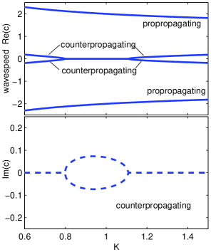
Figure 2: The dispersion relationship (39) for the case where $c_{g1}=c_{g2}$ with $Ri=1$, i.e. (40). The top graph shows the real wavespeeds of the four modes as a function of $K$. The propropagating modes always remain stable while the two counter-propagating modes become unstable when they phase lock with each other and their phase speeds become zero. The bottom graph shows the imaginary wavespeeds of the counter-propagating modes.

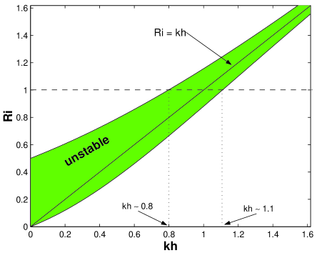
Figure 3: The incidence of linear instability (shaded region) for given values of the bulk-Richardson Number Ri and the wavenumber $k$. In this particular example $c_{{}_{g1}}=c_{{}_{g2}}$. Shown with a dashed horizontal line is the specific value of Ri $=1$ that is examined in the text. Instability occurs approximately for the range $0.80<kh<1.11$ (shown with dotted lines). The range of instability shrinks as $kh\gg 1$ and stradles the line Ri $=kh$ (also depicted).

We ask the question: for the unstable mode in isolation, what are the relative amplitudes and phases of the four kernel waves with respect to each other? Let us say define the vector $\mathbf{V}=(\tilde{\zeta}_{{}_{1+}},\tilde{\zeta}_{{}_{1-}},\tilde{\zeta}_{{}_{2+}},\tilde{\zeta}_{{}_{2-}})^{\mathrm{T}}$, then we see that (38) can be rewritten as

$$c\mathbf{V}=\mathbb{L}\mathbf{V}$$ (43)

in which $\beta\equiv{c_{g}}e^{-2K}/2$ and

$$\mathbb{L}\equiv\left(\begin{array}[]{cccc}c_{g}+U&0&\beta&-\beta\\ 0&-c_{g}+U&\beta&-\beta\\ \beta&-\beta&c_{g}-U&0\\ \beta&-\beta&0&-c_{g}-U\end{array}\right).$$ (44)

In the diagonal basis (denoted by primes) this system may be rewritten as

$$c\mathbf{V}^{\prime}=\mathbb{C}\mathbf{V}^{\prime},\qquad\mathbb{C}\equiv diag(+c_{{}_{-}},-c_{{}_{-}},+c_{{}_{+}},-c_{{}_{+}}).$$ (45)

where $\mathbf{V}^{\prime}=\mathbb{R}\mathbf{V}$ for the rotation vector $\mathbb{R}$. The columns of the inverse rotation matrix $\mathbb{R}^{-1}$ are composed of the eigenvectors of $\mathbb{L}$ (respecting the order of the eigenvalues appearing in $\mathbb{C}$). We have written the matrix $\mathbb{C}$ so that the first position represents the mode that can go unstable. Thus, if we wish to observe this mode in isolation we must require the following three equations

$$\mathbb{R}_{2n}\mathbf{V}_{n}=0,\qquad\mathbb{R}_{3n}\mathbf{V}_{n}=0,\qquad\mathbb{R}_{4n}\mathbf{V}_{n}=0,$$ (46)

($n=1,2,3,4$) be simultaneously satisfied. (Note that this is a generalization of the wave-mode isolation procedure we performed in Section III to follow the single kernel wave $\tilde{\zeta}_{+}$.) Since these are three equations with four unknowns, we ask what are the relative amplitudes and phases of the remaining three kernel waves when one has been set fixed to $1$. In this particular case of the unstable mode, we find that the relative behavior is most transparently appreciated when we gauge the action of the kernel waves with respect to the kernel wave $\tilde{\zeta}_{{}_{1-}}$ - i.e. the mode which, in the limit of large separation, corresponds to the wave propagating against the mean flow at the upper interface, cf. (38c) with $kh\gg 1$. By choosing $\tilde{\zeta}_{{}_{1-}}=1$ we can solve (46) for the remaining waves. Although $\mathbb{R}^{-1}$ may be written down analytically the solution for $\mathbb{R}$ is quite cumbersome and, as such, we depict a typical example numerically of the resulting behavior in Fig. 4. To be specific, we write each kernel wave in terms of its amplitude and phase, i.e.

$$\tilde{\zeta}_{{}_{1\pm}}=A_{{}_{1\pm}}e^{i\epsilon_{{}_{1\pm}}},\qquad\tilde{\zeta}_{{}_{2\pm}}=A_{{}_{2\pm}}e^{i\epsilon_{{}_{2\pm}}}.$$

By construction $A_{{}_{1-}}=1,\ \epsilon_{{}_{1-}}=0$. In the figure we plot the relative amplitudes and phases for the remaining waves with respect to $\tilde{\zeta}_{{}_{1-}}$ as one sweeps through wavenumber $K$.

We first note that in the limit of large wavenumber $\beta$ becomes negligible and the four equations of (43) decouple. This means to say that the four kernel modes propagate not “knowing” of the other waves or interfaces. This trend is represented in Fig.4 for $kh\gg 1$ - which shows the amplitudes of the remaining modes (i.e. $\tilde{\zeta}_{{}_{1+}},\tilde{\zeta}_{{}_{2\pm}}$) to go to zero as well. In the unstable zone (roughly $0.8<K<1.2$) the amplitudes of $\tilde{\zeta}_{{}_{1-}}$ and $\tilde{\zeta}_{{}_{2+}}$ stay equal, i.e. $A_{{}_{1-}}=A_{{}_{2+}}=1$, and the same goes for the the other two modes $A_{{}_{1+}}=A_{{}_{2-}}$ although they do not remain constant in the instability range as do the other pair. For this particular set of parameters the amplitudes of $A_{{}_{1+}},A_{{}_{2-}}$ are quite small compared to $A_{{}_{1-}}$ and this feature can aid us in developing a mechanical rationalization of the instability (see next section). We note that the phases also show an eastward tilt with respect to each other in the unstable regime: $\epsilon_{{}_{2+}}$ begins to show a positive phase with respect to $\epsilon_{{}_{1-}}=0$ as well as $\epsilon_{{}_{1+}}$ showing a positive phase with respect to $\epsilon_{{}_{2-}}=-\pi$ (the latter, incidentally, stays fixed throughout).

Due to the symmetries of the normal modes we note that the action and relative configuration of the kernel waves for the stable mode (i.e. $-c_{{}_{-}}$) is also represented in the figure with two modifications: the first of these is to set $c_{{}_{-}}\rightarrow-c_{{}_{-}}$ while the second would be to interchange the roles between $\tilde{\zeta}_{{}_{1-}}$ and $\tilde{\zeta}_{{}_{2+}}$ and between $\tilde{\zeta}_{{}_{2-}}$ and $\tilde{\zeta}_{{}_{1+}}$. In the exponentially decaying regime $\tilde{\zeta}_{{}_{2+}}$ starts to show a westward drift of its phase with respect to $\tilde{\zeta}_{{}_{1-}}$.

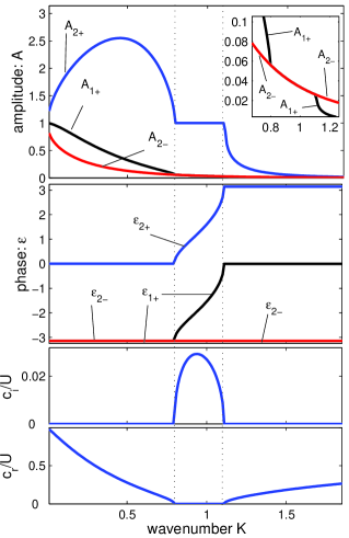
Figure 4: Phase and amplitude diagram for the unstable mode ($+c_{{}_{-}}$) in which $Ri=1$. All kernel wave phases and amplitudes are measured against the wave $\tilde{\zeta}_{{}_{1-}}$ which is set with $A_{{}_{1-}}=1,\epsilon_{{}_{1-}}=0$. The panels on the right shows the complex wave speeds for the unstable mode ($+c_{{}_{-}}$) as a function of $K$. The band of instability in $K$ is delineated with dotted lines. For $K\gg 1$ all mode amplitudes go to zero leaving behind only the wave $\tilde{\zeta}_{{}_{1-}}$. In the unstable regime $\zeta_{{}_{2+}}$ shares the same amplitude as $\tilde{\zeta}_{{}_{1-}}$ but begins to show an eastward tilt (in the same sense of the shear) of its phase, $\epsilon_{{}_{2+}}>0$ as one sweeps thru $K$. In the unstable phase, the amplitudes of the other two modes (i.e. $\tilde{\zeta}_{{}_{1+}},\tilde{\zeta}_{{}_{2-}}$) also lock together and there is also an eastward tilt of their phases with respect to each other in this range (i.e. of $\epsilon_{{}_{1+}}$ with respect to $\epsilon_{{}_{2-}}$). Note that the amplitudes of $A_{{}_{2}-}$ and $A_{{}_{1+}}$ in this regime are small compared to the other two amplitudes. The circles represent the function $\beta\sin(\epsilon_{{}_{2+}}-\epsilon_{{}_{1-}})$.

IV.2 Formulation as an initial value problem

The equations describing the general linearized response also offers insights which will aid us in rationalizing the instability uncovered here. Thus we consider the general temporal response of the equations of motion (37) by adopting the strategy of Heifetz & Methven (2005)heifetzCRW and inserting into those equations the assumed forms

$$\tilde{\zeta}_{{}_{1+}}=Z_{{}_{1+}}(t)e^{i\varepsilon_{{}_{1+}}(t)},\quad\tilde{\zeta}_{{}_{1-}}=Z_{{}_{1-}}(t)e^{i\varepsilon_{{}_{1-}}(t)},$$

$$\tilde{\zeta}_{{}_{2+}}=Z_{{}_{2+}}(t)e^{i\varepsilon_{{}_{2+}}(t)},\quad\tilde{\zeta}_{{}_{2-}}=Z_{{}_{2-}}(t)e^{i\varepsilon_{{}_{2-}}(t)}.$$ (47)

After equating real and imaginary parts we have the eight ode’s: four for the amplitudes,

$$\dot{Z}_{{}_{1+}} = k\beta\left[Z_{{}_{2+}}\sin\bigl{(}\varepsilon_{{}_{2+}}-\varepsilon_{{}_{1+}}\bigr{)}-Z_{{}_{2-}}\sin\bigl{(}\varepsilon_{{}_{2-}}-\varepsilon_{{}_{1+}}\bigr{)}\right],$$ (48a)

$$\dot{Z}_{{}_{1-}} = k\beta\left[Z_{{}_{2+}}\sin\bigl{(}\varepsilon_{{}_{2+}}-\varepsilon_{{}_{1-}}\bigr{)}-Z_{{}_{2-}}\sin\bigl{(}\varepsilon_{{}_{2-}}-\varepsilon_{{}_{1-}}\bigr{)}\right],$$ (48b)

$$\dot{Z}_{{}_{2+}} = k\beta\left[-Z_{{}_{1+}}\sin\bigl{(}\varepsilon_{{}_{2+}}-\varepsilon_{{}_{1+}}\bigr{)}+Z_{{}_{1-}}\sin\bigl{(}\varepsilon_{{}_{2+}}-\varepsilon_{{}_{1-}}\bigr{)}\right],$$ (48c)

$$\dot{Z}_{{}_{2-}} = k\beta\left[-Z_{{}_{1+}}\sin\bigl{(}\varepsilon_{{}_{2-}}-\varepsilon_{{}_{1+}}\bigr{)}+Z_{{}_{1-}}\sin\bigl{(}\varepsilon_{{}_{2-}}-\varepsilon_{{}_{1-}}\bigr{)}\right],$$ (48d)

and four for the respective phases,

$$\dot{\varepsilon}_{{}_{1+}}=-k(U+c_{g})$$

$$-k\beta\left[\frac{Z_{{}_{2+}}}{Z_{{}_{1+}}}\cos\bigl{(}\varepsilon_{{}_{2+}}-\varepsilon_{{}_{1+}}\bigr{)}-\frac{Z_{{}_{2-}}}{Z_{{}_{1+}}}\cos\bigl{(}\varepsilon_{{}_{2-}}-\varepsilon_{{}_{1+}}\bigr{)}\right],\ \ \ \ \ \ \$$ (48e)

$$\dot{\varepsilon}_{{}_{1-}}=-k(U-c_{g})$$

$$-k\beta\left[\frac{Z_{{}_{2+}}}{Z_{{}_{1-}}}\cos\bigl{(}\varepsilon_{{}_{2+}}-\varepsilon_{{}_{1-}}\bigr{)}-\frac{Z_{{}_{2-}}}{Z_{{}_{1-}}}\cos\bigl{(}\varepsilon_{{}_{2-}}-\varepsilon_{{}_{1-}}\bigr{)}\right],$$ (48f)

$$\dot{\varepsilon}_{{}_{2+}}=-k(-U+c_{g})$$

$$-k\beta\left[\frac{Z_{{}_{1+}}}{Z_{{}_{2+}}}\cos\bigl{(}\varepsilon_{{}_{2+}}-\varepsilon_{{}_{1+}}\bigr{)}-\frac{Z_{{}_{1-}}}{Z_{{}_{2+}}}\cos\bigl{(}\varepsilon_{{}_{2+}}-\varepsilon_{{}_{1-}}\bigr{)}\right],$$ (48g)

$$\dot{\varepsilon}_{{}_{2-}}=-k(-U-c_{g})$$

$$-k\beta\left[\frac{Z_{{}_{1+}}}{Z_{{}_{2-}}}\cos\bigl{(}\varepsilon_{{}_{2-}}-\varepsilon_{{}_{1+}}\bigr{)}-\frac{Z_{{}_{1-}}}{Z_{{}_{2-}}}\cos\bigl{(}\varepsilon_{{}_{2-}}-\varepsilon_{{}_{1-}}\bigr{)}\right].$$ (48h)

From the analysis of the previous section, an unstable normal mode implies a number of relationships to stand between the quantities appearing in (48): that (i) that $\dot{\varepsilon}_{{}_{1\pm}}=0,\dot{\varepsilon}_{{}_{2\pm}}=0$ since the modes do not “propagate” but are standing in that instance, (ii) $\varepsilon_{{}_{2+}}=\pi+\varepsilon_{{}_{1+}}$, and $\varepsilon_{{}_{1-}}=\pi+\varepsilon_{{}_{2-}}$, (iii) $Z_{{}_{2+}}=Z_{{}_{1-}}$ and $Z_{{}_{1+}}=Z_{{}_{2-}}$. If we assign to $\sigma$ the meaning of a growth rate then it is related to the phase differences according to

$$\sigma=k\beta\sin\Bigl{(}\varepsilon_{{}_{2+}}-\varepsilon_{{}_{1-}}\Bigr{)},$$

in Figure 1 we have depicted $\sigma$ - in terms of Im($c$) which is equal to $-\sigma/ik$.

In the extreme limit where $\beta\ll 1$, together with the above stated relationships, we may establish the relative scaling behavior between $Z_{{}_{1-}}$ and $Z_{{}_{1+}}$ and between $Z_{{}_{2+}}$ and $Z_{{}_{2-}}$ in the unstable normal mode regime. Taking for instance (48e), if one is in the instability range then it immediately follows that

$$Z_{{}_{1+}}=\beta\frac{Z_{{}_{1-}}}{U+c_{g}}+{\cal O}\left({\beta^{2}}\right),$$ (49)

where we have exploited the fact that $Z_{{}_{2+}}=Z_{{}_{1-}}$. The scaling on $Z_{{}_{2-}}$ immediately follows from the equality of it to $Z_{{}_{1+}}$. We learn from this analysis an important clue: namely that in the limit where $\beta\ll 1$ the main actors involved in the development of the normal-mode instability are the kernel waves $\zeta_{{}_{2+}}$ and $\zeta_{{}_{1-}}$ while the other two kernel waves, $\zeta_{{}_{2-}}$ and $\zeta_{{}_{1+}}$, should be viewed as being slaved (in a qualitative sense) to the former two. This fact allows us to interpret the instability with greater transparency. We devote our attention to this in the next section.

IV.3 The normalmode instability rationalized

Although for this problem there are four KGW waves, the general normal-mode analysis indicates that exponential behavior is mainly rooted in the two individual KGWs which move against the prevailing (background) flow. Take for example the KGW propagating against the flow associated with the top interface: if one were to move into the rest frame at that level, i.e. in a frame moving eastward with velocity $U$, then this wave would appear to move westward. By symmetry reasons the corresponding KGW on the bottom interface would appear to move eastward. Thus to an observer in the laboratory frame the culprit KGWs propagate with a speed which is slower than the local flow. As mentioned earlier, we shall refer to these waves with this character as counterpropagating-KGWs. Taken as individual waves, i.e. free of cross-layer interactions, the counterpopagating KGWs are those KGWs whose wavespeeds are $\pm(U-c_{g})$. Those KGWs that propagate with the local flow, i.e. those which have wavespeeds equal to $\pm(U+c_{g})$, will be referred to as propropagating-KGWs.

We further remind ourselves that when layers interact, the primary (eigen)modes leading to instability come in pairs - showing either an eastward or westward propagation of the eigenmode pattern. In general the individual eigenmodes are structures composed of all four KGWs however we see from the arguments in the last section that when $\beta$ is small, the eigenmodes are primarily constructed of only the two counter-propagating-KGWs $\zeta_{{}_{1-}}$ and $\zeta_{{}_{2+}}$ while the propropagating-KGWs, namely $\zeta_{{}_{1+}}$ and $\zeta_{{}_{2-}}$ are (in a sense) slaved to the former two. Instability develops by which the modes in question show wavespeeds passing through zero. Thus at marginality we have two wave patterns that both appear standing to the observer in the laboratory frame.

From these observations we shall argue here that the mechanism for instability in this problem is strongly analogous to the process leading to the instability of CRWs as in Rayleigh’s classic problem. Thus we propose that the dynamics are governed only by the action of the counter-propagating-KGWs for $\beta\ll 1$ (i.e. $K\gg 1$). Since in that case the propropagating-KGWs are slaved to the counter-propagating ones, we posit that the dynamical evolution of this system (for $c_{g1}=c_{g2}=c_{g}$) is given by the more simpler form

$$\left(\frac{\partial}{\partial t}+ik\tilde{c}\right)\tilde{\zeta}_{{}_{1-}} = -ik\beta\tilde{\zeta}_{{}_{2+}},$$ (50)

$$\left(\frac{\partial}{\partial t}-ik\tilde{c}\right)\tilde{\zeta}_{{}_{2+}} = ik\beta\tilde{\zeta}_{{}_{1-}},$$ (51)

where $\tilde{c}\equiv U-c_{g}$. We note immediately that mathematically speaking, (50-51) have the same structure as the equations describing the evolution of interacting kernel Rossby waves (KRWs, cf. 9a-c of Heifetz & Methven, 2005 heifetzCRW ). It means to say that these mutual interaction of KGW waves (in this limit) may be considered and rationalized in the same manner in which interacting KRWs are rationalized. The familiar instability properties exhibited in the problem of CRWs follows onto the quality of these dynamics as well, in particular, the co-action of hindering-helping of individual waves when instability is present.

We may further rationalize this instability, as viewed through through the lens of the reduced model (50-51), in terms of the stability criterion of Hayashi & Young (1987) and Sakai (1989) hayashi_young ; sakai referred to in the Introduction. Inspection of the dispersion relationship for the system (50-51), e.g. the counter-propagating modes in Fig. 2, shows that the those modes which become unstable propagate opposite to each other for wavenumbers just beyond the onset of instability. Their Doppler-shifted frequencies at onset (i.e. when $c=0$ for both waves) are $\pm k\tilde{c}$ respectively and they are almost equal by virtue of $\tilde{c}$ being almost zero in the limit appropriate for this reduced model. And finally without the term $\beta$, which represents the mutual interaction of these waves, there is no chance for instability to occur.

V Normal modes of a foamy layer

We consider further results assuming the two density jumps represent the configuration of a foamy layer as discussed in the Introduction. In particular we will examine the atmosphere with stratification considered in Shtemler et al. (2007).Miki_2007 In other words we shall analyze an atmosphere in which the density of the air $\rho_{a}$ is $\delta$ times the density of the foam $\rho_{f}$ which is, in turn, $\delta$ times the density of the sea layer $\rho_{s}$. In terms of the density formulation given in (23) we make the following replacements $\rho_{0}\rightarrow\rho_{f}$ and

$$\Delta\rho_{1}\rightarrow\rho_{f}\frac{1-\delta}{\delta},\qquad\Delta\rho_{2}\rightarrow-\rho_{f}(1-\delta),$$

and for the velocities we have

$$c_{g1}^{2}\rightarrow\frac{c_{f}^{2}}{\delta},\qquad c_{g2}^{2}\rightarrow c_{f}^{2},\qquad c_{f}^{2}=\frac{g(1-\delta)}{2k},$$

where $0<\delta<1$. Considerations of this system in a small vicinity near $\delta=1$ recovers the dynamical behavior of the case studied in the previous section. The dispersion relationship (39) now appears as

$$\left(\frac{c}{U}\right)^{4}-\left(2+{\cal C}_{f}^{2}\frac{1+\delta}{\delta}\right)\left(\frac{c}{U}\right)^{2}-2{\cal C}_{f}^{2}\frac{1-\delta}{\delta}\left(\frac{c}{U}\right)+$$

$$\ \ \ \ \ \ 1-{\cal C}_{f}^{2}\frac{1+\delta}{\delta}+\frac{{\cal C}_{f}^{4}}{\delta}(1-e^{-4K})=0.$$ (52)

where ${\cal C}_{f}\equiv c_{f}/U$. Inspection of the above relationship suggests that when instability occurs, the unstable waves will have some propagation associated with them unlike the stratification considered in the previous section. In a similar fashion we define the quantity $R_{f}$ such that ${\cal C}_{f}^{2}\equiv R_{f}/K$ and where

$$\frac{1}{F_{r}}=R_{f}\equiv\frac{gh(1-\delta)}{2U^{2}},$$

which is related to the inverse of the Froude number. We show in Fig 5 the general trends for these circumstances when $R_{f}=1$. A non-zero value of $\delta$ means that when instability sets in, it is no longer stationary as in the previous section, but the modes in question are now propagatory. In the range of unstable wavenumbers the propagation speed is is also a function of $K$. For $R_{f}$ held fixed, as $\delta$ approaches zero the range of unstable wavenumbers gets smaller, the location of the unstable band shifts to larger wavenumbers and the peak growth rate in this unstable band similarly get smaller.

In Fig. 6 we display the results of fixing $\delta$ and varying the bulk Richardson number $R_{f}$. This time, however, we use numbers that figure to be relevant to the problem of hurricanes. Because the density ratio between water and air is one thousand to one we assume that $\delta=\sqrt{0.001}\approx 0.03$. Following Shtemler et al. (2007)Miki_2007 we take (as a rough order of magnitude estimate) for the foam layer thickness the figure $h=1$m. Because, empirically speaking, strong winds over water follow a logarithmic profile Powell et al. (2003) powell generate fits of this form to the data accumulated during hurricane over-flight missions. For hurricane force winds (i.e. winds exceeding 34 m$\cdot$s^-1 at 1km above the sea surface) the wind speed at 1m above the sea surface is approximately 20 m$\cdot$s^-1 as inferred from Figure 2 of Powell et al. (2003)powell . Thus we assume this figure for $U$. Roughly speaking, it means that the bulk Richardson number for these conditions is $R_{f}\sim 0.01$. The results depicted in Fig. 6 are for three values of $R_{f}=0.04,0.01,0.0024$. The trends appearing are that the peak growth rate increases as $R_{f}$ is made smaller although the unstable range in $K$ begins to narrow as well. Just as in the results of the previous section (e.g. see Fig. 3) there exists a critical value of $R_{f}(\delta)$ below which $K=0$ is also unstable. In general this is probably a pathology of the theory and one ought not to take too seriously the results at $K=0$. However, once $R_{f}$ dips below this value the range of unstable wavenumbers narrows. We note finally that the first wavenumber to be unstable at $R_{f}=0.01$ occurs at $K\approx 0.15$. We shall make a remark about this and its relationship to hurricane data in the next section.

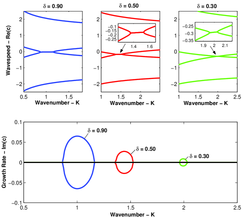
Figure 5: Wavespeeds and growth rates as a function of wavenumber $K$ for various values of $\delta$ at $Ri=1$. The top row of panels demonstrates the wavespeeds. Whenever instability sets in the wavespeeds of two modes merge. Unlike $\delta\approx 1$ theory, the wavespeeds are non-zero and have $K$ dependence when instability sets in. The bottom panel shows how the growth rate behaves as $\delta$ becomes small: (i) the range in $K$ for which growth occurs narrows and, (ii) and the amplitude of the maximum growth rate reduces.

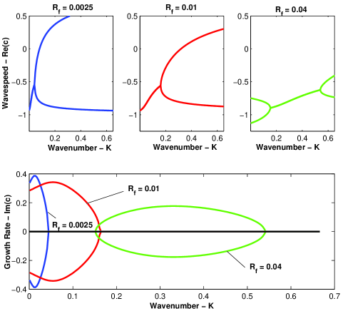
Figure 6: Wavespeeds and growth rates for a foamy layer as a function of wavenumber $K$ for various values of $R_{f}$ at $\delta=0.03$. The top row of panels demonstrates the wavespeeds of those modes demonstrating growth and decay only. The peak growth rates get larger for smaller values of the bulk Richardson number.

VI Summary and Discussion

VI.1 Recapitulation

We have studied how KGWs interact across two layers in a medium with globally constant shear. KGWs, along with KRWs heifetzCRW , are dynamical phenomena forming a subclass of KRGWs developed in Harnik et al. (2007)HHUL07 . In terms of the formalism developed, we have found that the interaction of KGWs under these conditions bear significant similarity to KRWs especially when instability sets in. For KGWs, the presence of a jump in the background density at some layer means that these places support the creation of vorticity which ultimately relates to the interpretation that such configurations are sources of baroclinic torques UH_07. Unlike KRWs, where a jump in the background shear produces a single propagating Rossby edge-wave, an isolated jump in density creates two surface gravity waves propagating with equal and opposite directions. These cohabitating (in the sense that they exist on the same layer) counter-propagating gravity waves can be cast into a a set of new variables which explicitly shows that the wave pair do not interact.

The KGW kernel is composed of the measure of the edge-wave vorticity and the amount which the surface has been displaced from equilibrium. Viewed in terms of this combination of physical variables, we have demonstrated how a single wave mechanically operates as it propagates. The vorticity field corresponds to a velocity field around the disturbed surface while the disturbed surface indicates how further vorticity is to be generated ahead of the peak of the wave. The disturbed surface creates this vorticity (in the sense of the mechanical description we present) because it looks like a displaced lever arm - when let free such a lever arm has the tendency to rotate about its equilibrium point and generate vorticity as a consequence. The true wave executes these steps continuously in a fluid way.

The analysis of the interaction of KGWs on two layers was facilitated here by assuming the density jumps to be the same across each layer which results in a normal mode problem that is analytically tractable. Because of the shear profile, the top layer moves with speed $U$ while the bottom layer moves with speed $-U$. In this case one has four normal modes (a co-habitating pair on each layer). Normal mode instability arises primarily through the interaction of two modes from each layer - these modes are ones which, in the absence of mutual interaction, would propagate against the background flow of the layer. The remaining two modes contribute less and less to the development of the instability when the layer separation (or, equivalently, the horizontal wavenumber) gets large. In this large separation limit, the resulting effective equations have the same mathematical form as the ones describing the (exact) development of unstable CRWs heifetz99 . This means to say that the mechanism behind this instability is qualitatively similar to the way instability emerges in the problem of CRWs.

VI.2 As being a CRW analog

In a sense the instability is the analog of the CRW instability and it is for this reason why we refer to this mode interaction process as the instability of counter-propagating gravity waves. Indeed the KGW may be interpreted as a (delta-function) vortex structure which propagates at some speed on the layer in question. Whereas in KRWs the source of the vorticity is the jump in the background vorticity, in KGWs the source is the baroclinicity that arises when the jump layer is perturbed. The ensuing dynamics are qualitatively similar in all other major respects. It is also true that both left and right going waves become excited on a layer when a single KGW propagates along the other. In this way the conception and rationalization of the dynamics of four KGWs is more complicated. But, and we reiterate this point, the basic qualitative features of the instability involves the dynamical influence between only two of the KGWs, namely those that counterpropagate with respect to the background flow at their respective interfaces, and the processes at work resemble the mechanism responsible for the instability of CRWs.

VI.3 The normal-mode instability, its rationalization and relationship to the Miles-Howard Theorem

As the disturbances considered here preclude the possibility of an inflexion point instability (i.e. the Rayleigh criterion), the character of disturbances falls under the purview of the Miles-Howard theorem. The Miles-Howard theorem miles61 ; howard61 for the stability of plane-parallel stratified shear flows states that a sufficient criterion for stability of normal-mode disturbances is that the Richardson number (J) of the flow be everywhere greater than $\frac{1}{4}$ in the domain. That is to say that a necessary condition for instability is that somewhere in the flow

$${\rm J}\equiv-\frac{g}{\rho}{\frac{d\rho}{dz}}\cdot\frac{1}{(dU/dz)^{2}}<\frac{1}{4},$$ (53)

where the quantities defining J are in dimensional units. Because this is a plane-Couette flow $dU/dz$ is everywhere defined and not equal to zero. For the “stably” stratified fluid we have considered here, i.e. $-(g/\rho)d\rho/dz>0$, J would then be described by two delta-functions, with positive coefficients, centered on the locations of the density discontinuity. This means to say that J is zero everywhere except at the points where the density discontinuity occurs. At the very least, the instability uncovered here satisfies the necessary Miles-Howard criterion for normal-mode instability as J is less than $\frac{1}{4}$ in substantial parts of the flow.

What is interesting to reflect upon is that this instability might be the simplest kind possible in a shear flow absent vorticity waves. Regular (inviscid) plane-Couette flow, though satisfying the necessary condition for instability, is however stable as is a plane-Couette flow with a single density interface. All that is needed for a plane-Couette profile to exhibit normal-mode instability is for there to exist a second density interface.

Given the previous discussion it seems to us that normal-mode instability in shear flows merely requires the presence of counter-propagating waves of any sort. Indeed a cursory review of some previous work reveals: (i) the classic instability emerging from the model problem investigated by RayleighRayleigh1880 has been reinterpreted as arising out of the interaction of phase-locked counter-propagating vorticity waves bretherton ; heifetz99 (i.e. Rossby edge waves), (ii) a simplified restricted version of Holmboe’s instability holmboe62 has been shown to be emerging out of the interaction of a pair of counter-propagating waves in which one is a vorticity wave and the other is a gravity waveBM94 and, (iii) here we have demonstrated yet another instability borne out of the interaction of counter-propagating waves which are comprised, in this instance, of phase-locked gravity waves.

This leads to the apparently counterintuitive conclusion that a convectively stable stratification can destabilize a flow profile that is stable in the unstratified case. It is nevertheless important to recall here that this result is not in contradiction with conventional linear stability criteria. Indeed, in the presence of stratification, one of these criteria is the Miles-Howard criterion found in (53) which places no limitations on the wind curvature. It means that there is a much larger array of wind profiles that can be unstable in the stratified case than in the unstratified one.

VI.4 Foamy layers and a conjecture

We observe that the range of unstable wavenumbers is finite in the case where the density jumps are the same (Section IV). But, in comparison, both the wavenumber range and the maximum growth rate of the instability when considered in a foamy layer (Section V) reduces as the the density parameter describing the foam $\delta$ gets small. However consideration of parameters having more relevance to real atmospheric phenomenon reveals some interesting predictions. When numbers appropriate for observed hurricanes are utilyzedpowell ; Miki_2007 we find that they correspond to bulk Richardson numbers ($R_{f}$) in the vicinity of $0.01$. Inspection of the growth rates show that the wavenumber for the onset of instability is $kh\approx 0.15$ in which $h$ is the nominal height of the foam layer. Assuming, as we have, that $h=1$m it means that the wavelength of this unstable mode is approximately $\lambda\sim 45$m. An inspection of Figure 4a in Powell et al. (2003)powell shows a photograph of the sea from a quarter kilometer height during a hurricane whose windspeeds, as measured at the height of the aircraft, are approximately $45$ m$\cdot$s^-1. The image shows the foamy patches and the length scales of the groupings that appear is approximately $30$m in length. Figure 4b of the same work shows the foamy patches after the windspeeds have increased to $55$ m$\cdot$s^-1 and one sees clearly that the foam patches have covered the entirety of the sea surface. Since larger values of the windspeed correspond to smaller values of critical wavenumbers, the theory developed here shows at least the same trend in the observed photographs.

Of course there are obvious shortcomings of applying the theory developed here to the circumstances noted for this hurricane observation: (i), that the height of the foam layer was assumed since there are no direct observations to that end from the data available, (ii) it is not at all clear if there exists a “laminar” foam layer from which a secondary instability develops creating the frothy foam layer observed in these photographs and, (iii) the assumption of a linear velocity profile in place of a logarithmic one is clearly a gross simplification. The latter assumption is probably satisfactory on the scale of the foam layer but certainly breaks down if one tries to extend it much beyond a logarithmic scale height of the layer thickness (e.g. $10$m or higher if $h=1$m). Thus although the apparent consistency observed between this simple theory and the observations made is not proof that the theory developed here is relevant to such complicated processes (i.e. hurricane-sea interfaces), it is at least encouraging that this theory makes predictions which are of at least the same order of magnitude as the structures observed. As such we treat this discussion as being purely conjecture at this stage.

Appendix A Derivation

We show here the step-by-step derivation that ultimately leads to the equation set (26-29). The basic density profile and its derivatives, written in terms of $b$, is itemized here,

$$\frac{d\bar{b}}{dz}=\frac{g\Delta\bar{\rho}_{1}}{\rho_{0}}\delta(z-z_{1})+\frac{g\Delta\bar{\rho}_{2}}{\rho_{0}}\delta(z-z_{2}),$$ (54)

$$\frac{\partial b}{\partial x}=-\frac{g\Delta\bar{\rho}_{1}}{\rho_{0}}\frac{\partial\zeta_{1}}{\partial x}\delta(z-z_{1})-\frac{g\Delta\bar{\rho}_{2}}{\rho_{0}}\frac{\partial\zeta_{2}}{\partial x}\delta(z-z_{2}),\ \ \ \ \ ,$$ (55)

$$\left(\frac{\partial}{\partial t}+\bar{U}\partial_{x}\right)b=-\frac{g\Delta\bar{\rho}_{1}}{\rho_{0}}\delta(z-z_{1})\left(\frac{\partial}{\partial t}+\bar{U}\partial_{x}\right)\zeta_{1}$$

$$\ \ \ -\frac{g\Delta\bar{\rho}_{2}}{\rho_{0}}\delta(z-z_{2})\left(\frac{\partial}{\partial t}+\bar{U}\partial_{x}\right)\zeta_{2}.$$ (56)

these expressions are inserted into the governing equations (5-6),

$$\left(\frac{\partial}{\partial t}+\bar{U}\partial_{x}\right)q=(g/\rho_{0})\frac{\partial\zeta_{1}}{\partial x}\delta(z-z_{1})$$

$$\ \ \ \ \ \ \ \ \ \ \ \ \ +(g/\rho_{0})\frac{\partial\zeta_{2}}{\partial x}\delta(z-z_{2}),$$ (57)

$$\left(\frac{\partial}{\partial t}+\bar{U}\partial_{x}\right)\left[\frac{g\Delta\rho_{1}}{\rho_{0}}\zeta_{1}\delta(z-z_{1})+\frac{g\Delta\rho_{2}}{\rho_{0}}\zeta_{2}\delta(z-z_{2})\right]$$

$$\ \ \ \ \ \ \ \ =w\frac{g\Delta\rho_{1}}{\rho_{0}}\delta(z-z_{1})+w\frac{g\Delta\rho_{2}}{\rho_{0}}\delta(z-z_{2}).$$ (58)

From inspection above it is clear that the vorticity of the system takes on delta function character at all of the jumps of the system. This then means applying the ansatz

$$q=\hat{q}_{1}(x,t)\delta(z-z_{1})+\hat{q}_{2}(x,t)\delta(z-z_{2}).$$

Collecting all terms of like delta functions, one may set each of the coefficients to zero because of the mutual “orthogonality” of the delta functions. In a sense this system has been discretized. This results in the following,

$$\left(\frac{\partial}{\partial t}+U\frac{\partial}{\partial x}\right)\hat{q}_{1} = hN^{2}_{{}_{1}}\frac{\partial\zeta_{1}}{\partial x},$$ (59)

$$\left(\frac{\partial}{\partial t}+U\frac{\partial}{\partial x}\right)\zeta_{1} = w(h,x),$$ (60)

$$\left(\frac{\partial}{\partial t}-U\frac{\partial}{\partial x}\right)\hat{q}_{2} = hN^{2}_{{}_{2}}\frac{\partial\zeta_{2}}{\partial x},$$ (61)

$$\left(\frac{\partial}{\partial t}-U\frac{\partial}{\partial x}\right)\zeta_{2} = w(-h,x).$$ (62)

To recover (26-29) we apply the Fourier ansatz (25) to (59-62). With which it immediately follows that the streamfunction field $\psi$ (subject to the usual jump conditions) is the familiar form,

$$\psi=-\left(\frac{\tilde{q}_{1}}{2k}e^{-k|z-h|}+\frac{\tilde{q}_{2}}{2k}e^{-k|z+h|}\right)e^{ikx}+{\rm c.c.}.$$ (63)

References

- (1) F.P. Bretherton, “Baroclinic instability and the short wave cut-off in terms of potential vorticity,” Q. J. R. Meteorol. Soc. 92, 335 (1996).
- (2) E. Heifetz, C. H. Bishop & P. Alpert, “Counter-propapagating Rossby waves in the barotropic Rayleigh model of shear instability,” Q.J.R. Meterol. Soc. 125, 2835 (1999).
- (3) E. Heifetz & J. Methven, “Relating optimal growth to counterpropagating Rossby waves in shear instability,” Phys. Fluids 17, 064107 (2005).
- (4) Lindzen, R.S., “Instability of plane parallel shear-flow (toward a mechanistic picture of how it works,” Pure Appl Geophys., 126 103 (1988).
- (5) N. Harnik and E. Heifetz, “Relating over-reflection and wave geometry to the counter propagating Rossby wave perspective: toward a deeper meachnistic understanding of shear instability,” J. Atmos. Sci. 64, 2238, (2007).
- (6) N. Harnik, E. Heifetz, O. M. Umurhan & F. Lott, “A generalized wave kernel approach to plane parallel stratified shear flow,” J. Atmos. Sci. (To Appear) (2007).
- (7) Sakai, S., “Rossby-Kelvin instability: a new type of ageostrophic instability casused by a resonance between Rossby waves and gravity waves,” J. Fluid Mech. 202, 149, (1989).
- (8) Baines, P.G. & Mitsudera, H., “On the mechanism of shear flow instabilities,” J. Fluid Mech. 276, 327, (1994).
- (9) Caulfield, C-C. P., “Multiple linear instability of layered stratified shear flow,” J. Fluid Mech. 258, 255, (1994).
- (10) Holmboe, J., “On the behaviour of symmetric waves in stratified shear layers,” Geophys. Publik., 24, 67, (1962).
- (11) Hayashi, Y.-Y. & Young, W.R., “Stable and unstable shear modes of rotating parallel flows in shallow water,” J. Fluid Mech. 184, 477, (1987).
- (12) Lord Rayleigh, “On the stability, or instability, of certain fluid motions,” Proc. London Math. Soc. 9, 57 (1880).
- (13) Newell, A. & Zakharov, V.E., “Rough sea foam,” Phys. Rev. Lett. 69, 1149 (1992).
- (14) Powell, M.D., Vickery, P.J. & Reinhold, T.A., “Reduced drag coefficient for high wind speeds in tropical cyclones,” Narure 422, 279 (2003).
- (15) Shtemler, Y.M., Golbraikh, E. & Mond, M., “Wind instability of a foam layer sandwiched between the atmosphere and the ocean,” Submitted to Phys. Rev. Let., (2007).
- (16) Craik, A. & Adam, J.A., “ ’Explosive’ resonant wave interactions in a three-layer fluid flow,” J. Fluid Mech. 92, 15 (1979).
- (17) Schmid, P. J. & Henningson, D.S., Stability and Transition in Shear Flows, Springer, New York (2001).
- (18) Booker, J. R. & F. P. Bretherton, “The critical layer for internal gravity waves in a shear flow,” J. Fluid Mech. 27, 513 (1967).
- (19) Miles, J. W., “On the stability of heterogeneous shear flows,” J. Fluid Mech. 10, 496 (1961).
- (20) Howard, L. N. “Note on a paper of John W. Miles,” J. Fluid Mech. 10, 509 (1961).
- (21) Van Duin, C. A. & H. Kelder, “Reflection properties of internal gravity waves incident upon an hyperbolic tangent shear layer,” J. Fluid. Mech. 120, 505 (1982).